Affect Learning?
Moffat Mathews and Tanja Mitrovi´c Computer Science & Software Engineering,
University of Canterbury, New Zealand. (moffat,tanja)@cosc.canterbury.ac.nz
Abstract. We examined high-level help (HLH) seeking behaviour of students by data mining in SQL-Tutor. Students who used HLH very frequently had the lowest learning rate; their learning was also shal-low. They attempted very difficult problems compared to other groups but only solved very easy problems, suggesting that they were usually situated well beyond their Zone of Proximal Development. They also abandoned a large number of problems without solving them. Manual inspection of the logs showed erratic problem solving behaviour, sug-gesting a “guess and copy” strategy.
The group of students who used HLH very infrequently seemed to con-tain two distinct sub-groups: students with high expertise, and students with very low expertise who still did not use HLH. Learning rates were highest for students who used moderate HLH. Students with lower us-age of HLH solved the most difficult problems comparatively, without the use of HLH, and had high learning rates, suggesting the ITS is most beneficial for this group of students.
Key words: Help-seeking behaviour, data mining
1
Introduction
This paper presents the initial results of data mining student models and log files in SQL-Tutor [1]. The research conducted in this paper is the first in a series of steps towards a project designed to develop a general framework for adapting pedagogical strategies in Intelligent Tutoring Systems (ITSs). Part of the challenge of designing such a framework is to identify the various contexts in which students find themselves when working in an ITS, and understand their behaviour when confronted with such a context. As researchers and developers, we are also interested in the effects of this behaviour on learning. Research is continuing into various aspects of help seeking behaviour [2], including investi-gating the misuse of help and feedback in ITSs [3, 4]. In this step of the research, we explore one aspect of help-seeking behaviour in students: the frequency of high-level help (HLH) sought and its effect on learning.
Help in an ITS usually consists of tutor-specific help and domain-specific help. Tutor-specific help is help regarding the ITS itself. For example, this type
of help might show the student steps on how to submit a particular problem, or how to request a new problem. In contrast, domain-specific help concentrates on concepts within the domain irrespective of any tutoring system used.
Domain help can be categorised in many ways. One way is to class it into either dependent or concept-dependent help. Examples of problem-dependent help are hints or feedback messages provided for a particular problem or step within that problem. These can either be given before the problem is at-tempted (forward hints) or after a solution has been submitted (feedback). Con-cept dependent help is help on domain conCon-cepts and is usually given in the form of tutorials or feedback during a meta-cognitive dialogue (e.g. during reflection or self explanation).
Domain help can also be categorised into adaptive or non-adaptive help. Adaptive help is customised for the particular student, and is based on the student’s solution or their student model. An example of non-adaptive help is the full solution.
For this research, we have also categorised domain help into low-level help (LLH) and high-level help (HLH). Low and high level refer to the degree of help given. For example, showing the student a partial or full solution is classed as high-level help, whereas telling the student that they have made some errors is classed as low-level help. Sometimes, the process of giving higher degrees of help till the highest degree is reached is referred to as “bottoming out”. The highest degree of problem-dependent help is usually the full solution, either for the step or the entire problem. In this paper, we focus on the use of LLH and HLH to explore its effect on learning.
2
Problem-Dependent Help in SQL-Tutor
SQL-Tutor is an ITS designed to guide and support students in their deliber-ate practice in the domain of querying databases in Structured Query Language (SQL). SQL-Tutor has a long history of high learning rates and evaluation stud-ies, and is used in tertiary database courses as part of the curricula. Being a constraint-based modelling tutor, it stores domain knowledge as constraints (domain principles) and provides the student with multiple levels of domain-help depending on various factors, such as their current solution, their student model, and the constraints violated on this submission.
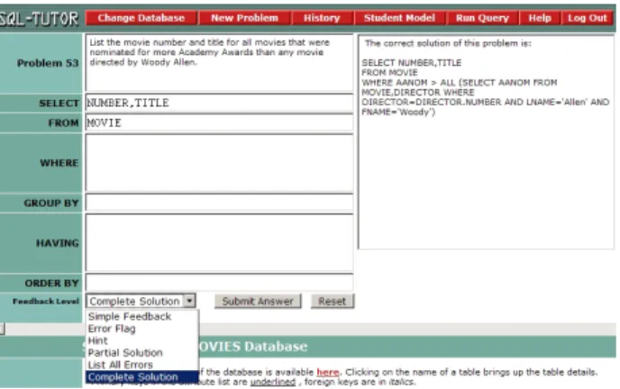
In SQL-Tutor, the problem-dependent, domain help is divided into six num-bered categories. These categories in order of degree of help are: 1. Simple feed-back, 2. Error flag, 3. Hint, 4. Partial solution, 5. List all errors, and 6. Full solution. The help level (also known as feedback level) is controlled on the inter-face by means of a simple combo box (see Fig. 1). At the start of a new problem, the tutor defaults to help level 1. On subsequent incorrect submissions, the tu-tor automatically increments the help level by one, to a maximum of 3 (i.e. hint). The student can override the help selection at any time by changing the value of the combo box. Help levels 4, 5, and 6 have to be specifically requested by the student. For this research, we have classed help levels 1-3 (inclusive) as
LLH, and help levels 4-6 (inclusive) as HLH. Furthermore, LLH is automatically incremented, but HLH is requested by the student.
Fig. 1. The SQL-Tutor task environment showing the combo box with the various levels of problem-dependent help. Here, the student has requested HLH (in this case, the full solution) for the problem, which is displayed in the feedback pane.
When a student reaches the task workspace (Fig. 1) in SQL-Tutor, they are presented with the problem in text format. More information regarding the context of the problem, such as information about the schema, is also presented with each problem. The solution workspace contains text areas in which students can work on their query. Once the student is content with their solution, they can submit it and receive feedback. The degree to which this feedback is given is dependent on the help level selected, as discussed above. It is this help - and more specifically, the difference between LLH and HLH used by students, that interests us for this paper.
3
Learning Curves
Learning curves are used to plot students’ learning over time. Learning a skill generally follows a power law, where the greatest improvement occurs early in the learning process. The formula for the power law is given in equation 1. More details about learning curves can be found in [5, 6].
E=χnα. (1)
Where: E is the error rate, χ is the performance on the first trial, n is the opportunity to practice the skill, andαis the learning rate.
Four main points are worth noting. First, the learning rate (α) shows the speed at which errors are reduced over the number of occurrences of a particular
skill or concept. The slope of the graph at various points depicts the learning rate at that point. Second,χ describes the students’ performance on the first trial, and therefore shows how difficult the students found the particular domain or problem set; the higher the number, the more difficult. Therefore, if the domain or problem set was kept similar and yet the χ values differed between groups of students, it could be argued that the group with the higher initial error rate (i.e. the group that performed better on the first trial and therefore found the domain easier than the other groups) must have had prior domain knowledge or higher expertise than the other groups. Third, the fit of the graph (R2) illustrates the variability of the data within that group. The fit shows how well students used the skill they learned previously i.e. transferability of the skill learned. The better the fit, the higher the transferability. And finally, learning curves gradually decrease in slope over time i.e. the learning rate reduces. The value of the bottom of the curve shows the probability of the student making an error in subsequent occurrences of the same concept i.e. how well the student has learned the concept. If the learning rate has decreased to near-zero, and the probability of making errors is still quite high (the bottom of the curve is high), then the student’s learning can be considered shallow. The lower the bottom of the curve, the deeper the learning.
4
The Data and the Methods Used
The main dataset (named dataset A) for this research was taken from an online version of SQL-Tutor that is available to students from around the world who were given free access when they bought certain SQL text books. Data for any student that made less than five attempts was excluded. The remaining data consisted of 1803 users who made a total of 100,781 attempts and spent just over 1,959 active hours on the system. Active hours is time spent actively solving the problem; not just session times. Students in this dataset on average solved 70% of the problems attempted; giving a grand combined total of 19,604 solved problems.
We extracted the number of submissions for each student from the individual student logs. Each submission was then categorised as either a valid attempt or a request for help (RFH).A valid attempt occurs whenever a student submits a solution that is different to their previous solution. An attempt need not be correct to be valid. When a student submits either an empty solution or the same solution twice in a row, this is interpreted as a RFH. Here, the student is hoping that more hints will be given on each submission. SQL-Tutor automatically increments the help level to a maximum of 3. Equation 2 shows the relationship between submissions, attempts, and RFH.
Submissions = Attempts + Requests for help (2) We further categorised each valid attempt into two categories: high-level help (HLH) attempts or low-level help (LLH) attempts, and deduced the total number of HLH attempts for each student. To normalise the HLH attempts value over all
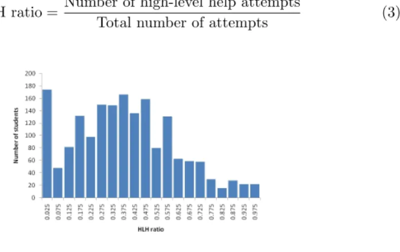
the students, we calculated an HLH ratio; 0≤HLH ≤1. (See equation 3). This ratio categorises students’ HLH seeking behaviour by showing us how frequently a student uses high-level help; low frequency HLH students are those that used high-level help very infrequently and vice versa. For example, a student with an HLH ratio of 1 uses HLH on every attempt, whereas a student with HLH ratio of 0.1 uses HLH once every ten attempts. Students were then ordered according to their HLH ratio; from low frequency HLH users to high frequency HLH users.
HLH ratio = Number of high-level help attempts
Total number of attempts (3)
Fig. 2.Frequency distribution of users in the various HLH user groups in dataset A.
A frequency graph of students and their HLH ratio is shown in Fig. 2. We then divided the population into ten groups (A1-A10) depending on their HLH ratio; the groups were 0.1 HLH apart. The logs and student models were analysed for each group, and learning curves were plotted.
Each problem in SQL-Tutor is assigned a difficulty level by the teacher. Dif-ficulty levels range from 1 (easiest) to 9 (most difficult). For each student, we mined the difficulty levels of problems attempted and recorded the maximum difficulty level of problem solved (MDLS). In our initial analysis, we used the MDLS to see how students from each group were able to learn skills and progress through to more difficult problems. Manual analysis of the logs showed that for students in the higher HLH groups, there was a large difference between the difficulty level of problems attempted and those solved; they attempted much more difficult problems than they solved. There also seemed to be a high num-ber of abandoned problems after valid attempts were made. Furthermore, in many cases the initial (incorrect) solutions were very different to the ideal so-lution. It was as though the high HLH students were employing a “guess then copy” method to solving problems. In contrast, the lower HLH students created answers that were usually more similar to a correct solution, then with each attempt submitted closer approximations to a correct solution until the problem was solved. Due to this, another metric, termed themaximum difficulty level of problem solved without using HLH (MDLS-WH) was also calculated and used.
The results are summarised in the next section.
Fig. 3.The learning curves for the ten HLH user groups (A1-A10).
5
Results and Discussion
5.1 Frequency Distribution of Users According to Their HLH
The frequency distribution graph in Fig. 2 shows the number of users grouped according to their HLH. This graph has an interesting shape. FromHLH >0.05, a positive skewed normal curve exists. There is also a peak external to the normal distribution in the first section of the graph: HLH ≤ 0.05; these are students that are very low users of HLH. Manual inspections of the logs seem to indicate the presence of at least two distinct types of students within this first section (HLH ≤ 0.05): one with higher domain expertise and the other with low domain expertise. This section of students needs to be analysed further. It is understandable that the students with high expertise are low users of HLH. However, the students with low expertise who do not use HLH could be those who either have low meta-cognitive (help-seeking) skills or, due to social norms, feel that looking at HLH constitutes a form of “cheating”. For comparison, frequency graphs were also plotted for two other smaller sets of data, and we found that the results were very similar. This shows that this trend is persistent across populations, and requires deeper analysis.
5.2 Learning Curves for Each HLH User Group
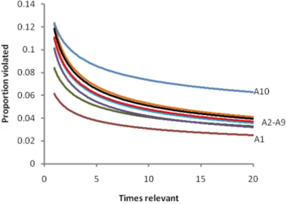
Learning curves were calculated and drawn for each of the ten groups (A1-A10). Fig. 3 shows the learning curves for all the groups plotted on the same graph for ease of comparison. To avoid clutter, the equations have been excluded from the graph but are listed in table 1.
Table 1.Power curve equations and fits (R2) for the ten HLH groups (A1-A10).
Group HLH ratio Power curve equationR2(Fit) A1 0.0 - 0.1 y= 0.061x−0.30 0.844 A2 0.1 - 0.2 y= 0.084x−0.31 0.956 A3 0.2 - 0.3 y= 0.101x−0.38 0.955 A4 0.3 - 0.4 y= 0.109x−0.37 0.956 A5 0.4 - 0.5 y= 0.110x−0.36 0.965 A6 0.5 - 0.6 y= 0.123x−0.39 0.961 A7 0.6 - 0.7 y= 0.122x−0.36 0.953 A8 0.7 - 0.8 y= 0.115x−0.35 0.953 A9 0.8 - 0.8 y= 0.118x−0.36 0.912 A10 0.9 - 1.0 y= 0.123x−0.22 0.956
1. The curves follow the same approximate order of the HLH use. The higher the HLH use, the shallower the learning. For example, students in the group A10 (those with the highest HLH) portray shallow learning; even when their learning rate approaches zero, their probability of making errors is still com-paratively high.
2. The fit for power curve is very high across all groups. The lowest fit for curve is in A1 (R2= 0.844). This could be because, as proposed earlier, A1 contains at least two distinct sub-groups of students: the students with high expertise, and the students with low expertise who persevere with problem solving without utilising HLH. The transferability of skills could vary within these sub-groups, reducing the overall fit.
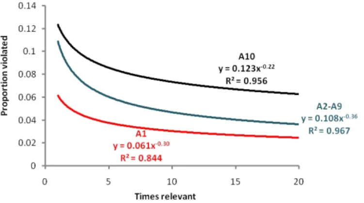
3. Since learning curves A2-A9 are very similar, this leaves us with three distinct categories of learning curves: A1, A2-A9, and A10. Fig. 4 shows the three learning curves plotted on a single graph. The middle range of HLH users displays similar learning (i.e. depth, learning rate, etc.), while the extreme high and low HLH users display markedly different learning.
4. The χ value increases as HLH use increases. This means that high HLH students find the domain more difficult than low HLH students. There is a marked difference between theχ value of A1 and the other groups. This could also show that A1 contains experts (or at least students with prior domain knowledge).
5. Curves A2-A9 report similarly high learning rates. A10, the highest HLH has the lowest learning rate (0.22). This could be because students that use HLH extremely frequently do not actively engage in the material, think for themselves, utilise their meta-cognitive skills (such as reflecting or explain-ing their actions), or participate in the benefits of deliberate practice (e.g. learning from errors). This causes much lower learning rates. The group of users that use HLH the least (i.e. group A1) has the second lowest learning rate. This could be because both the sub-groups (experts and low expertise students) in A1 both have low learning rates. The experts in A1 already find the domain easy, thus starting with low error rates (i.e.χis low), and there-fore reach their asymptote of learning very quickly. The novices in A1 who
persevere with problem solving without utilising HLH also have low learn-ing rates. In this case, the ITS is therefore most beneficial for the majority of students who are in the middle HLH range, producing relatively similar, high learning rates.
Fig. 4. The learning curves for the HLH user groups. In this graph (unlike Fig. 3), groups A2-A9 are combined. This was done as the curves for A2-A9 were very similar in nature.
5.3 Maximum Difficulty Level of Problems Solved by Students
The Zone of Proximal Development (ZPD) [7] is the area just beyond the stu-dent’s ability or more specifically, it is the difference between what a learner can do without help and what they cannot do without help. In ITS terms, the prob-lems found within the ZPD are just challenging enough for the student to solve with some help (i.e. LLH and moderate amounts of HLH) from the tutor. It is also said to be the area in which the highest rate of learning occurs. Like most ITSs, SQL-Tutor attempts to keep the student within their ZPD by guiding them through increasing levels of difficulty, while providing LLH, as their expertise in the domain increases; the student is also free to use HLH as necessary.
As mentioned earlier, problems in SQL-Tutor range in difficulty level from 1 to 9. Although the range (1-9) seems small, there is quite a difference in difficulty between levels, such that the difficulty (and type of concepts covered) between a problem of level 1 and another of level 5, for example, is considerable.
As discussed in the section above, we initially collected the maximum diffi-culty level of problems solved (MDLS); this included problems solved irrespective of the level of help used. Another metric,the maximum difficulty level of prob-lems solved without HLH (MDLS-WH) was also ascertained for each user from their logs. We determined that the MDLS-WH would give an indication of how far the user progressed through the domain on their own, and thus give us a
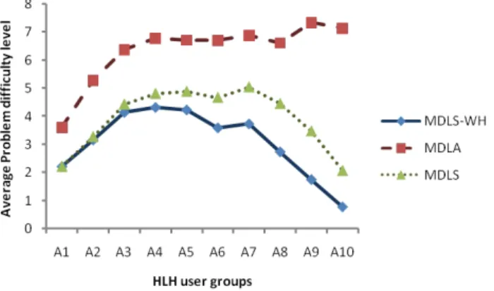
clue, albeit a vague one, of the student’s expertise in the domain. We also col-lected the maximum difficulty level of problems attempted (MDLA) for each student. The average MDLA, MDLS, and MDLS-WH for each HLH user group was calculated and plotted, and is shown in Fig. 5.
Fig. 5. The average maximum difficulty of problems attempted (MDLA), solved (MDLS), and solved without using HLH (MDLS-WH) for students in the HLH groups. Note the difference between the MDLA and MDLS-WH as HLH use increases.
As shown by the graph, the MDLA is always higher than the maximum difficulty of solved problems irrespective of any help levels. This is expected. The MDLS-WH increases steadily as HLH use increases, peaking at the A4 group (MDLS-WH = 4.32). After this, as HLH use increases, MDLS-WH decreases. The high HLH groups had very low MDLS-WH values (e.g. average MDL for A9 = 1.75) with the lowest MDLS-WH average occurring in the highest HLH user group (A10). Although the minimum problem difficulty level in SQL-Tutor is 1, the average MDLS-WH in A10 was 0.77. This was due to a number of students not solving any problems on their own, without HLH. The lowest HLH user group (A1) also reported a low MDLS-WH average (2.21). This is similar to the trend found in the learning curves above.
What is most interesting about this graph is the difference between the MDLA and MDLS-WH. The higher the HLH use, the greater the difference between the two graphs.
This shows that students who use low to moderate amounts of HLH, progress through the problem set, solving more difficult problems on their own compared to students who are either high or low frequency users of HLH. Students who are high HLH users attempt increasingly difficult problems, much harder problems on average than any other group of students. However, these students only solve very easy problems (either on their own, or using HLH), choosing to abandon problems after viewing the HLH. It is as if they have a very low expertise level, but choose to attempt problems far beyond their ZPD.
6
Future Work
Immediate future work for the authors include deeper analysis of certain groups more thoroughly (for example the composite group A1). In this paper, we divided the entire sample (evenly by HLH ratio) into ten groups. Another method would be to divide the sample into two separate groups first before beginning analysis. This first split would be dependent on the shape of the frequency distribution graph (Fig. 2), i.e. students who fall in the normal distribution of the graph (HLH > 0.05), and students outside the normal distribution (the group with
HLH <0.05). This could be interesting as this frequency trend is common across the three separate samples that we analysed. We also would like to attempt to ascertain if students remain in one group or migrate between groups during the duration of their learning.
This research forms a part of the larger observational analysis work done on learning behaviour by various researchers. These types of analysis can then be used to form a basis to categorise students, as they work on an ITS, into various groups depending on their help-seeking behaviour. Students in each particular group can then receive customised pedagogical and intervention strategies, ap-propriate to the group to which they belong.
One of the challenges in creating systems that attempt to increase the effec-tiveness of learning is observing and comprehending the behaviour displayed by various groups of students in particular contexts. This research examines stu-dents’ behaviour with regards to seeking high-level help. It forms a piece in the larger set of observations gathered by researchers, which then gives us some basis for creating customised pedagogical strategies.
References
1. Mitrovi´c, T.: An Intelligent SQL Tutor on the Web. IJAIED. 13, 173–197 (2003) 2. Aleven, V., Koedinger, K.: Limitations of Student Control: Do Students Know when
They Need Help? In: ITS 2000, pp. 292–303. LNCS 1839, Berlin(2000)
3. Baker, R., Corbett, A., Koedinger, K., Evenson, S., Roll, I., Wagner, A., Naim, M., Raspat, J., Baker, D., Beck, J.: Adapting to When Students Game an Intelligent Tutoring System. In: ITS 2006, pp. 392–401. Jhongli, Taiwan (2006)
4. Baker, R., Corbett, A., Koedinger, K., Roll, I.: Detecting When Students Game the System, Across Tutor Subjects and Classroom Cohorts. In: UM 2005, pp.220–224. LNAI 3538, Springer-Verlag Berlin Heidelberg (2005)
5. Koedinger, K., Mathan, S.: Distinguishing Qualitatively Different Kinds of Learning Using Log Files and Learning Curves. In: ITS 2004 Log Analysis Workshop., pp. 39–46. Maceio, Brazil (2004)
6. Martin, B., Koedinger, K., Mitrovic, T., Mathan, S.: On Using Learning Curves to Evaluate ITS. In: AIED 2005, pp. 419–426. IOS Press, Amsterdam (2005)
7. Vygotsky, L.: Mind in Society: The Development of Higher Psychological Processes. Harvard University Press, Cambridge, MA (1978)