The role of spatial frequency channels in letter identification
Najib J. Majaj, Denis G. Pelli
*, Peri Kurshan
1, Melanie Palomares
2Psychology and Neural Science, New York University, 6 Washington Place, New York, NY 10003, USA Received 3 December 1998
Abstract
How we see is today explained by physical optics and retinal transduction, followed by feature detection, in the cortex, by a bank of parallel independent spatial-frequency-selective channels. It is assumed that the observer uses whichever channels are best for the task at hand. Our current results demand a revision of this framework: Observers arenotfree to choose which channels they use. We used critical-band masking to characterize the channels mediating identification of broadband signals: letters in a wide range of fonts (Sloan, Bookman, K€uunstler, Yung), alphabets (Roman and Chinese), and sizes (0.1–55°). We also tested sinewave and squarewave gratings. Masking always revealed a single channel, 1:60:7 octaves wide, with a center frequency that depends on letter size and alphabet. We define an alphabet’sstroke frequencyas the average number of lines crossed by a slice through a letter, divided by the letter width. For sharp-edged (i.e. broadband) signals, we find that stroke frequency completely determines channel frequency, independent of alphabet, font, and size. Moreover, even though observers have multiple channels, they always use the same channel for the same signals, even after hundreds of trials, regardless of whether the noise is low-pass, high-pass, or all-pass. This shows that observers identify letters through a single channel that is selected bottom-up, by the signal, not top-down by the observer.
We thought shape would be processed similarly at all sizes. Bandlimited signals conform more to this expectation than do broadband signals. Here, we characterize processing by channel frequency. For sinewave gratings, as expected, channel frequency equals sinewave frequency fchannel¼f. For bandpass-filtered letters, channel frequency is proportional to center frequency
fchannel/fcenter(log–log slope 1) when size is varied and the band (c/letter) is fixed, but channel frequency is less than proportional to
center frequencyfchannel/f 2=3
center(log–log slope 2=3) when the band is varied and size is fixed. Finally, our main result, for
sharp-edged (i.e. broadband) letters and squarewaves, channel frequency depends solely on stroke frequency, fchannel=1 0 c=deg¼
fstroke=1 0 c=deg
ð Þ2=3, with a log–log slope of 2=3. Thus, large letters (and coarse squarewaves) are identified by their edges; small letters (and fine squarewaves) are identified by their gross strokes. Ó 2002 Published by Elsevier Science Ltd.
Keywords:Letters; Spatial frequency; Channels; Masking; Noise additivity; Identification; Object recognition; Spatial vision; Scale invariance; Scale dependence; Contrast sensitivity function; Low-frequency cut; Squarewaves; Sinewaves; Most sensitive channel
1. Introduction
We all see every day that object shape is usually in-dependent of distance and size, provided it does not exceed our acuity or visual field. This common obser-vation suggests that the object-recognition process must scale with size. Fig. 1is a counter example. The same letter-like object is reproduced at three sizes. There is a big one in the middle of the figure. Down and to the right are medium-sized (1=8 as big) and tiny (1=64 as
big) copies, otherwise identical to the big object. Con-trary to the expected scale invariance, the appearance of the object changes from being dominated by the letter ‘‘F’’ when it is large, to ‘‘E’’ at the intermediate size, to ‘‘D’’ at the smallest size. To confirm that this result is not a printing artifact, we invite the reader to walk away while looking at the large object, observing the same changes in letter appearance.
The letter-like object is a hybrid of many letters, in the spirit of the binary hybrids of Schyns and Oliva (1999). We use a laplacian pyramid to select spatial frequency bands (Burt & Adelson, 1983). Conceptually, the object takes band 1(0.5 cycle/letter) from the letter ‘‘A’’, band 2 (1c/letter) from ‘‘B’’, band 3 (2 c/letter) from ‘‘C’’, and so on. (In fact, to maximize contrast, we omitted some never-visible low-frequency bands, so the demo includes only C;. . .;F.)
www.elsevier.com/locate/visres
*
Corresponding author.
E-mail address:[email protected] (D.G. Pelli). 1
Stuyvesant High School, now at Brown University. 2
Present address: Department of Psychology, Johns Hopkins University, Baltimore, MD 21218, USA.
0042-6989/02/$ - see front matterÓ 2002 Published by Elsevier Science Ltd. PII: S 0 0 4 2 - 6 9 8 9 ( 0 2 ) 0 0 0 4 5 - 7
Think of this as labeling. Anatomists label each neural pathway by staining its source with a colored dye. Here we label each octave of the spatial frequency spectrum with a different letter. When you look at the hybrid and call out a particular letter, you tell us what part of the spectrum you used to identify it. From any particular viewing distance, the appearance of each ob-ject is dominated by one or two letters. As the big obob-ject
gets smaller, the dominant letter changes from ‘‘F’’ to ‘‘E’’ to ‘‘D’’ to ‘‘C’’. This indicates that visual letter identification is size-dependent, using a different part of the letter spectrum at each letter size. However, this demo depends on the choice and alignment of letters, making it difficult to analyze, so we present it merely as an illustration of our result, which we prove by a more rigorous method.
Fig. 1. Size affects shape. Except for size, the three objects are identical, yet, at reading distance, we see the large one as an ‘‘F’’, the medium one (1=8 as big) as an ‘‘E’’, and the tiny one (1=64 as big) as a ‘‘D’’. The letter you ‘‘see’’ and report tells us what frequency band your visual system uses to identify the object. Within the object, each component letter has been filtered to a one-octave band of spatial frequency. The first band is ‘‘C’’; the second is ‘‘D’’, and so on.
Our method is a straightforward application of crit-ical band masking, as developed by Solomon and Pelli (1994). The threshold elevation produced by each noise frequency provides an estimate of the gain at that fre-quency for the channel that mediates the task, e.g. letter identification (see Appendix A). The beauty of this technique is that it requires only one assumption: noise additivity. This section ends with a critical examina-tion of two recent challenges to that assumpexamina-tion. Before plunging into that, we review the somewhat confusing literature on the channels that observers use to see let-ters. Several labs, using various techniques, have pro-duced apparently contradictory results. Happily, once we throw in our new results, the discussion will show that everyone has done their bit and all the results agree. The consensus story is fairly simple, but quite different in some ways from what the first papers had supposed.
1.1. Letters
Letters have a broad spatial frequency spectrum. It is not clear which part of the spectrum observers use to identify letters. Several studies have tried to address this question by measuring how well observers identify let-ters restricted to one band of spatial frequency (Parish & Sperling, 1991; Alexander, Xie, & Derlacki, 1994; Gold, Bennett, & Sekuler, 1999). They all found that observers can identify a letter restricted to practically any octave-wide band nearly as well as the unfiltered letter. Per-formance suffered only when the information was re-stricted to an extremely low or high spatial frequency band (<1.5 or>10 c/object).
Using critical band masking of unfiltered letters, Solomon and Pelli (1994) were surprised to find that letter identification was mediated by a single spatial frequency channel that seems to be the same as that used to detect a sinewave. Despite the multiple useable bands of spatial frequency information that should activate multiple channels, the identification of 1°Bookman let-ters (a–z) is mediated by a single visual channel centered at 3 c/deg. Similarly, using critical-band masking of continuous text, Scharff, Hill, and Ahumada (2000) showed that readability of low contrast 0.25°text (Times New Roman font) was most impaired by background noise of 1.7 cycles per character.
The above studies restricted themselves to one font at one size. Curious about the role of spatial frequency channels in letter identification, we wondered how the size and the shape of the alphabet would affect the ob-server’s choice of channel. Using critical band masking, we set out to characterize the channel mediating the identification of letters of different alphabets, fonts, and sizes. The fonts and alphabets we used cover a wide range of complexities. Sloan and Bookman were our simplest fonts, consisting of a few broad
strokes; Kuunstler€ and Yung (26
Chinese characters) were the most complex, being made up of many fine strokes. For comparison, we measured thresholds for the identification of filtered letters, the discrimination between the two letters and , and the detection of letters.
1.2. Gratings
We also measured thresholds for the detection and orientation discrimination of sinewave and squarewave gratings. Contrast sensitivityis the reciprocal of thresh-old contrast. Sinewave contrast sensitivity has an in-verted-U shape as a function of spatial frequency, rising with a log–log slope of about 1at low frequencies (Campbell & Robson, 1968). Squarewave sensitivity is similar at high frequencies, but is constant, with zero slope, at low frequencies. Letter sensitivity is similar to that for squarewaves (Ginsburg, 1978), and similar for detecting and identifying (Pelli, Burns, Farell, & Moore, in press). This makes it interesting to know whether the same channels mediate identification of letters and de-tection of squarewaves.
1.3. Channels
Independent detection by spatial-frequency-tuned mechanisms (channels) gives a parsimonious explana-tion for a wide range of simple tasks like the detecexplana-tion of sinewaves (Graham, 1980, 1989). Summation, adapta-tion, and masking studies reveal the existence of multi-ple channels tuned to different spatial frequencies, with a bandwidth of an octave or so (Pantle & Sekuler, 1968; Blakemore & Campbell, 1969; Graham & Robson, 1987; Stromeyer & Julesz, 1972; Wilson, McFarlane, & Phil-lips, 1983). An observer asked to detect a sinewave uses a single channel tuned to the spatial frequency of the sinewave (Davis, Kramer, & Graham, 1983). Sinewaves are narrowband, well suited for revealing mechanisms with the narrowest tuning. We are not the first to try, but experiments using broader-band signals, like letters, might yet reveal broader channels. And since most of us spend a lot of time reading––an hour a day gets us through a billion letters by age 50––plastic neural changes may optimize vision for letters, so letters might be the right signal to reveal such channels.
1.4. Edges
Some studies using edges as stimuli suggested the existence of broad channels. In the seventies many thought that understanding how the visual system deals with edges would be key to understanding how we seg-ment the visual scene into discrete objects (Marr, 1982). It seemed likely that one might find channels dedicated to detecting edges. Shapley and Tolhurst (1973) and Kulikowski and King-Smith (1973) used sub-threshold
summation to isolate such edge detectors. They got tuning functions that were broader than the typical oc-tave-wide functions found for sinewaves, seemingly demonstrating the existence of broadband edge detec-tors. However, Graham (1980) demonstrated that the broad tuning functions could be explained by proba-bility summation (independent detection) among ordi-nary octave-wide channels, without supposing any broadband channels. Even so, edges do matter. Our results are quite different for signals with and without sharp edges.
1.5. Multiple channels
Lacking broadband channels, observers might still identify broadband signals efficiently by using multiple channels. Thomas and Olzak (1990) used compound gratings to assess the observer’s ability to combine in-formation from two channels. They superimposed two suprathreshold sinewaves of similar orientations and very different spatial frequencies, 3 and 15 c/deg, so that no channel would respond to both. The observer’s task was to detect small perturbations of one or both com-ponents of the compound grating. When the two grat-ings had the same orientation, Thomas and Olzak found that observers were no better at detecting spatial fre-quency perturbation of both components than of just one, i.e. they were unable to combine this information across channels. However, in later experiments, Olzak and Thomas (1992) and Olzak and Wickens (1997) found that observers do combine information across 3 and 15 c/deg when the perturbation is in orientation. Both tasks seem equally relevant to ours––identifying faint letters––so the opposite results offer no clear guidance as to whether observers could use more than an octave’s worth of letter identity information.
1.6. Size
For detection of sinewave gratings, we know that the channel approximately scales with the spatial frequency of the stimulus (Blakemore & Campbell, 1969; Stro-meyer & Julesz, 1972; Banks, Geisler, & Bennett, 1987), though the bandwidth (in octaves) may decrease some-what with increasing center frequency (see Solomon, 2000). For object recognition tasks, the effect of size has been investigated in two different ways. Some studies simply documented that, as in real life, our performance is not affected by size. Biederman and Cooper (1992) and Fiser and Biederman (1995) showed that priming of the identification of line drawings and photographs of objects is unaffected by differences in size between prime and target. Legge, Pelli, Rubin, and Schleske (1985) found little change in reading rate over a 60:1size range. These studies suggest that visual processing scales with size.
If, instead of identification, the observer is asked whether the test is new or old (presented during train-ing), then there are effects of size (and position and orientation). Biederman and Cooper (1992) document this dichotomy and suggest that the new vs. old judg-ment is independent of the identification process, de-pending instead on a sense of familiarity that is specific to the retinal image.
Other studies looked at the effect of filtering the signal on human performance at different sizes. Parish and Sperling (1991) concluded that the efficiency for identi-fying filtered letters in filtered noise is unaffected by size, over the 32:1range they tested. Alexander et al. (1994), on the other hand, observed that the object spatial quency of maximum sensitivity shifted to lower fre-quencies as letter size decreased.
Tjan, Braje, Legge, and Kersten (1995) found that efficiency for identifying several silhouettes of common objects increased slightly, from 5% to 8%, when target size was decreased three-fold. Efficiency for letter iden-tification increases gradually as size is reduced, with a log–log slope of1=3, over a 1000:1 range (Pelli et al., in press; Pelli & Farell, 1999). This is scale dependence, it has to be admitted, but it is a mild effect. A thousand-fold reduction in size (a million-thousand-fold reduction in area) is fully compensated by a mere 10001=3¼10-fold increase in the contrast energy of the target. Such results led us to think that, for something made of flesh and blood, the visual system was impressively close to scale invariant.
1.7. The spatial frequency of letters
What properties of the letters in an alphabet affect which channel (or channels) the observer uses to identify them? Consider Sloan, , consisting of a few broad strokes, and Kuunstler,€ , which has many fine strokes. One might imagine that the observer would use a channel tuned to a dominant spatial frequency in the letter spectrum, but the letter spectra are roughly 1=f, with an obvious peak only at zero frequency.
Campbell and Robson (1968) introduced the notion of spatial-frequency channels, and forced us all, ever since, to consider the spatial frequency composition of our stimuli. However, even though they called their paper, ‘‘Application of Fourier analysis to the visibility of gratings’’, they also showed that the Fourier trans-form is not a reasonable model for the channels in our visual system. The receptive fields (basis functions) of the Fourier transform extend over the whole visual scene, with countless bars and extremely narrow tuning, whereas our visual system’s receptive fields are compact, with few bars, and broad tuning (Robson, 1975). Thus the Fourier power spectrum is a poor model for the pattern of activity in our visual channels. For a letter that has several bars, the Fourier power spectrum is very sensitive to small deviations from perfect periodicity,
whereas receptive fields will respond similarly whether or not the bars are uniformly spaced. These arguments might seem to recommend using some sort of wavelet transform, but there are many troublesome details to specify in such a model. Our goal here, after all, is to characterize the stimulus and we would like that speci-fication, as far as possible, to be independent of our models.
So we definedstroke frequencyas follows. We made a horizontal slice through the letters of the alphabet (see Section 2). For each letter we counted the number of lines crossed by the cut. Averaged across all the letters, this yields 1.6 for Sloan, 1.7 for Bookman, 2.6 for Yung, and 2.8 for K€uunstler, which we divided by the average letter width to get stroke frequency in stroke/deg, i.e. c/ deg. It turns out that stroke frequency is an excellent predictor of the center frequency of the channel used to identify letters.
1.8. Noise additivity
All our data are thresholds in low- or high-pass noise. (This includes the special cases of no noise and all-pass, i.e. white, noise.) We make two complementary analyses of our data. Both analyses are based on the idea ofnoise additivity. We say two noises are additive if the energy threshold elevation produced by their sum equals the sum of the threshold elevations produced by each noise alone. We expect noise additivity only for thresholds mediated by a single channel.
Our first analysis assumes noise additivity for thresholds in low- (or high-) pass noise in order to in-dependently estimate a channel tuning function for each kind of noise. Our second analysis assesses additivity of complementary low- and high-pass noises by computing a ratio. As we will see, this sensitive test reports a vio-lation of noise additivity, but the worst-case error in-troduced by assuming noise additivity despite the violation is quite small, underestimating contrast gain of the channel by 0.1log unit.
The premise, in our first analysis, is that the observer will use the same channel in all low- (or high-) pass noises (as in Solomon & Pelli, 1994). Pelli (1981) noted mild assumptions about channel shape that guarantee that the same channel will be optimal, independent of cut-off frequency, when the signal is narrowband. When we measure the threshold in two slightly different noise cut-off frequencies, the broader of the two noises is, in effect, the sum of the less-broad noise plus a narrow band of noise that extends from one noise’s cut-off fre-quency to the other’s. We take the difference in energy thresholds as an estimate of the threshold elevation that would be produced by the narrow band of noise alone (if the observer used the same channel). The channel’s tuning function is given by this noise sensitivity as a function of frequency.
Dare we assume noise additivity? After all, visual masking, in general, is still a murky topic that seems to involve poorly understood processes like visual memory and non-linear gain control (Breitmeyer, 1984; Swift & Smith, 1983; Foley, 1994; Ahumada & Beard, 1997). However, unlike masking by gratings (most of the masking literature), it has always been found that the elevation of threshold energy produced by random white noise is proportional to the power spectral density of the noise (see Pelli & Farell, 1999). In other words, white noises are additive. With non-white noise, Bur-gess, Li, and Abbey (1997) found an instance, in a simulation of radiological images, where threshold ele-vation is not proportional to noise power spectral density (i.e. noise additivity fails). In this case, Burgess et al., using low-pass plus a small amount of white noise, found a shallow masking function (threshold el-evation vs. noise power spectral density) with a log–log slope of 0.6 instead of 1(proportionality), which they found for the other noise spectra, including white noise, that they tested. The shallow masking function obtained by Burgess et al. is similar to that found for masking by gratings. After measuring masking by gratings and noise in various tasks, Swift and Smith (1983) concluded that ‘‘unfamiliar’’ masks act ‘‘as noise’’ and yield slope 1, whereas ‘‘highly familiar’’ masks are less effective and yield a shallower slope near 0.65. Presumably the shal-low slope arises when the observer can estimate and somehow discount the relevant part of the mask. Bur-gess et al. used fresh noise on every presentation, so it was not familiar, but since it was low-frequency noise and the signal was compact (a disk), perhaps the ob-servers interpolated the surrounding noise to estimate the noise in the region of the signal. Since low-frequency noise is spatially correlated, an average of pixels sur-rounding the signal disk would provide a good estimate for the average noise value within the disk. This would explain why Burgess et al. obtained the shallow masking function only for (narrowband) low-frequency noise, which can be interpolated, and not for (wideband) high-frequency and white noises, which cannot be interpo-lated. This kind of computational strategy is called transparency: interpreting the light from each pixel as the combination of contributions from more than one object. Conceivably, a transparency mechanism, like remembered noise (when noise is repeated), might help the observer discount the noise in a contrast-dependent way. We’ll come back to this when we review our re-sults.
Our second analysis goes back to the threshold data and directly assesses the additivity of complementary high- and low-pass noises. We would expect additivity to fail dramatically if the observer switched channel to avoid noise, using different channels in high- and low-pass noises. The failure will be more dramatic if the channels are further apart.
1.9. Off-frequency looking: choosing the channel
Perhaps the most basic and useful idea in modeling of perception is independent detection by multiple recep-tive fields, or channels (Weber, 1834; Sherrington, 1906; Stiles, 1978; Campbell & Robson, 1968; Robson & Graham, 1981). According to this model, the observer’s threshold should be the threshold of the most sensitive channel (or slightly lower, when there is probability summation among many channels with similar sensi-tivities, Robson & Graham, 1981). Since high-frequency noise greatly elevates the thresholds of high- but not low-frequency channels, we would expect the observer’s threshold in high-frequency noise to be mediated by a low-frequency channel and vice versa. As we will see, our ‘‘noise-additivity ratio’’ gauges the observer’s ben-efit from switching channels to avoid noise.
The ability of the observer to switch channels to avoid noise was first explored in hearing. When asked to detect a single tone in noise, Patterson and Nimmo-Smith (1980) demonstrated that observers used a filter with a tuning function that is shifted away from the frequency of the tone. By suchoff-frequency listeningthe observers improved their signal-to-noise ratio by up to 0.5 log unit. Similarly, Pelli (1981) concluded that ob-servers canlookoff-frequency, but energy threshold for the detection of a 4 c/deg sinewave was lowered by only 0.2 log unit.
The term ‘‘off-frequency’’ makes no sense for broad-band signals, like letters, that have useful information at many frequencies. But we can still assess the observer’s ability to choose the channel with best signal-to-noise ratio. In fact, broadband signals are better for this, be-cause a narrowband signal, e.g. a sinewave, acts like a short tether, limiting the observer to the octave-wide range of channels that pass it. Letters, with their broad spectra, offer the observer a wider range of channels that pass some signal.
In our experiments we used both low- and high-pass noise sweeps (i.e. testing with many cut-off frequencies) to determine the channel(s) that mediate letter identifi-cation. Our first analysis assumes that threshold eleva-tion is proporeleva-tional to the total noise power passed by the channel. Our second analysis computes a noise-additivity ratio to assess the observer’s ability to select a channel that avoids the noise. For any given cut-off fre-quency, our low- and high-pass noises are complemen-tary; their sum is white all-pass noise. If the observer uses the same channel in low-, high-, and all-pass noises, then the sum of threshold elevations produced by the low- and high-pass noises should equal the threshold elevation by their sum (i.e. all-pass noise). If the useful signal spectrum extends into bands on either side of the noise cut-off frequency and, as is generally assumed, the observer can select a channel to avoid the noise, then the low- and high-pass noises should be much less
ef-fective in elevating threshold than white noise, which cannot be avoided. The shortfall between predicted and actual threshold in white noise tells us how much better the observer (with all his or her channels) does than a simple one-channel model in avoiding noise with asymmetric spectra.
The noise-additivity ratio is Eþ
lowþEþhigh
Eallþ ; ð1Þ
where Eþ ¼EE0 is the threshold elevation produced by the noise, and the subscript indicates the type of noise. The low- and high-pass noises have the same cut-off frequency, and the all-pass noise is statistically the same as their sum. The noise-additivity ratio for de-tecting sinewaves is 0.2 log unit in the data of Pelli (1981) and Solomon and Pelli (1994). For letters, with their broad spectra, we would expect observers to ben-efit much more, but Solomon and Pelli’s (1994) energy thresholds for 1°Bookman letters show the same measly 0.2 log unit ratio.
Solomon (2000) investigated this shortfall systemati-cally, measuring threshold for a sinewave grating (0.125, 0.25, 0.5,. . ., 16 c/deg) as a function of cut-off frequency (0–16 c/deg) of low- and high-pass noise at several noise levels (0.003–0.03°). He did not calculate the noise ad-ditivity ratio, but he did fit a single fixed-channel model to all the data for each signal. Reminiscent of the Bur-gess et al. results, the only discrepancy arose when the noise was low-pass and the noise cut-off frequency was half the frequency of the sinewave signal. In this con-dition the signal threshold rose less than proportionally with the noise (log–log slope about 0.8). Even with this discrepancy, there was a good overall fit by the fixed-channel model. This model assumes that the observer uses the same channel in high- and low-pass noise. It provided a better fit than a model that always uses the channel with the best signal-to-noise ratio. For our purposes, Solomon’s survey leads to two helpful con-clusions. Firstly, there is no problem with high-pass noise––noise additivity holds––so we can confidently accept channel tuning estimates based on high-pass noise. Secondly, Solomon’s results suggest that there is something funny about the particular condition of low-pass noise with a cut-off frequency that is half the signal frequency, and that those thresholds may be low relative to the rest of the thresholds, but that the rest of the data, with higher and lower cut-off frequencies, are ok––noise-additivity holds over the rest of the domain. We will return to this in Section 3.
To put this in perspective, note that since the signal is broadband it extends beyond the edges of the low- and high-pass noise spectra. The ideal observer would use just the noise-free part of the stimulus spectrum. It would identify the signal perfectly, with an infinitesimal
threshold, in either high- or low-pass noise, though it has a substantial threshold in white noise, so its addi-tivity ratio would be practically zero. Similarly, in high-or low-pass noise, a human observer that could choose, would select a (low- or high-frequency) channel that received some signal and very little noise. If the channels were several octaves apart, noise additivity would fail dramatically. Indeed, it seems to us that the main benefit to observers of choosing their channel would be to see faint signals by avoiding noise. Finding that observers fail to reap this benefit suggests that they lack the sup-posed ability.
2. Methods 2.1. Display
The observer views a gamma-corrected computer monitor (Pelli & Zhang, 1991). The video attenuator drives just the green gun of the Apple 1700 Multiscan
color monitor. The background luminance is fixed at about 16 cd/m2.
2.2. Letter identification
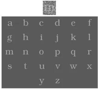
The observer fixates a small black square at the center of the screen. Upon clicking the mouse, the fixation point disappears and in its place a letter (the signal) on a background of static noise is presented for 200 ms and disappears. After a 200 ms delay, the whole alphabet is displayed at 80% contrast. Fig. 2 shows a letter in noise and the whole-alphabet display. The observer is asked to identify the signal letter by clicking a letter in the
whole-alphabet display. The whole-alphabet then disappears and the fixation point reappears. A correct response is rewarded with a beep.
2.3. Orientation discrimination
This task is identical to the letter identification task except that the number of possible signals is restricted to two. We used this task for letters (Sloan font) and gratings (squarewaves and sinewaves). From Sloan we used just the letters and , which are 90° rotations of each other. The gratings alphabet consisted of hori-zontal and vertical sinewaves or squarewaves. All the gratings have Gaussian envelopes (see Section 2.10).
2.4. Detection
Two interval forced choice: after the fixation point disappears, there are two 200 ms intervals of static noise separated by 200 ms. The noise is independent in each interval. The signal is added to one of the two intervals, randomly selected, and afterwards the observer re-sponds by clicking the mouse once if he or she thinks the signal was in the first interval and twice if it was in the second. In the case of grating detection, the signal was a sinewave or a squarewave of a fixed orientation. For letter detection, a new letter is randomly selected from the whole alphabet for each trial. A correct response is rewarded with a beep.
2.5. Threshold
For letters, we specify Weber contrastDL=Lbackground. For gratings, we specify Michelson contrast ðLmax LminÞ=ðLmaxþLminÞ. For noise, we specify rms contrast crms¼hc2ðx;yÞi0:5
x;y, where the angle brackets indicate expected value (over all x;y), cðx;yÞ ¼ ðLðx;yÞ LbackgroundÞ=Lbackground, and Lðx;yÞ is the luminance at location x;y. The contrast energy of a letter is the product of squared contrast and ink area. More gener-ally, energy is the contrast power of the signal, inte-grated over spaceE¼R Rc2ðx;yÞdxdy.
Threshold contrast is measured by 40-trial runs of the modified Quest staircase procedure (Watson & Pelli, 1983; King-Smith, Grigsby, Vingrys, Benes, & Supowit, 1994) using an 82% correct criterion and a b of 3.5. Threshold energyEfor the alphabet is the average letter energy (across all the letters) at the threshold contrast for the alphabet. The reported threshold (log energy) is averaged over several runs.
2.6. Observers
There were 11 observers. Table 1 lists which observers were tested on each type of signal. For each signal type, Fig. 2. Top: a letter at threshold contrast on a background of noise.
Bottom: the subsequently shown high-contrast display of the alpha-bet from which the observer chooses a response. (The right answer is ‘‘m’’.)
each observer was tested at all sizes (spatial frequencies in the case of gratings). For gratings, each observer was tested with both squarewaves and sinewaves.
All observers were fluent readers of literature in the alphabets they were tested on. In the case of the Kuunstler display script, the results of the first 2000 trials€ were discarded before collecting the data reported here. This criterion is based on the finding that efficiency for identifying letters from a new alphabet initially grows rapidly but grows very slowly after 2000 trials (Pelli et al., in press). All the observers had normal or cor-rected-to-normal vision.
2.7. Stimuli
The stimuli were created on a Power Macintosh using MATLAB and the Psychophysics Toolbox (Brainard, 1997; Pelli, 1997; http://psychtoolbox.org). The back-ground (the entire monitor) luminance was set to the middle of the monitor’s range, about 16 cd/m2. The stimulus consisted of a signal added to a background of noise. The noise covered the signal and extended 25% beyond its (invisible) bounding box. The signal was a letter, a filtered letter, or a grating.
2.8. Letters
We used letters from several fonts and alphabets at various sizes. We used the 26 letters of lower-case Bookman and upperlower-case KuenstlerScriptTwo-Bold (K€uunstler) fonts, which are commercially available PostScript fonts from Adobe Systems. The 26-character Chinese font, Yung, was created in Fontographer from scans of calligraphy drawn by Yung Chih-sheng (Pelli
et al., in press). The 10 Sloan characters are specified by the National Academy of Sciences-National Research Committee on Vision (1980). We tested Sloan in its plain and outline styles. 57 is an upper-case font that was commonly used on CRT terminals in the seventies. Yung and Sloan are available from us for research purposes. The retinal size of the letters was varied either by changing the viewing distance or by changing the size of the letter on the monitor. The letters and noise were rendered using uniform square checks of fixed size at either 2 or 4 pixels/side. Table 1shows our fonts and alphabets, and specifies the range of viewing distance, pixel size (deg), letter width (deg), and stroke frequency used in our experiments.
2.9. Filtered letters
For the filtered letters, we followed closely what Parish and Sperling (1991) did. Note that Parish and Sperling took height as letter ‘‘size’’, whereas here we take width as letter ‘‘size’’. The letter size (width) of the 57 font on the screen was 35 pixels. (Height was 45 pixels.) We filtered the letters of the 57 font into six octave-wide bands corresponding to six successive levels of a laplacian pyramid (Burt & Adelson, 1983). We used two of those bands. Band 2 was centered at 1.2 c/letter-width (i.e. 1.5 c/letter-height), and band 4 was centered at 4.5 c/letter-width (i.e. 5.8 c/letter-height). Varying viewing distance from 6 to 384 cm produced letter sizes from 12°to 0.2°.
2.10. Gratings
We used both sinewave and squarewave gratings at various spatial frequencies. Gratings were vignetted by a Table 1
Parameters of the various signals Alphabet Width (deg) Stroke
frequency (stroke/letter) Stroke frequency (stroke/deg) Pixel size (deg) Noise rms contrast Viewing distance (cm) Observers
Sloan 0.18–55 1.6 0.03–9 0.0037–0.20 0.15–0.35 10–550 MCP, IOF, AHC, MLL,
AS, JLL, RS
Sloan outline 13.2 3.2 0.029 0.15 70 MCP
Bookman 0.10–31 1.7 0.06–16 0.0037–0.10 0.15 20–550 IOF, AHC, KCH, MCP
Chinese (Yung) 0.25–15 2.8 0.17–10 0.0037–0.10 0.15–0.3 20–550 RH
K€uunstler 0.16–51 2.6 0.06–17 0.0037–0.40 0.15–0.35 5–550 IOF, AHC, MLL
57 0.18–12 1.6 0.13–8.9 0.0050–0.33 0.15 6–384 MLL
Gratings See text 0.0037–0.20 0.15–0.35 10–550 MCP, MLL, EA, RS, AS,
AM Sloan Sloan Outline Bookman . . . Chinese (Yung) . . . K€uunstler . . . 57
The Sloan row includes identification (observers MCP, IOF, AHC, MLL, JLL, RS) and detection (observer MCP) of the full Sloan alphabet and discrimination of (observer AS). The 57 font was always bandpass filtered. Gratings include sinewaves and squarewaves.
circularly symmetric Gaussian envelope. The 1=espace constant was 1period for sinewave grating detection and 3 periods for sinewave orientation discrimination. For squarewaves the 1=espace constant was always 3 periods.
2.11. Noise
The noise is static, made up of square checks: 22 or 44 pixels. Each check is an increment or decrement sampled from a zero mean Gaussian distribution trun-cated at two standard deviations. The rms contrast of the noise was usually set to 0.15. The power spectral density of a random checkerboard (with stochastically independent check luminances) equals the product of contrast power and the area of a noise check. At a dis-tance of 100 cm, a 22-pixel check subtends 0.041°so the power spectral density N is 0:1520:0412¼3:7 105 deg2
. (Table 1lists the range of rms noise contrasts and pixel sizes used.) The white noise was then high- or low-pass filtered at one of various cut-off frequencies. MATLAB functions were used to fast Fourier trans-form our noise matrix, zero all the unwanted frequen-cies, and invert the fast Fourier transform. Our filtering conditions included the two extremes of no noise and all-pass noise.
The signal, like the noise, is uniform within each check. This was achieved by computing the stimulus image at 1=2 or 1=4 the final size and then expanding to final size by pixel replication.
2.12. Stroke frequency
To measure stroke frequency, we drew a horizontal rule through each letter of the alphabet at half the x -height (of lowercase alphabets) or half the ascender height (of uppercase alphabets and Chinese), and counted the number of lines crossed by the rule. The average count, across letters, is the strokes per letter for that alphabet. To convert that to stroke/deg (i.e. c/deg) we divide by the average letter width. To assess the ro-bustness of this measure of letter spatial frequency, we repeated the above procedure with rules of various heights and orientations. We found that the various estimates of stroke frequency varied no more than 10% from what is reported in Table 1.
A particularly nice way to assess the effect of stroke frequency on channel frequency is to compare results with plain and outline versions of the same font, since this change in style doubles the stroke frequency without affecting size.
3. Results
Critical-band masking characterizes the spatial fre-quency tuning of the channel(s) that mediate a task by
determining which noise frequencies interfere with the performance of the task. Fig. 3 shows a few observers’ energy thresholds for letter identification (and grating detection) as a function of the cut-off frequency of low-() or high-pass low-() noise. We got similar masking functions for all the signals and tasks we tested. As the cut-off frequency of low-pass filtered noise is increased, the threshold begins low at the left, at its no-noise level, and rises monotonically, in a sigmoidal fashion, until it reaches the threshold in white (all-pass) noise at the right. The steepest increase is at the spatial frequencies that interfere most with the task. In high-pass noise, the masking function is similar but mirror-reversed: high at the left, starting up at the threshold in white noise, and descending monotonically to the no-noise threshold at the right. Note that the fits to low- and high-pass thresholds are independent; the asymptotes (thresholds in no and all-pass noise) are not constrained to be equal. For one font and size, Solomon and Pelli (1994) showed that letter identification was mediated by a single spatial frequency channel with a one- or two-octave bandwidth. We have extended that result to all our signals. To derive the channel tuning from the mask-ing functions, we assume that the energy threshold is linearly related to the total power passed by the channel (filter) mediating the task (see Appendix A). The filter’s tuning function is the first derivative of the masking function in either high- or low-pass noise. Of course, the derivative tends to emphasize the variance of the mea-sured thresholds, resulting in noisy tuning curves. Ra-ther than smoothing the curves afterwards, we assume a parabolic form for the tuning (log gain vs. log fre-quency) at the outset and make a maximum likelihood fit of its integral to the thresholds. The fits to the data are plotted as solid (low-pass) and dashed (high-pass) lines in Fig. 3 (top row).
Fig. 3 (middle row) shows examples of channel tuning functions obtained in this way. Since we used both low-and high-pass noise, we got two tuning functions for each signal set (an alphabet of particular font and size). Power gain is plotted as a function of spatial frequency. The functions are normalized to have a peak power gain of 1. We defined bandwidth, in octaves, as the log2of the high-over-low ratio of the two frequencies at which the power gain was 0.5 (i.e. full bandwidth at half height). Appendix B examines the channel bandwidth and the ratio of center frequencies. Both estimates turn out to be too noisy to be of much use.
3.1. Off-frequency looking: choosing the channel
Our first analysis assumed noise additivity for low- or high-pass noise. Our second analysis goes back to the thresholds and tests for additivity of low- and high-pass noises. The dashed line in Fig. 3 (bottom row) plots the sum of threshold elevations in low- and high-pass noise
for each cut-off frequency. If the noises were additive, this dashed line would predict the solid line, which is threshold elevation in white all-pass noise. The summed elevations (dashed line) never fall far below the solid line. The greatest difference occurs at the frequency where the masking functions cross. We took the point of maximum discrepancy for each pair of masking func-tions and computed the ratio of predictedEþ
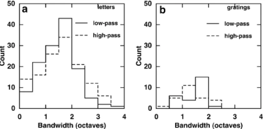
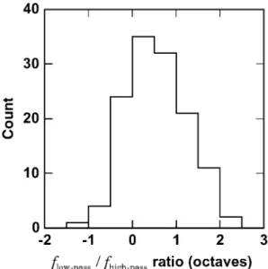
lowþEhighþ to actualEþallthreshold elevation in all-pass noise. Negative values indicate how much better (lower energy thresh-old) the human observer does in filtered noise than ex-pected for a single-fixed-channel model with the same white-noise threshold. Fig. 4 shows histograms of that noise additivity ratio for all kinds of signals used. The geometric mean is 0.17 log unit. A central fea-ture of channel theory has been the multiplicity of vi-sual channels and the opportunity they offer to enhance
sensitivity by choosing the channel(s) with best signal-to-noise ratio. These results show that the observer does hardly any better in noise that is restricted to either side of the signal frequency than one would expect from the threshold in white noise.
This small discrepancy confirms Pelli (1981), who claimed it (and the lateral shift of the tuning function) as evidence for off-frequency looking (channel switching). However, the whole point of switching channels is to see a signal that would otherwise be invisible and this measly 0.2 log unit reduction in threshold energy seems too small to be of any practical importance. (Since energy is proportional to contrast squared, the reduction of log contrast threshold is only 0.1.)
For sinewave signals, which are narrowband, the mere existence of the effect seemed of theoretical sig-nificance (the channel changed), but finding the same Fig. 3. Top row: Energy threshold as a function of cut-off frequency of low-pass () or high-pass () noise. The curves in the top two rows present our first analysis, which assumes noise additivity for low- or high-pass noise. The curves in the bottom row present our second analysis, which tests noise additivity of complementary low- and high-pass noises. In the two top rows, the solid (low-pass) and dashed (high-pass) lines are maximum-likelihood fits based on the assumption that energy threshold is linearly related to the total noise power passed by the channel mediating the task (see Appendix A). Each column of graphs is for a different signal or task: (a) Identification of 5 stroke/deg (0.5°) K€uunstler letters. (b) Detection of 3 c/deg squarewaves. (c) Detection of 2 c/deg sinewaves. (d) Identification of 1.7 stroke/deg (1.7°) K€uunstler letters. (e) Identification of 0.3 stroke/deg (5.5°) Sloan letters. (f) Identification of 6 stroke/deg (0.4°) Chinese (Yung) characters. Middle row: Channel tuning functions derived from the masking functions in the top row (by taking the first derivative). The fits constrained the tuning functions to be parabolas in log power gain vs. log frequency space. The bottom row assesses the observers’ ability to avoid noise by switching channel. The dashed line is the sum of threshold elevations in complementary low- and high-pass noisesEþlowþE
þ
high. The solid line is the threshold elevation in the sum of noises (i.e. all-pass white noise)E þ all. The dashed line consistently drops below the solid line when the cut-off frequency is near the channel frequency, but the effect is measly, a factor of 0.6 in energy threshold (i.e. a factor ofpffiffiffiffiffiffiffi0:6¼0:8 in contrast threshold).
meager effect for letters, which are broadband, indicates that observers are unable to switch channel to any useful degree. Finding the same noise additivity ratio (0.2 log unit) for narrowband and broadband signals seriously undermines Pelli’s (1981) interpretation of this effect as off-frequency looking, since the observer of a broadband
signal ought to benefit much more from channel switching, by looking further ‘‘off frequency’’. The0.2 log unit deviation does show failure of additivity (of complementary high- and low-pass noises) but we suspect the failure is not due to channel switching. As mentioned in Section 1, Burgess et al. (1997) and Fig. 3 (continued)
Fig. 4. Noise additivity ratio for (a) letters, and (b) gratings (sinewaves and squarewaves). The log of the ratio of the sum of threshold elevations in complementary low- and high-pass noises to the threshold elevation in all-pass white noise for gratings and letters. The ratio was calculated where the discrepancy was greatest: at the crossing point of the low- and high-pass masking functions. The ratio evaluates the advantage the observer gains by switching to a channel with better signal-to-noise ratio. Combining results for letters and gratings, the meansd is0:170:14 log unit, with a mode of0.18. The data include 102 signal sets: 6 for sinewaves, 6 for squarewaves, and 90 for letters.
Solomon (2000) found non-additivity for low-pass noise. Detecting sinewaves in one-dimensional noise, Solomon found that thresholds were anomalously low (and less than proportional to noise level) when the low-pass noise cut-off frequency was half the signal fre-quency. Graphs of threshold in low-pass noise as a function of noise cut-off frequency have a sigmoidal shape: see the solid curves in the top row of Fig. 3. The effect of pushing down thresholds in the rising part of the sigmoid is to shift the curve slightly to the right, to higher frequency.
The most parsimonious interpretation of these facts is that the observer uses the same channel in high- and low-pass noise, but manages to discount the low-pass noise somewhat. This could produce the slight (0.2 log unit) discrepancy from noise additivity, and shift the low-pass masking function to slightly higher frequency (0.5 octave higher, according to Fig. 9).
Even though the letters have broad spectra, we must ask whether there is visually useable information in bands other than the one used by the observer. Parish and Sperling (1991), Alexander et al. (1994), and Gold et al. (1999) showed that observers can identify letters filtered to any one of several octave-wide bands. This shows that each isolated band has visually useful in-formation, sufficient for identification. Perhaps observ-ers process lettobserv-ers differently when they are filtered, so that the information used in an isolated band is inac-cessible in an intact letter. As it happens, this is ruled out by the unexpected finding (in ‘‘Sharp-edged signals,’’ below) that, at the right sizes, unfiltered letters are vi-sually identified through a channel with center frequency anywhere in a 6:1range of object frequency.
3.2. Channel frequency vs. stroke frequency
How does letter size affect the center frequency of the channel? We summarize the center frequency of the two channels derived from the low- and high-pass data (like Fig. 3) by reporting their geometric mean as thechannel frequency. In comparing effects of size across alphabets, letter size, per se, is not the right parameter to plot. It is well known that it is the frequency of a grating, not its size (extent) that determines the channel frequency. As explained in Section 1, we characterized letters by measuring their ‘‘stroke frequency’’.
Our results exhibit a dichotomy betweensharp-edged
signals (letters and squarewaves), which have broad spectra, andbandlimitedsignals (filtered letters and sine-waves gratings) which do not.
3.3. Sharp-edged (broadband) signals
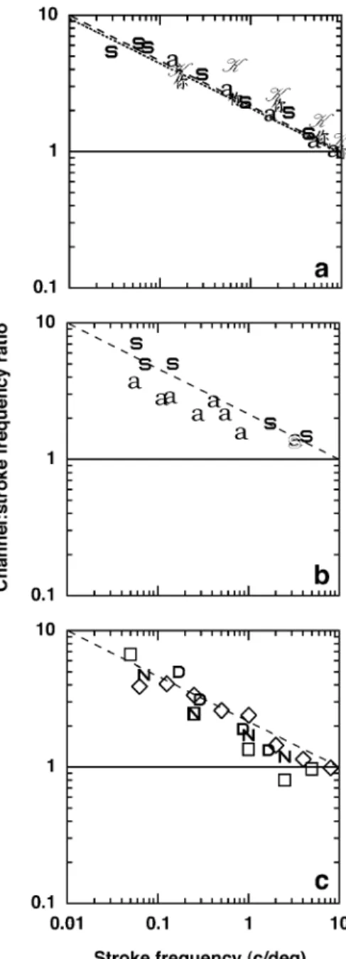
Fig. 5a–c plot channel frequency as a function of stroke frequency for all the sharp-edged signals we used. The data for the various alphabets and squarewaves
superimpose, all falling on or near the dashed line. This result was consistent across all 11 observers. For all of our observers, over the wide range of fonts, alphabets, and sizes we used, stroke frequency was the sole deter-minant of channel frequency. (There are no free para-meters: stroke frequency is a stimulus property and channel frequency is a datum.) For example, outline and plain Sloan both fall on that same channel- vs. stroke-frequency line, even though, at the same size, outline Sloan has twice the stroke frequency as plain Sloan.
The result in Fig. 5a–c is utterly unexpected. All the letter data fall on a single line with a log–log slope of 2=3. If channel frequency scaled with stroke frequency (or reciprocal of size), the data would have a unit slope. Emphasizing that difference, Fig. 6a–c plot the ratio of channel frequency to stroke frequency as a function of stroke frequency. If the channel frequency equaled stroke frequency, the ratio would be 1and the slope would be zero. Instead, the channel-to-stroke frequency ratio diminishes gradually, with a log–log slope of1=3, from 6-fold for the largest letters to 1(a match) for the smallest letters.
These results demonstrate that the visual computa-tion implementing letter identificacomputa-tion is size-dependent. At different sizes, the observer is using different fre-quency components of the letter to identify it. This is illustrated in Fig. 1, where each 8-fold reduction in size results in a 81=3¼2-fold reduction in the object fre-quency (c/letter) used by the observer. We identify large letters by their (high frequency) edges, small letter by their (low frequency) gross strokes.
This result is not unique to letter identification. Fig. 5c plots channel frequency as a function of stroke fre-quency for discriminating between the Sloan letters and , detecting any one of ten Sloan letters, discrimi-nating horizontal from vertical squarewaves, and de-tecting squarewaves. Regardless of signal (letters or squarewaves) and task (detection or identification) the data points all fall on the same dashed line.
We note that in the case of squarewave orientation discrimination the high frequency points seem to lie closer to the equality line. Of course, sine and square wave results must converge at high frequency when the higher frequency harmonics that distinguish them no longer reach the retina (Campbell & Robson, 1968), but this does not account for the convergence seen here at 1 c/deg.
3.4. Bandlimited signals
We also tested bandlimited signals: sinewaves and filtered letters. These results are more or less as expected. A bandlimited signal could only be detected or identified by a channel whose passband includes it, so the ratio of channel to signal frequency would have to be in the range 0.5–2 or so.
We tested sinewaves over a wide range of frequency, 0.05–10 c/deg, and found simple scaling. Fig. 7a plots channel frequency as a function of center frequency. The sinewave channels ( andd) fall along the unit-slope
solid line that indicates equality. Fig. 7b plots the ratio of channel frequency to center frequency as a function of center frequency. Again, there is some scatter, but the sinewave data do not differ systematically from the solid line that indicates equality of channel and signal fre-quency.
Fig. 6. Sharp-edged (broadband) signals. The channel-to-stroke-fre-quency ratio as a function of stroke frechannel-to-stroke-fre-quency replotted from Fig. 5a– c. All the data points lie near the dashed line (- - -) with a slope of1=3,
fchannel=fstroke¼ðfstroke=1 0 c=degÞ 1=3
. The dotted lineð Þ, nearly su-perimposed on the dashed line, is half the critical sampling density reported by Legge et al. (1985), as explained at the end of our dis-cussion.
Fig. 5. Sharp-edged (broadband) signals. Channel frequency as a function of stroke frequency. Channel frequency is defined as the geometric mean of the center frequencies estimated (independently) with high- and low-pass noise (see middle row of Fig. 3). (a) Identifi-cation of unfiltered letters. Each font is plotted using a letter from its alphabet: for Sloan (observer IOF), for Bookman (IOF), for K€uunstler (IOF) and for Yung (Chinese) (RH). (b) Results for other observers: for Sloan (observer AHC), for outline Sloan (MCP), and for Bookman (AHC). (c) Discrimination and detection of un-filtered letters and squarewave gratings. for the discrimination of the Sloan letters and (AS), for the detection of Sloan letters (MCP), squaresfor the discrimination of horizontal from vertical squarewaves (AS) and diamonds}for the detection of squarewaves (MCP). Whether the signals are squarewaves or letters, whether the task is identification, discrimination, or detection, all the data points lie on or near the same line (- - -),fchannel=1 0 c=deg¼ðfstroke=1 0 c=degÞ2=3. This shows that stroke frequency is the sole determinant of channel frequency for all our sharp-edged signals. Results for further observers (not shown) were very similar: Sloan (JLL, MLL, RS, MCP), Book-man (MCP, KCH), K€uunstler (MLL), Squarewaves (AM, MLL, EA, RS).
Some studies that used sinewave grating masks to reveal spatial frequency tuning have argued for a limited number of spatial frequency channels that do not extend much below 1c/deg (Wilson et al., 1983). Our results are
more in line with noise masking studies that reveal channels at frequencies as low as 0.1c/deg (Stromeyer & Julesz, 1972; Stromeyer, 3rd, & Klein, 1982). It is not clear why masking with gratings failed to find the very low frequency channels that are revealed by noise masking.
For filtered letters, the story takes another turn. The letters were bandpass filtered and presented at various sizes (0.18°, 0.59°, 1 .8°, and 5.9° for high-pass letters; 0.18°, 0.59°, 1 .8°, and 11.8°for low-pass letters). TheL’s and H’s in Fig. 7 are the channel frequency for letters filtered to a low- or high-frequency band centered at 1.5 or 5.8 c/letter, respectively. Fig. 7a plots channel fre-quency as a function of the center frefre-quency of the fil-tered letter. The data say three things of increasing subtlety.
First, before reading this paper, one might have ex-pected that channel frequency would equal center fre-quency, regardless of how the center frequency was produced (i.e. a sinewave, or the low band of a small letter, or the high band of a large letter). And, in fact, the data are all within a factor of 3 of the equality line. But that is not the whole story.
Second, consider the isolated effect of size. All theL’s (and all the H’s) have the same filtering (in object fre-quency). Despite some scatter, the L’s follow the unity-slope equality line, and the H’s trace a unit-unity-slope line about a factor of two below the equality line. Similarly, in Fig. 7b, theL’s trace a flat line just below (geometric mean 0.9), and theH’s trace a nearly flat line a factor of two below (geometric mean 0.4) the now-horizontal equality line. Thus, for filtered letters (unlike unfiltered letters), channel frequency does scale with size.
Third, consider the isolated effect of filtering. For each size, the pair of data points representing the low-(L) and the high-(H) pass filtered letters are connected by a dotted line. Since the channel frequency for lowpass letters is at the equality line, and that for the highpass letters is below the equality line, the connecting dotted lines are shallower than the equality line. For each letter size, the observer must be using whatever band the letter is filtered to, but the channel scales less than propor-tionally with the band. Chung et al. (2001) reported a similar result in a different context. They measured the masking effect of a filtered letter on the identification of an adjacent filtered letter. They found a similar fre-quency dependence: at each size, letters filtered to low (or high) spatial frequencies were maximally masked by letters that were filtered to a less low (or less high) fre-quency. For a fixed-size target letter, filtered to various bands, the observer’s channel frequency is a shallow function of the center frequency (averagese log–log slope of 0:50:2 in our small data set, 0.7 in Chung et al., i.e. roughly 2=3 overall). But, as noted above, both in our results and those of Chung et al., if we take a fixed-band (in object frequency) and vary size, then the Fig. 7. Bandlimited signals: filtered letters and sinewaves. The filtered
letters are based on the 57 font used by Parish and Sperling (1991). The letters were bandpass filtered. The L’s are results for letters filtered to alow-frequency octave-wide band centered at 1.2 c/letter (observer MLL). The H’s are results for letters filtered to ahigh-frequency oc-tave-wide band centered at 4.5 c/letter (observer MLL). The sinewave results are plotted as open(MLL) and filled d (AS) circles. (a) Channel frequency as a function of center frequency. The sinewave data are close to the unit-slope solid line indicating equality,
fchannel¼f. The low-frequency-letter data are also close to the equality line (geometric mean offchannel=f is 0.9), but the high-frequency-letter data are below it (geometric mean of fchannel=f is 0.4). A roughly fourfold increase in center frequency (4:5=1:2¼3:8) produced roughly twofold (3:80:4=0:9¼1:7) increase in channel frequency; the aver-age log–log slope of the dashed lines is 0:50:2, which is consistent with the tighter estimate of 0.7 of Chung, Levi, and Legge (2001), so we take 2=3 as an overall summary. (b) The channel-to-center-frequency ratio as a function of center frequency replotted from (a). The sinewave grating (openand filleddcircles) and low-frequency filtered letter (L) results fall near the equality line (––), which now has zero slope. The high-frequency (H) filtered letter results lie below the equality line, as in (a). Results for further observers (not shown) were very similar: Sinewaves (AM, EA, RS).
observer’s channel frequency is proportional to center frequency (log–log slope 1).3
4. Discussion
Before the advent of computers, the best typogra-phers changed letter shape with size (Rubinstein, 1988). Larger letters were given more detail, emphasizing the higher frequency components of the letter, while smaller letters were rendered bolder, emphasizing the lower frequency components. No doubt these shape changes were made to compensate for limitations of both printing and seeing, but they are consistent with our finding of scale-dependence in vision. But how can we reconcile our results with studies that concluded that object recognition, especially letter identification, is scale invariant? Let us review them.
Legge et al. (1985) investigated the visual require-ments of reading by measuring reading rate as a func-tion of several variables. As a funcfunc-tion of letter size, reading rate has an overall inverted-U shape with a wide plateau covering a 60:1range. They also looked at the effects of low-pass filtering and sampling on reading rate. With low-pass filtering, reading rate increases with bandwidth up to 2 cycle/character, independent of size. Based on this result, they suggested that a single spatial-frequency channel sufficed for reading, with the channel scaling with the size of the letter. However, their sam-pling data tell a different story. For optimum reading rate for text seen through a sampling grid, large letters require more samples per character than small letters. Critical sampling density (samples/character) increased as a function of letter size with a log–log slope of 0.3 (i.e. about 1=3). This difference parallels the filtered vs. un-filtered dichotomy in our results, as we will see below.
Parish and Sperling (1991) compared the perfor-mance of human and ideal observers in identifying a filtered letter in filtered noise. They found only a small effect of viewing distance on efficiency, which they at-tributed to the sharp edges of the pixels. In their con-clusion, they dismissed this effect as an artifact of the display and concluded that over their 32:1size range, letter identification was scale invariant.
Thus, like Harmon and Julesz’s (1973) discussion of their blocky pictures of Abraham Lincoln, Legge et al. (1985) and Parish and Sperling (1991) suggested that
letters are masked by the sharp edges of the screen pixels, which are only visible from near. According to them, this masking reduced both the reading rate and letter identification efficiency of large letters because those were studied at close distances.
Alexander et al. (1994) measured threshold for iden-tifying a filtered Sloan letter at two sizes, flickering at 16 Hz. For each size, they bandpass filtered the letters and determined which octave-wide frequency band gave the lowest threshold for letter identification. At a letter size of 0.3 log MAR (9 stroke/deg), the lowest contrast threshold was obtained when the letters were filtered to the band centered at 1.25 c/letter. For a larger letter size of 0.7 log MAR (4 stroke/deg) the best band shifted up to 2.5 c/letter. They concluded that the object spatial frequency (c/letter) of maximum sensitivity increases with letter size.
As mentioned in Section 1, these studies do not resolve the role of size in letter identification. Apparently similar experiments seem to contradict each other. In reading, low-pass filtering the letters reveals a critical bandwidth (2 c/letter) independent of scale, yet reading through a sampling grid shows that more samples are needed to achieve maximum reading rate for larger letters. In letter identification, Parish and Sperling (1991) show that in the presence of noise, optimal performance is achieved when letters are filtered to a band centered at 1.5 c/letter, independent of size. Yet Alexander et al. (1994) report that, without noise, the optimal band shifts to higher object frequency (c/letter) when letter size increases.
Our results describe the role of spatial-frequency channels in letter identification and suggest a framework that provides a coherent account of all the prior work, dispelling the apparent contradictions.
4.1. Letter identification is bottom-up
It is well known that multiple spatial-frequency channels are available to detect and discriminate grat-ings (Campbell & Robson, 1968). Like everyone else, we supposed that channel selection is top-down: the ob-server learns to choose whichever channel(s) are best suited to the task. Furthermore, it seemed quite possible that observers, having read for years, might have de-veloped specialized channels that match the broad spectra of the letters. Or, perhaps, learn to combine information across multiple octave-wide channels.
Having explored a wide range of stimulus conditions (alphabets, fonts, sizes, low- and high-pass noise), we can confidently say that all three of our conjectures, above, are wrong: The channels used to identify letters are not selected top-down, are not broadband, and are not combined across frequencies. Our results confirm and generalize Solomon and Pelli’s (1994) findings for 1°Bookman letters. Firstly, for every task we studied, observers always rely on a single 1:60:7 octave 3
Chung et al. (2001) did not draw attention to this dichotomy, but it is clear in their graphs. Their Fig. 5 shows the 0.7 log–log slope of the best masking frequency as a function of which target band is selected (1.3–3.5 c/letter), and their Fig. 11 replots the same filtered-letters data (gray filled symbols) showing a log–log slope of 1as a function of target spatial frequency (1.3–13 c/deg) when size is varied. (Ignore the other points, which are not for letters, and the shallow line fitted to them.)
channel. Secondly, the choice of channel mediating let-ter identification is delet-termined solely by the properties of the signal, independent of the properties of the noise. (The small0.2 log unit deviation from noise additivity and the small 0.5 octave apparent shift in channel frequency seem better explained as discounting of low-frequency noise rather than as evidence of channel switching.) Although the observers have multiple chan-nels, they persist in using the same channel for the same signal, failing to use different channels for different noises. Our observers were tested in 40-trial runs, with the same low- or high-pass noise spectrum on every trial. We expected the observers to learn to use a different channel, shifting to avoid the noise, but instead, the observers persist in using the same channel, independent of the noise. The channel is selected bottom-up by the signal, not top-down by the observer.
4.2. Edges matter
The rest of our results concern the properties of the signal that determine the center frequency of the channel being used. There is a dichotomy in our results between signals that have sharp edges and those that do not. On the one hand, we have the results for sharp-edged (broadband) signals: unfiltered letters and squarewaves. For these signals, stroke frequency was the sole deter-minant of channel frequency, and channel frequency increased as the 2=3 power of stroke frequency. (A slight exception is that the high frequency squarewave results seem slightly lower and steeper.)
Scale dependence disappeared when we used band-limited signals: sinewaves and filtered letters. With the filtered letters, we independently manipulated the letter size and the frequency content. Both are important in determining the channel frequency. Whether the letter is restricted to a low- or high-frequency band, when only size is changed, channel frequency scales proportionally (log–log slope of 1) with center frequency. However, when a fixed-size letter target is bandpass filtered with various center frequencies, the channel frequency in-creases less than proportionally with center frequency of the target (log–log slope of 2=3, summarizing our 0:50:2 and the tighter estimate of 0.7 by Chung et al. (2001)). In our results (Fig. 7), channel frequency is only 2 higher for same-size letters with 4 higher center frequency.
4.3. Consensus
Let us now re-examine the results of previous studies in light of our finding that the signal, not the observer, selects the channel. As Fig. 1demonstrates, our results confirm the Alexander et al. (1994) finding that the optimal spatial frequency band shifts to higher object frequency (c/letter) when letter size increases.
In their reading experiments, Legge et al. (1985) manipulated the letters in two different ways, producing two different results. Low-pass filtering the letters re-vealed a scale-independent process: observers needed the frequencies up to 2 c/letter to achieve maximum reading rate at every letter size. When they measured reading rate for text displayed behind a sampling grid, they discovered that reading larger letters requires more samples per letter.
Assuming that reading shares the limitation we have found for letter identification, our results provide an explanation for these seemingly contradictory results. In the case of filtered letters (Legge et al., 1985; Parish & Sperling, 1991), the observers used a channel frequency proportional to the signal frequency, so everything scaled. In the case of sampled letters (text behind a grid, Legge et al., 1985) the letters are still sharp-edged so it is appropriate to compare their results with our letter data in Fig. 6a. Plotting their results on our graph, taking half their critical sampling frequency as an estimate of channel frequency, yields the dotted line, indistinguish-able from our results. Thus there is an empirical di-chotomy between results for filtered vs. unfiltered letters, but perfect harmony among published reports.
4.4. Squarewaves
As noted above, we were very surprised to find that channel frequency does not scale with letter stroke fre-quency. One might chalk that up to ignorance––letter identification has received much less attention than grat-ing detection. But it turns out that detection of square-wave gratings yields essentially the same result, falling near the same line as our letter data. Campbell and Robson (1968) built much of their case for channels on a thoughtful comparison of sensitivity (reciprocal of threshold contrast) for squarewaves and sinewaves as a function of size (i.e. spatial frequency). They tried to account for squarewave sensitivity in terms of sensitivity to its component sinewaves. At high frequencies (>1 c/deg) sensitivity to the squarewave equals sensitivity to just its fundamental sinewave component. At low fre-quencies (<1c/deg), sinewave sensitivity falls off, in proportion to frequency, while squarewave sensitivity remains high, about 200, independent of spatial fre-quency. This shows that observers detecting low-fre-quency squarewaves use the higher harmonics, and it was later shown that they do not use the fundamental frequency component (Campbell, Howell, & Robson, 1971; Burr, 1987). This dichotomy violates scaling, showing that detection of low-frequency squarewaves is mediated by detection of the higher harmonics, whereas detection of high-frequency squarewaves is mediated by detection of the fundamental.
It is daunting to realize that we still have not out-distanced the foresight of Campbell and Robson’s