NBER WORKING PAPER SERIES
THE EVOLUTION OF BRAND PREFERENCES:
EVIDENCE FROM CONSUMER MIGRATION
Bart J. Bronnenberg
Jean-Pierre H. Dube
Matthew Gentzkow
Working Paper 16267
http://www.nber.org/papers/w16267
NATIONAL BUREAU OF ECONOMIC RESEARCH
1050 Massachusetts Avenue
Cambridge, MA 02138
August 2010
We thank Aimee Drolet, Jon Guryan, Emir Kamenica, Kevin Murphy, Fiona Scott Morton, Jesse Shapiro,
Chad Syverson, and participants at the INFORMS Marketing Science Conference, in Ann Arbor, Michigan,
the 2nd Workshop on the Economics of Advertising and Marketing in Paris, France, and the NBER
Summer Institute (IO) for helpful comments. We gratefully acknowledge feedback from seminar participants
at the Erasmus University Rotterdam, Goethe University Frankfurt, Hong Kong University of Science
and Technology, London Business School, Stanford University, Tel-Aviv University, University of
California, Los Angeles, the University of Chicago, and Universidade Nova Lissabon. We thank Grace
Hyatt and Todd Kaiser at Nielsen for their assistance with the collection of the data, and the Marketing
Science Institute, the Neubauer Family Foundation, and the Initiative on Global Markets at the University
of Chicago Booth School of Business for financial support. The views expressed herein are those of
the authors and do not necessarily reflect the views of the National Bureau of Economic Research.
NBER working papers are circulated for discussion and comment purposes. They have not been
peer-reviewed or been subject to the review by the NBER Board of Directors that accompanies official
NBER publications.
© 2010 by Bart J. Bronnenberg, Jean-Pierre H. Dube, and Matthew Gentzkow. All rights reserved.
Short sections of text, not to exceed two paragraphs, may be quoted without explicit permission provided
that full credit, including © notice, is given to the source.
The Evolution of Brand Preferences: Evidence from Consumer Migration
Bart J. Bronnenberg, Jean-Pierre H. Dube, and Matthew Gentzkow
NBER Working Paper No. 16267
August 2010
JEL No. D12,L1
ABSTRACT
We study the long-run evolution of brand preferences, using new data on consumers' life histories
and purchases of consumer packaged goods. Variation in where consumers have lived in the past allows
us to isolate the causal effect of past experiences on current purchases, holding constant contemporaneous
supply-side factors such as availability, prices, and advertising. Heterogeneity in brand preferences
explains 40 percent of geographic variation in market shares. These preferences develop endogenously
as a function of consumers' life histories and are highly persistent once formed, with experiences 50
years in the past still exerting a significant effect on current consumption. Counterfactuals suggest
that brand preferences create large entry barriers and durable advantages for incumbent firms, and
can explain persistence of early-mover advantage over long periods. Variation across product categories
shows that the persistence of brand preferences is related in an intuitive way to both advertising levels
and the social visibility of consumption.
Bart J. Bronnenberg
Tilburg University and CentER
Warandelaan 2, Koopmans K-1003
5037 AB Tilburg
The Netherlands
[email protected]
Jean-Pierre H. Dube
University of Chicago
Booth School of Business
5807 South Woodlawn Avenue
Chicago, IL 60637
and NBER
[email protected]
Matthew Gentzkow
University of Chicago
Booth School of Business
5807 South Woodlawn Avenue
Chicago, IL 60637
and NBER
If an intelligent being from a remote planet was presented with certain facts about the trivial physical differences in brands and identical prices which exist in many product categories here on earth and asked to develop a model of consumer choice behavior for these conditions, he might assert with little hesitation that: consumers would be indifferent with respect to the avail-able brands, choice would be a random process, and the market shares for the brands would be equal. (Bass 1974)
1
Introduction
Consumers appear to have high willingness to pay for particular brands, even when the alternatives are objectively similar. The majority of consumers typically buy a single brand of beer, cola, or margarine (Dekimpe et al. 1997), even though relative prices vary significantly over time, and consumers often cannot distinguish their preferred brand in blind “taste tests” (Thumin 1962, Allison and Uhl 1964). Consumers pay large premia to buy homogeneous goods like books and CDs from branded online retailers, even when they are using a “shopbot” that eliminates search costs (Smith and Brynjolfsson 2001). A large fraction of consumers buy branded medications, even though chemically equivalent generic substitutes are available at the same stores for much lower prices (Ling et al. 2002).
Theorists have long speculated that willingness to pay for brands today could depend on consumers’ experiences in the past. Willingness to pay could be a function of past consumption, which could enter expected utility directly (Becker and Murphy 1988), through switching costs (Klemperer 1987), or through beliefs about quality (Schmalensee 1982). It could depend on past exposure to advertising (Schmalensee 1983, Doraszelski and Markovich 2007), or on past observations of the behavior of others, as in Ellison and Fudenberg (1995). At the extreme, brand preferences could be entirely determined by experiences in childhood (Berkman et al. 1997). Under these assumptions, consumers’ accumulated stock of “preference capital” could be a valuable asset for incumbent firms and a source of long-term economic rents.1In Bain’s (1956) view, “the advantage to established sellers accruing from buyer preferences for their products as opposed to potential entrant products is on average larger and more frequent in occurrence at large values than any other barrier to entry” (p. 216).
Existing empirical evidence provides little support for the view that past experiences have a long-lasting
1Throughout the paper, we use “brand preferences” as a shorthand for willingness to pay. We intend this term to encompass
impact on brand preferences. Large literatures have measured the effects of advertising, but these studies often find no effects (e.g., Lodish et al. 1995), and the effects they do measure are estimated to dissipate over a horizon ranging from a few weeks to at most five or six months (Assmus, Farley, and Lehmann 1984, Bagwell 2007). Empirical studies of habit formation and consumer switching costs have been limited to estimating short-run effects using panel data spanning no more than 1 or 2 years (e.g., Erdem 1996, Keane 1997, Dubé, Hitsch and Rossi 2010).
In this paper, we study the long-run evolution of brand preferences, using a new dataset that combines Nielsen Homescan data on purchases of consumer packaged goods with details of consumers’ life histo-ries. Building on Bronnenberg, Dhar, and Dubé’s (2007) finding that market shares of these goods vary significantly across regions of the US, we ask how consumers’ current purchases depend on both where they live currently, and where they lived in the past. This approach allows us to hold constant contemporane-ous supply-side factors such as quality, availability, and advertising, and to isolate the causal effect of past experience on current purchases.
Our data include current and past states of residence for 38,000 households, which we match to 2006-2008 purchases in 238 consumer packaged goods product categories. Our primary dependent variable con-sists of the purchases of the top brand as a share of purchases of either of the top two brands in a category. Consistent with Bronnenberg, Dhar, and Dubé (2007), we show that this share varies significantly across space, with a mean of 0.63 and a cross-state standard deviation of 0.15 in the average product category.
We find strong evidence that past experiences are an important driver of current consumption. We first examine the way consumption patterns change when consumers move across state lines. Both cross-sectional and panel evidence suggest that approximately 60 percent of the gap in purchases between the origin and destination state closes immediately when a consumer moves. So, for example, a consumer who moves from a state where the market share of the top brand among lifetime residents isX% to one where the market share isY% jumps from consumingX% to consuming(.4X+.6Y)%. Since the stock of past
experiences has remained constant across the move, while the supply-side environment has changed, we infer that approximately 40 percent of the geographic variation in market shares is attributable to persistent brand preferences, with the rest driven by contemporaneous supply-side variables. We next look at how consumption evolves over time following a move. The remaining 40 percent gap between recent migrants
and lifetime residents closes steadily, but slowly. It takes more than 20 years for half of the gap to close, and even 50 years after moving the gap remains statistically significant. Finally, we show that our data also strongly reject the hypothesis thatall that matters is where consumers lived in childhood: consumers who move after age 25 still eventually converge to the consumption patterns of their new state of residence.
As a lens through which to interpret these results, we introduce a simple model of consumer demand with habit formation (Becker and Murphy 1988). Consumers in the model are myopic. Their choices in each period depend on the contemporaneous prices, availability, and other characteristics of the brands in their market, and on their stock of past consumption experiences, or “brand capital.” The model has two key parameters: the weight on current product characteristics relative to the stock of past consumption (α), and
the year-to-year persistence of brand capital (δ).
We next present evidence for two key identifying assumptions. The first is that a consumer’s migration status is orthogonal to stable determinants of brand preferences. Panel evidence shows directly that migrants look similar to non-migrants in their birth state before moving, and that age of migration is uncorrelated with purchases prior to moving. As additional evidence, we consider a subset of brands that were introduced late in our sample, and show that where a consumer lived before a brand pair was available does not predict her current consumption. The second assumption is that a brand’s past market share in a given market is equal in expectation to the share today. We introduce historical data on market shares and show that, despite large changes over time in shares, the identifying assumption is approximately satisfied.
Under these two assumptions, we estimate that the weight on current characteristics in utility isα=.62
and that the effect of a given year’s consumption experiences depreciates at a rate of 1−δ =.026 per year.
To shed more light on the economic implications of our findings, we simulate two counterfactual sce-narios. First, we imagine that two brands enter a market sequentially, and ask how difficult it will be for the second brand to equalize the market share advantage of the first. We show that a head start of even a few years creates a formidable barrier, with a second entrant needing to maintain a large advantage in supply-side variables (lower prices, more promotions, etc.) to catch up in the subsequent decade. Second, we introduce a simple model of endogenous firm choices, and use it to study the persistence of brand advantages in the face of idiosyncratic shocks. We show that even with significant noise in the environment, our estimates can easily rationalize persistence of market shares over many decades, as observed in Bronnenberg, Dhar, and
Dubé (2009).
In the final section, we present evidence on the specific mechanisms that underlie our results. We show that the relative importance of brand capital is higher in categories with high levels of advertising and high levels of social visibility. Although we cannot interpret these relationships as causal, they are consistent with a model in which both advertising and observed consumption of peers make the the stock of brand capital more important. At the same time, we observe substantial persistence even in categories where advertising and visibility are low, suggesting that some element of habit formation is likely necessary to rationalize the data. We also assess how much of the geographic variation in shares not explained by brand capital can be attributed to variation in prices, display advertising, and feature advertising.
Our empirical strategy is closely related to work that uses migration patterns to study the formation of culture and preferences. Logan and Rhode (2010) show that nineteenth-century immigrants’ expenditure shares for different types of food are predicted by past relative prices in their countries of origin. Luttmer and Singhal (2010) link immigrants’ preferences for redistribution of wealth to the average preference for redistribution in their birth countries. Atkin (2010) shows that migrants within India are willing to pay higher prices to consume foods that are common in their state of origin. Our results also relate to the literature on the formation of preferences more broadly (Bowles 1998). Our work further relates to the broader literature on sources of entry barriers and incumbent advantages (e.g., Bain 1950, Williamson 1963). In particular, Foster, Haltiwanger, and Syverson (2010) show that the demand curves of manufacturing plants shift out over time, and that a model of endogenous demand-side capital formation similar to the one we develop herein can explain a significant share of older plants’ size advantage relative to newer plants. Finally, our work relates to the conceptual literature on the long term effects of brand equity in marketing (e.g., Aaker 1991, Keller 1993).
Section 2 introduces our data. Section 3 presents descriptive evidence on the evolution of brand pref-erences. Section 4 introduces our model and estimation strategy. Section 5 presents evidence supporting our key identifying assumptions. Section 6 presents estimates of the model parameters, and derives impli-cations for first-mover advantage and share stability. Section 7 presents evidence on mechanisms. Section 8 concludes.
2
Data
2.1 Purchases and demographics
We use data from the Nielsen Homescan Panel on the purchases and demographic characteristics of 48,501 households. The panel is drawn from 50 regional markets throughout the United States and covers purchases made between October 2006 and October 2008, inclusive. Each household receives an optical scanner and is directed to scan the barcodes of all consumer packaged goods they purchase, regardless of outlet. The data thus include purchases not only from supermarkets, but also from convenience stores, drug stores, and so on. The data cover food, beverages, and many non-food items commonly found in supermarkets. See Einav et al. (2010) for a recent validation study of the Homescan Panel.
The most granular notion of a product in the data is a UPC code. Nielsen groups UPCs into categories they call modules. Examples include “canned soup,” “regular cola,” “cough drops,” and “bar soap.” Nielsen also groups UPCs by brand, with Coca-Cola 12-ounce cans and Coca-Cola 2-liter bottles both grouped under the brand “Coca-Cola.” A single brand may span multiple modules. Our raw data include 382 modules and 51,316 brands.
We define the total number of purchases by a household of a particular module-brand combination to be the number of observed shopping trips on which the household purchased at least one UPC in that module-brand. A trip counts as a single purchase regardless of the size, number of units bought, or price paid. In Appendix B we show that our results are robust to alternative quantity measures.
We rank brands within each module by the total number of purchases across all households in the sample. Our main analysis focuses on the top two brands in each module. We refer to the best-selling brand in a module as brand 1 and to the second-best-selling brand as brand 2, respectively.
For each household, we observe a vector of demographics that includes household income, whether the household’s residence is rented or owned, and the household head’s race and Hispanic status.
2.2 Consumer life histories
We supplement the purchase and demographic data with a survey of Homescan panelists’ life histories, which we administered in cooperation with AC Nielsen. The survey was sent electronically to households
in the panel, and we requested that each adult in the household complete the survey separately. The ques-tionnaire asked individuals their country and state of birth, and their current state of residence. For those not currently living in their state of birth, we asked the age at which they left their state of birth, and the number of years that they have lived in their current state. Respondents also reported their gender, their date of birth, their highest level of educational attainment, whether they are currently employed, whether they personally make the majority of the household’s purchase decisions (whether they are the “primary shopper”), and whether they are the “head of household.”
The survey was sent to 75,221 households. From these, 80,077 individuals in 48,951 households re-sponded for a response rate of 65 percent. The surveys were completed between September 13, 2008, and October 1, 2008.
From each household, we select a single individual whose characteristics we match to the purchase data. We first focus on individuals born in the United States. For the set of households with multiple respondents, we then apply the following criteria in order, stopping at the point when only a single individual is left: (i) keep only primary shopper(s) if at least one exists; (ii) keep only household head(s) if at least one exists; (iii) keep only the female household head if both a female and a male head exist; (iv) keep the oldest individual; (v) drop responses that appear to be duplicate responses by the same individual; (vi) select one respondent randomly.
We define a household to be a non-migrantif the selected individual’s current and birth state are the same and amigrantotherwise.
We use the reported birth date to define a respondent’s age, assuming all surveys were completed on September 22, 2008. We define the “gap” in a consumer’s reported history to be the difference between her age and the sum of the number of years she lived in her birth state and the number of years she has lived in her current state. In cases where the sum of a respondent’s reported years living in her birth state and current state exceeds her age (i.e., the gap is negative), we either recode the number of years lived in her birth state to be the difference between her age and the reported years in her current state (if the difference is only one or two years), or drop the household from the data (if the difference is more than two years).
2.3 Additional data sources
We supplement our core dataset with data on the historical market shares of a subset of the brands in our data from Consolidated Consumer Analysis (CCA). These volumes are published jointly by a group of participating newspapers from 1948 to 1968.2 They aggregate results from consumer surveys conducted by the newspapers in their respective markets. For each product category and market, the surveys give the share of consumers who report purchasing each brand.3 We match these brand-category pairs to brand-module pairs in the Nielsen data. We collapse to the state level, averaging each brand’s share purchasing across years from 1948 to 1968 and across markets within states. We then define each brand’s average share to be the share of consumers purchasing divided by the sum of this share across brands within the category.
To interpret our counterfactuals in terms of equivalent price changes, we use aggregate store-level data on 2001-2005 purchases and prices, spanning 30 product categories from the IRI Marketing Data Set (Bron-nenberg, Kruger, and Mela 2008).
To measure module-level advertising intensity, we use data on 2008 advertising expenditures for each module from the TNS Media Intelligence Ad$pender database. We download total expenditures for each top-two Homescan brand in our sample, treating cases where no TNS data exist for the brand in question as zeros. We then sum expenditures by module, and code the top 25 percent of modules by advertising expenditure as “high advertising.”
2.4 Final sample definition and sample characteristics
We exclude modules from the main analysis in which we do not observe at least 5,000 households making purchases. We also exclude a small number of modules in which the top two brands as defined by Nielsen are in fact two varieties of a single brand (e.g., “Philadelphia” and “Philadelphia Light” in the Cream Cheese module). We exclude migrant households for which the gap as defined above is greater than 5 years. For households with a gap greater than zero and less than five years, we set the gap to zero. That is, we assume the age at which the shopper left her birth state was her current age minus the number of years she reports 2From 1948-1950, theMilwaukee Journalis listed as publisher. In 1948, the title isThirteen Market Comparison of Consumer Preferences. In 1949 and 1950, the title isFourteen Market Comparison of Consumer Preferences. From 1951 to 1968, all of the participating newspapers are listed as publisher (the exact set of newspapers varies by year). In 1951 and 1952 the title is
Consolidated Consumer Analysis Information, and from 1953 to 1968 the title isConsolidated Consumer Analysis.
3Until 1958, consumers were asked to report the brand they “usually buy” in each category. From 1959 on, they were asked to
living in her current state. We also exclude individuals with a reported age less than 18 or greater than 99. Our final sample consists of 38,098 households and 238 modules. See Appendix Table 2 for a list of these modules.
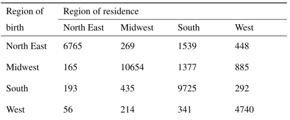
Table 1 summarizes the migration patterns in our final sample. Approximately 16% of respondents are born in a different census region than the one in which they currently live. The most common moves have been out of the Northeast and Midwest and into the South and West regions of the United States.
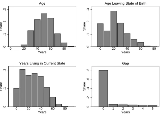
Figure 1 shows the distribution of age of respondents in our final sample, along with the distributions of the age at which respondents moved out of their state of birth, the number of years respondents have lived in their current state of residence, and the gap between the year when they moved out of their state of birth and the year when they moved into their current state of residence. The figure shows that there is substantial variation in all of these measures, and that the majority of sample households have no gap between leaving their state of birth and arriving in their state of residence.
3
Descriptive Evidence
3.1 Measurement Approach
Index consumers byi, modules by j, and states bys. We focus on the top two brands in each category as defined above. Leti’s observedpurchase sharein category j, ˆyi j, be the number of purchases of brand 1 in category jdivided by the total purchases of brands 1 and 2. Let ˆµs jbe the mean of ˆyi jacross all non-migrant
households in states.
For each migrant consumeri, we define therelative sharein category jto bei’s purchase share, scaled relative to the average purchase share of non-migrants in her current and birth states:
βi j= yi jˆ −µs jˆ
ˆ
µs0j−µs jˆ , (1)
wheres0 isi’s current state andsisi’s birth state.
We takeβi jas a summary of the way migrants’ purchases compare to those of non-migrants. If purchases
depend only on contemporaneous supply-side variables like prices, availability, and advertising, migrants should behave identically to non-migrants in their current state and βi j should equal one on average. If
purchases depend only on experiences early in life, migrants should behave identically to non-migrants in their birth state andβi jshould equal zero on average. If preferences evolve endogenously throughout the life
cycle,βi j should fall between zero and one, on average, and should depend on the age at which a migrant
moved and the number of years they have lived in their current state. To look at these patterns in the data, we estimate regressions of the form
βi j= f(ai,ti) +ηi j, (2)
whereai is the age at whichimoved andti is the number of yearsihas lived in her current state. The exact form of f()will vary depending on the specification. Assuming ηi j mainly captures sampling variability
in ˆyi j, its standard deviation will vary inversely with the denominator of equation (1). We therefore weight observations in equation (2) by ˆµs0j−µs jˆ 2.
3.2 Cross-Section
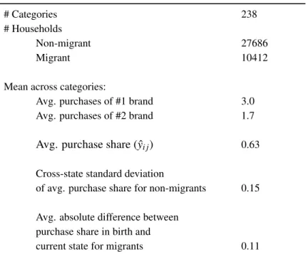
Table 2 summarizes variation in purchase shares. The average of the purchase share ˆyi jacross all consumers
and modules in our sample is 0.63. Conditional on purchasing at least one of the top two brands, consumers
in the typical category make 3.0 purchases of the top brand and 1.7 purchases of the second-place brand. The cross-state standard deviation of the purchase share is 0.15. The absolute value of the gap between the
purchase share in a migrant’s current state and in her birth state is 0.11 on average. These geographic
differ-ences are broadly consistent with the patterns reported in Bronnenberg, Dhar and Dubé (2007). Appendix Table 2 reports the average purchase share and cross-state standard deviation for each module individually.
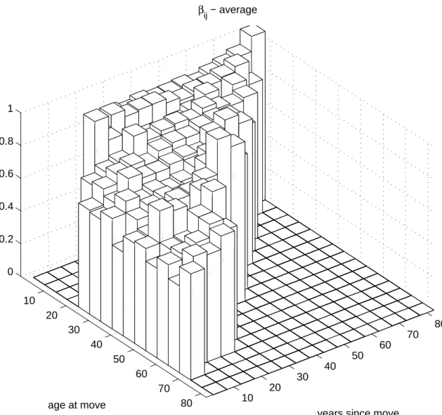
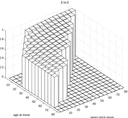
Figure 2 plots the key information in our data: how the relative share,βi j, varies with a migrant’s age
at move (ai) and years since move (ti). We plot estimates of equation (2), parameterizing f(ai,ti) with
dummies for each combination ofai andti, pooled in ten-year bins. The figure shows thatβi j is clearly less
than one on average, rejecting the view that purchases are entirely driven by contemporaneous supply-side variables. It shows thatβi j is clearly greater than zero, rejecting the view that purchases are entirely driven
by childhood experiences. The figure also suggests that the purchases of migrants converge gradually toward those of non-migrants in their destination states.
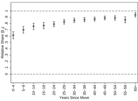
Figure 2 collapsed to two dimensions. Figure 3 shows variation with respect to years since move, pooling across the age-at-move categories. Notice, first, that even very recent movers have relative shares far from zero. This fact suggests that there is a discrete “on-impact” change in purchases at the time an individual moves, equal to approximately 60 percent of the gap between the two states. Referring back to Figure 2, we see that this jump is of similar magnitude regardless of the age at which a consumer moves. Second, note that migrant purchases converge slowly toward those of non-migrants in the years following a move. It takes 25 years for half of the remaining gap in relative shares to close (reachingβi j =0.8), and even after
50 years the difference between migrants and non-migrants remains statistically significant.
Figure 4 shows variation with respect to age at move, pooling across the years-since-move categories. Migrants who moved during childhood have relative shares close to those of non-migrants in their current states, while those who move later look closer to non-migrants in their birth states. This pattern is consistent with the brand capital model we introduce below, which predicts that the preferences of a consumer who has spent more time in her birth state will converge less quickly following a move. It is also consistent with results in marketing that show older consumers consider fewer brands when making a choice and are less likely to switch brands (Lambert-Pandraud and Laurent 2010, Drolet et al. 2008). Interestingly, even consumers who moved before age 5 have relative shares slightly below 1, possibly reflecting the influence of parental preferences on childhood consumption.
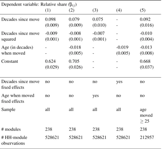
Note that the mechanical correlation between age at move and years since move means that Figures 3 and 4 partly repeat the same information. To separate the effect of age and years, Table 3 presents estimates of equation (2) where we include linear terms inai,ti, andtisquared. To make the coefficients easier to read, we divide bothaiandti by ten. For reference, the first column shows the regression analogue of Figure 3 where we only condition on years since move. The constant in this regression gives the “on-impact” effect of moving, which we estimate to be 0.62. Relative shares start out converging at a rate of 10 percentage points
per decade. The quadratic term is significantly negative, suggesting the rate of convergence slows over time. The second column adds age at move,ai, which we find is significantly negative, showing that the preferences of older migrants indeed converge less quickly to those of their new state even after controlling for time since moving. The third and fourth columns control flexibly for time since move and age at move respectively. The linear and quadratic terms remain strongly significant and similar in magnitude in these
regressions, confirming that time since move and age at move have independent effects.
The final column repeats the regression of column (2) with the sample restricted to those moving at age 25 or later. We present this regression as a further test of the hypothesis that childhood experiences are decisive in shaping preferences. Both the jump on moving and convergence over time remain similar in magnitude and highly significant. So preferences do change, even for those who move late. This result pro-vides some evidence against the common assertion that parental influence is dominant in shaping children’s preferences (e.g., Moore, Wilkie, and Lutz 2002).4
3.3 Panel
Under assumptions we discuss in more detail in section 5 below, the cross-sectional variation in relative shares shown in Figure 2 is informative about how a given migrant’s purchases evolve over time. In this section, we look at within-consumer variation in purchases more directly. The panel dimension of our data is limited, but we do observe a small number of consumers who move during the two years of our sample. For these consumers, we can follow purchases before and after their move, and ask whether the panel lines up with our inferences from the cross-section.
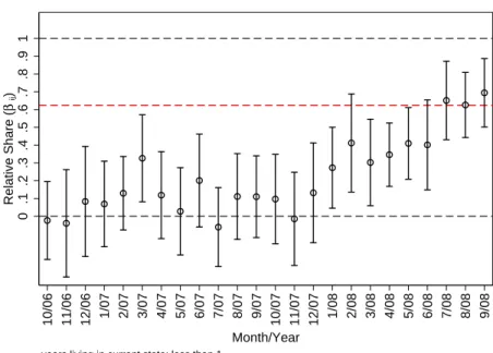
Restricting attention to those for whom the gap between leaving their state of birth and arriving in their current state is zero, we observe 115 consumers who report moving in the past year and 111 consumers who report moving between one and two years ago. Given that our survey was fielded in September 2008, we expect the first group to have moved between October 2007 and September 2008, and the second group to have moved between October 2006 and September 2007.
Figure 5 shows relative shares by month for those who report moving in the past year. Their relative shares for the months up to October 2007 are close to zero, indicating that their purchases before they move are similar to those of non-migrants in their states of birth. If moves are distributed uniformly within the October 2007 to September 2008 period, and if an individual’s relative share jumps to 0.62 on moving, we
should expect the points to increase linearly from zero to 0.62 in the second half of the figure. This pattern
is exactly what we observe.
4Consumer behavior textbooks cite examples of parental influence. For instance, Berkman, Lindquist, and Sirgy (1997) state
that “[i]f Tide laundry detergent is the family favorite, this preference is easily passed on to the next generation. The same can be said for brands of toothpaste, running shoes, golf clubs, preferred restaurants, and favorite stores” (pp. 422-3).
Figure 6 shows relative shares by month for those who report moving between one and two years ago. As we would expect based on the cross-sectional evidence, relative shares increase roughly linearly from October 2006 to September 2007 and then are flat at 0.62 or slightly increasing thereafter.
4
Model and Estimation
As a lens through which to interpret these results, we introduce a simple model of consumer demand with habit formation (Becker and Murphy 1988). The model serves two purposes. First, it allows us to quantify the preference persistence we observe in terms of an economically meaningful structural parameter: the rate at which the stock of preference “capital” derived from past experience decays. Second, it lets us consider the implications of our results for firms’ short-run and long-run demand curves, the importance of first-mover advantage, and the stability of market shares over time.
4.1 Setup
We model a consumer deciding which of the top two brands to purchase in a particular module. We treat states as the relevant product market, assuming that supply-side characteristics of all brands are constant within state. We add subscripts for consumers, modules, and states when we turn to estimation in section 4.3 below.
The difference between the consumer’s indirect utility from the top brand and the second brand is
U=α µ(X,ξ) + (1−α)k−ν. (3)
Here,µ(X,ξ)∈(0,1)is the consumer’sbaseline utility, Xis an observed vector of consumer characteristics,
ξ is an unobserved vector of product characteristics, k∈[0,1]is the consumer’s stock of brand capital, α∈(0,1]is a parameter governing the relative importance of past consumption in current preferences, and
ν∼Uniform(0,1)is a utility shock drawn independently across purchase occasions.
We assume the consumer prefers the top brand to the second brand if and only ifU≥0. The probability that the consumer chooses the top brand (conditional on purchasing one of the top two) is therefore:
y=α µ(X,ξ) + (1−α)k. (4)
Equation(4)is a version of the standard linear probability model of demand (Heckman and Snyder 1997). The baseline utility,µ(X,ξ), captures the influence of all demand factors other than past consumption.
X includes consumer characteristics such as age and income.ξ includes all relevant state-level
characteris-tics of the top two brands, including their prices, availability, advertising levels, and qualities.
The stock of brand capital summarizes the consumer’s past consumption experiences. We define the stock of brand capital to be the discounted average of past purchase shares:
k=∑
A−1 a=1δ
A−ayˆ a
∑A−1a=1δA−a
(5)
where A≥1 is the consumer’s age and ˆya is the consumer’s actual purchase share across all purchase occasions at agea. The parameterδ ∈[0,1]governs the persistence of capital over time.
We assume that equation (3) describes the consumer’s purchases at all earlier ages. We also assume that
α andX are constant; but that the capital stock, k, and the product characteristics, ξ,may have changed over time (for example, because the consumer moved from one state to another). WhenA=1, and thuskis undefined, we assumeU=µ(X,ξ)−ν. We can thus think ofµ(X,ξ)as the expected utility of a consumer who has never before purchased either of the top brands in module j, and so has acquired no brand capital.
It is straightforward to show that the linear recursive structure of equations (4) and (5) means we can writeyas a weighted average of pastµ(X,ξ)plus a mean zero shock:
yA=
A
∑
a=1wAaµ(X,ξa) +εA (6)
whereξais the vector of product characteristics the consumer faced at agea,Eν(εA) =0,wa∈[0,1], and
∑Aa=1wa=1.
Consider, now, the special case in which product characteristics,ξ,vary across states but are constant
over time. It is immediate that if the consumer has lived in the same state throughout her life, her expected purchase share is simply y=µ(X,ξ) +ε, where ξ are the product characteristics in her current state.
agea∗and then moved to a state with characteristicsξ0. It is immediate from equation (6) that
yA=β µ X,ξ0+ (1−β)µ(X,ξ) +εA. (7)
whereβ =∑Aa=a∗+1waAand, hence,β ∈(0,1).
It is straightforward to derive an explicit expression forβas a function of the age at which the consumer
left her birth state (a∗) and the number of years she has lived in her current state (t∗=A−a∗):
β =1−(1−α) " t∗−1
∏
r=1 1− α ∑a ∗+r−1 k=0 δk !# , (8)ift∗>1, andβ =α ift∗=1. See Appendix A for the derivation of equation (8). Note thatlimt∗→∞β =1, and thatβ is increasing int∗. Note also thatβ is decreasing ina∗fort∗>1.
4.2 Discussion
The weight,β,in equation (7) is the model analogue of the relative share defined in section 3: µ(X,ξ)is
the average purchase share among non-migrants in a migrant’s birth state,µ(X,ξ0)is the average purchase
share among non-migrants in her current state, andβ= µ(Xy−,ξ0µ)−(Xµ,ξ(X),ξ).
The predictions of the model are consistent with the facts documented in section 3. A migrant’s expected purchase share falls between the share among migrants in her market of current residence and non-migrants in her market of birth(0<β <1). When an individual moves, a fractionα of the market share
gap between the two markets is closed immediately, as the product characteristics the consumer faces change fromξ toξ0(β=α att∗=1). The parameterα therefore captures the “on-impact” effect of moving. The
on-impact effect is the same regardless of the age at which the consumer moved. The remaining 1−α
portion of the share gap closes gradually over time as her stock of brand capital adjusts. The adjustment is slower ifδ is close to one, and if the consumer was older when she moved (since in this case she has
accumulated a larger stock of past brand experiences).
The model is restrictive in several important ways. First, we only model the relative utilities of the top two brands. We do not model the extensive margin of whether or not to make a purchase in a module at all, and we suppress substitution with other brands.
Second, we assume that the capital stock,k,and the current demand characteristics,µ(X,ξ),are
sepa-rable in the indirect utility function. The influence of prices or advertising on indirect utility, and hence on demand, will be the same regardless of a consumer’s past experiences. The separability assumption delivers the prediction that the jump in relative share on moving (or “on-impact” effect) is the same regardless of the age at which a consumer moves. We make this assumption for tractability, and because it is consistent with the observed data, as seen in Figure 2.
Third, consumers in our model are myopic. We assume the consumer prefers the top brand to the second brand if and only if U ≥0. A sophisticated, forward-looking consumer would take account of the way purchases today will affect her capital stock, and thus her expected utility, tomorrow. Demand would therefore depend not only on current product characteristics, but also on expected future product characteristics.
Finally, we assume that the capital stock is a weighted average of past consumption. As discussed above, past experiences could affect present demand through other channels. Past consumption might matter because of learning, and so enter current demand through beliefs rather than preferences. Past exposure to advertising or past observation of peers might matter independently of the level of past consumption. We see our evidence as potentially consistent with all of these stories and our data do not allow us to distinguish them completely. We specialize to a habit model mainly because it is a simple way to capture the key facts. We consider evidence for advertising and peer effects in section 7 below.
4.3 Estimation
Index consumers byi, modules by j, and states bysas in section 3. Index years byt. For each consumeri, we observe a vector of purchase shares with typical element ˆyi j, a vector of observablesXi, and a vectorMi
which encodesi’s history of migration—her current and birth state, the age at which she moved (a∗i), and the number of years she has lived in her current state (ti∗). We use ˆy,X, andMto denote the matrices which pool these vectors acrossi.
We parametrize baseline demandµ()as:
whereλis a vector of parameters andγjst is shorthand for the valueγ(ξjst)of a function mapping the vector
of product characteristicsξjst to a scalar. The vectorXi includes log income, as well as dummies for age,
Hispanic identity, race, educational attainment, and employment status.
Our first identifying assumption is that there are no unobserved consumer characteristics correlated with both purchases and the exogenous variablesMi andXi:E(yi jˆ −yi j|X,M) =0.
Our second identifying assumption is that, conditional on observables, the expectation of baseline de-mand in a given module-state pair in a past period is equal to the expectation in the current period. Denoting the value ofγjst in the current period byγjs, we assume:E(γjst−γjs|X,M) =0∀t.
For a consumer born in statesand currently living ins0, we then have:
E(yˆi j|X,M) = γjs+Xiλj ifs=s0 β(a∗i,ti∗;α,δ)γjs0+Xiλj+ [1−β(a∗ i,t ∗ i;α,δ)] [γjs+Xiλj] ifs6=s0 (10)
whereγjs denotes the current value ofγjst, andβ(a∗i,ti∗;α,δ)is given by equation (8). Note that we now
allowξjst to vary over time within a market. It is straightforward to show thatβ(a∗i,ti∗;α,δ)is the same as
in equation(8),where we assumed thatξ was constant over time within a market.
We estimate the parameters of this model using a two-step, non-linear least squares estimator. In the first step, we estimate the parametersγjs ∀sandλjfor each module jby running an OLS regression of ˆyi j
onXiand a vector of state dummies using only the non-migrant consumers (for whoms=s0). In the second
step, we estimate the remaining parameters,α andδ,by minimizing[yi jˆ −E(yi jˆ |X,M)]2, holdingγjs ∀j,s
andλj ∀j constant at their estimated first-step values.5
We compute bootstrap standard errors, clustered by module. That is, we sampleJmodules with replace-ment at each iteration, and include all households in each selected module. Our standard error estimates are therefore robust to within-module correlation induced by, for example, variation over time in γjst or
household-module-level unobservables.
5We weight observations equally in our main specification. In Appendix B we show that our estimates are similar if we give
5
Evidence on Identifying Assumptions
5.1 No Selection on Unobservables
Our first identifying assumption is that there are no unobserved consumer characteristics correlated with both purchase shares, ˆyi j, and the observables,Mi andXi.
Of particular concern is the possibility that migrants are selected to have unobserved brand preferences intermediate between the typical non-migrant in their state of birth and their current state of residence. It could also be the case that migrants who stay in a state for many years after moving have characteristics more similar to lifetime residents of that state than migrants who only stay for a few years.
The first test of our identifying assumption is the within-consumer analysis presented in Figures 5 and 6 and discussed in section 3 above. We see that the migrants look similar to non-migrants in their birth states in the months before they move. The mean relative share pooling months 10/06 to 9/07 for migrants living in their current state less than a year is 0.093, the 95 percent confidence interval is(−0.025,0.211), and we fail to rejectβ=0 at the 10 percent level (p=0.12). The data are also consistent with a discrete jump
in migrant purchases on moving. Moreover, purchase shares for these consumers prior to moving are not significantly related to the age at which they moved(p=0.37), providing no support for the hypothesis that
the correlation between relative shares and age at move or years since moving in Figure 2 is primarily driven by selection on unobservables.
As a second test of our identifying assumption, we consider a sub-sample of brands that were introduced relatively recently. Under the assumptions of our model, a migrant who moved before either of two brands was introduced should have an expected purchase share no different from non-migrants in her current state of residence. If the identifying assumption was violated, where a consumer lived before the brands were introduced would be predictive of her characteristics, and so migrants who moved before a brand pair was introduced would look significantly different from non-migrants.
To execute this test, we select pairs of brands that we have confirmed were introduced in 1955 or later. To maximize the power of the test, we do not restrict attention to top-two brands, but include all brand pairs we could identify that were introduced late and have a significant number of purchases in our data. Our final sample includes 52 brand pairs. We compute relative shares,βiw, for each pair was in equation (1), and
estimate the regression βiw= (ω0+ω1ti∗)I(t ∗ i ≤Tw) + [ω2+ω3t ∗ i]I(t ∗ i >Tw) +εiw, (11)
whereTwis the number of years at least one brand in pairwhas been available,ti∗is the number of years
sinceimoved, andI()is the indicator function. We weight observations by µsˆ 0j−µs jˆ 2as in equation (2) above. Under our identifying assumption, we expectω1>0,ω2=1, andω3=0.
Table 4 presents the results. Consistent with our assumption, the coefficient on decades since moving is highly significant for those moving after the pair in question was introduced (ω1>0), but insignificant for
those moving before the pair was introduced (ω3≈0). Moreover, we cannot reject that the average shares of
migrants who moved before the pair was introduced have the same average shares as non-migrants in their current state of residence (ω2≈1). The results are robust to focusing on the complete set of pairs introduced
since 1955, pairs introduced after 1975, and pairs introduced after 1985.
5.2 Expected Past Shares Equal Present Shares
Our second identifying assumption is that, conditional on observables, the expectation of baseline demand in a given module-state pair in any past year is equal to the expectation in the current year.
To test this assumption, we study the 27 modules for which we observe purchases of both current top-two brands in the historical CCA data. For each module-state pair, we compute the current purchase share in the Homescan data across both migrants and non-migrants. We then compare this share to the analogous share in the CCA data for the years 1948-1968, computed as described in section 2.3 above. Under our identifying assumption, we expect that the regression of past shares on current shares should have an intercept of zero and a slope of one.
Note that this prediction would only hold exactly if we compared past and current purchases of non-migrants. We cannot perform this test, because the CCA data do not report shares by migration status. The regression of past on current shares will still be informative, however, so long as migrants are a relatively small share of the population and/or migration patterns have been relatively stable over time.
Figure 7 presents a scatterplot of current versus past purchase shares. Each observation is a state-module pair. The diameters of the circles are proportional to the number of years of CCA data we have for the
observation. The current and past shares are clearly not equal, possibly reflecting real changes in market structure over time as well as sampling variability. However, the fitted values, indicated by the dotted line, are very close to the 45-degree line.
Table 5 presents the corresponding regression of past shares on current shares, weighting by the number of years of CCA data, and clustering by module. The estimated constant is 0.084 and the estimated slope is
0.822. We cannot reject the joint hypothesis that the constant equals zero and the slope equals one (p=0.30).
A possible concern is that the coefficient in this regression may be attenuated by measurement error in the current shares. Consistent with this hypothesis, restricting the regression to state-module pairs where we observe at least 200 households making purchases in the Homescan data increases the estimated slope to 0.926 and reduces the estimated constant to 0.027. Restricting the sample to state-module pairs with at
least 500 households increases the estimated slope to 1.039 and reduces the estimated constant to 0.001.
Together, this evidence supports the assumption that the best predictor of a past purchase share given the data we observe is the present purchase share.
6
Results
6.1 Parameter Estimates
Table 6 presents estimates of the brand-stock model described by equations (4) and (5). The first parameter of interest isα,which represents the “on-impact” effect of moving to a different state. We estimateα =
0.623, which is consistent with our descriptive analysis above and confirms that about 60% of the preference
gap between territories is crossed on-impact when moving. Under the assumptions of our model, it also implies that 60% of the observed cross-state dispersion can be attributed to variation in supply-side factors
ξ. The remainder, about 40% of regional share variation, can be attributed to consumers’ stock of brand
capital.
The estimate of the persistence parameter, δ,is 0.974. This magnitude is consistent with the earlier
evidence that preferences appear highly persistent. The estimates suggest that it takes 26.5 years for half of a given year’s contribution to the capital stock to decay.
9 shows the residuals. The residuals do not show any strong systematic patterns, suggesting the model successfully matches the qualitative features of the data.
6.2 Demand Dynamics
To see what these estimates imply for long-run and short-run price responses, consider a hypothetical market in which the top two brands,AandB, have equal market shares (µ(X,ξ) =0.5). Assume that the market
has the same age distribution as the one observed in our Homescan sample, and that the current capital stock isk=0.5 for all consumers.
Suppose, now, that brandAcuts its price to a level that increases baseline demand,µ(X,ξ), from 0.5 to
0.6.6This change causes an immediate increase in brandA’s purchase share from 0.5 toα0.6+(1−α)0.5=
0.56.
For a permanent price cut, the model implies that the purchase share will eventually rise to 0.6. These
long-run payoffs will take many years to materialize, however. The dynamics of the purchase share follow-ing a permanent price cut will, by assumption, be the same as the dynamics of a migrant’s share followfollow-ing a move, and so will have a path very similar to that shown in Figure 3.
Our model also implies that the price cut will have long-run effects even if it is temporary. Given the estimated parameters, however, these effects will typically be very small. If brandAreverts to its original price after one year, its purchase share falls from 0.562 to 0.501. The long-run effect of the price cut
is thus 1.6 percent of the on-impact effect (although the slight increase will last for a long time). This observation may explain why studies of temporary changes in advertising intensity have generally failed to detect significant long-run effects beyond a horizon of a few months (Assmus, Farley, and Lehmann 1984, Bagwell 2007). It also suggests that the long-run preference formation we are studying here is a distinct phenomenon from the habit effects documented by Dubé, Hitsch and Rossi (2010), where brief price cuts lasting days or weeks have large effects on subsequent purchase behavior.
6.3 Early entry and catching up by the later entrant
In this section, we consider the implications of our findings for first-mover advantage. We simulate a hypo-thetical market in which twoex-antesymmetric brands,AandB, enter sequentially. For a given head start by brandA, we ask how much and for how long brandBwould have to invest to achieve parity in purchase shares.
Let equation (4) be stated in terms of relative demand for brand B, so thaty=0 corresponds to all consumers buying fromAandy=1 corresponds to all consumers buying fromB.
For simplicity, we consider a stylized setting in which the only brand characteristic that enters baseline demand is the allocation of shelf space in retailers. FirmsAandBcan make payments to retailers to give their brands more or less space. The brand characteristicξ is the share of space devoted toB. Since the brands are otherwise symmetric, we assume an inexperienced consumer’s probability of purchasingBwill be equal to its share of space, so thatµ(X,ξ) =ξ.
In Appendix C, we present auxiliary estimates using store-level price and quantity data from IRI that allow us to give an alternative interpretation of our shelf-space counterfactuals in terms of relative price changes. Pooling across 30 categories, we estimate an average demand elasticity of substitution of ∂log(
yA
yB)
∂log(priceApriceB)=
−1.54.
Suppose thatAhas a head start of 5 years. During this period,y=0 as all consumers buy brandA. The accumulated capital stock at the end of those 5 years isk=0. BrandBthen enters and the two firms play a game that determines shelf space allocations. Abstracting from the details of this game, we know that if space allocations are equal (ξ=0.5), we will havey<0.5, andywill converge toward 0.5 but never reach it.
BrandBwill, thus, never achieve parity in the purchase share. IfBhas the majority of shelf space (ξ >0.5),
bothyandkwill reach 0.5 in some finite number of years. The larger isξ, the faster the convergence. We
can therefore ask how many yearsB would need to maintain a certain share of shelf space,ξ, to achieve
purchase share parity.
More generally, we assume brandA’s head start ist∈ {1,5,10,15,25}years and ask how fast the sec-ond firm achieves convergence using a level ofξ∈ {0.55,0.60,0.65,0.70,0.75}. From the estimates in
Ap-pendix C, these shelf-space allocations are equivalent to price discounts of 1−pB/pA∈ {0.08,0.15,0.22,0.28,0.34}.
(destroy-ing some ofA’s capital) and others will be born (with much less of A’s capital). We run the simulations assuming that the age distribution is stable over time and matches the empirical distribution we observe in our Homescan sample.
Table 7 shows the required number of years to catch up. The results show that at the estimatedα and δ,equalizing shares in a reasonable amount of time requires significant investment. IfA’s head start is 5 years,Bwould need to hold 60 percent of shelf space (or discount its price by 15 percent) to reach market share parity in just more than a decade. To catch up in only 2 years,Bwould need to hold three quarters of shelf space or discount its price by more than 30 percent. IfA’s head start were 15 years,Bwould require 23 years at 60 percent of shelf space, or 3 years at 75 percent of shelf space, to reach market share parity.
6.4 Persistence under market shocks
Bronnenberg, Dhar, and Dubé (2009) show that regional share differences in consumer packaged goods industries persist over remarkably long periods of time. Current local shares are strongly predicted by who was the first entrant in a market, even when that entry happened a century ago, few consumers alive remember a time when both brands were not widely available, and the intervening years have seen large shocks to the economic environment such as the growth of supermarkets, changes in real income, wars, depression, and so on.
Our model does not predict how much persistence we should expect to see because it does not endoge-nize firm choices. The previous section showed that a second entrant would have to make large investments to catch up to the first entrant; it does not say anything about whether or not we will see those investments in equilibrium. In this section, we consider a specific assumption under which our model does have strong implications about persistence: complementarity between the stock of capital (k) and current investments in gaining market share (ξ).
In particular, extend the example of the previous section and suppose that supermarkets allocate shelf space in proportion to expected market share. That is, the shelf space allocation in periodtis
ξt = 1
Nt
∑
i yit, (12)is in fact a common rule of thumb for retailers, and one that some argue will be approximately optimal.7 Such a rule will lead intuitively to persistence in shares because a brand that has a lead in the capital stock of experienced consumers will have a larger share of shelf space and consequently be purchased more often even by inexperienced consumers.
We ask how much persistence this dynamic can explain in the presence of shocks to the two brands’ shares in each period. As above, we assumeµ(X,ξ) =ξ, whereξ is the share of shelf space allocated to
brandBand is given by equation (12). Expected purchase shares are:
yit=α ξt+ (1−α)kit+κt, (13)
whereκt is an i.i.d. shock distributed uniformly on[−κ,κ]. Because of transmission through the capital stock,kit,yit depends on both past and present shocks.
We assume an existing market share for the leading brand of 0.75, which has been in place for as long
as consumers live. We fixα=0.623 (our empirical estimate), and simulate the evolution of market shares
for different values ofδ, from 0.974 (our empirical estimate) in steps of 0.25 down to 0.224. We assume
that the parameter governing the shock process isκ=0.05, a number we choose because it is at the upper
end of typical annual share movements in consumer packaged goods.8 We then forward simulate 100 years of evolution for our hypothetical market.
Figure 10 plots the distribution of the market shares in the final year of the simulation across 1000 replications. The first panel shows that when we fix δ at its estimated value (0.974), long-run market
shares remain closely concentrated around their initial value of 0.75, even after 100 years of shocks. The probabilities that market shares are within 10 or 20 share points of their initial value after 100 years are 72 percent and 100 percent respectively. The mechanism generating the persistence is the recency-weighted window of past experiences in the consumer’s brand capital stock. Within this window, shocks tend to cancel out over time. It is, thus, the stock of brand capital that buffers against the reinforcement of demand and supply shocks. The weaker the brand stock, the more market shares are subject to exogenous shocks that
7See, e.g., references in Bultez and Naert (1988).
8Under the allocation in Equation (12), observe that equation (13) can be aggregated toy
t=αyt+ (1−α)Rikitf(i)di+κt,
wheref(i)is the age distribution in the population. Rearranging this aggregation, we obtainyt=Rikitf(i)di+κt/(1−α). Hence, taking into account the allocation rule, the shocks on market shares are uniformly distributed on [−κ/(1−α),κ/(1−α)]≈
accumulate across time. Accordingly, the persistence weakens when we consider lower values forδ and,
effectively, shorten the relevant window of past experiences. The probability that market shares are within 10 share points of the initial values drops from 72% withδ =0.974, to 22% withδ=0.224, which is barely
above the 20 percent one would expect if shares after 100 years attain a uniform distribution. Asδdecreases
towards 0, historical advantages are all but erased.
From this simple simulation, we conclude that our estimates of preference persistence, combined with complementarity between current investment and brand capital, can rationalize stable market shares over long periods of time even in the presence of large shocks.
7
Mechanisms
7.1 Brand Capital
We estimate that 40 percent of current geographic variation in purchase shares is explained by variation in consumers’ brand capital stocks. For tractability and ease of exposition, we have modeled brand capital formation in a habit framework, assuming the current capital stock is a function only of past consumption. As mentioned in the introduction, however, the brand capital stock may be partly a function of other vari-ables, such as past exposure to advertising (Schmalensee 1983, Doraszelski and Markovich 2007), or past observations of consumption by peers (Ellison and Fudenberg 1995).
To provide a first look at the mechanism behind brand capital, we ask how our parameter estimates depend on whether a category has high or low levels of advertising. Recall that we define a category to have high advertising if total expenditure by the top two brands is greater than the 75th percentile among all categories in our dataset. We re-estimate our main model allowing both the weight on brand capital(1−α)
and the rate of persistence in brand capitalδ to differ by advertising intensity.
We also divide categories by the extent to which their consumption is socially visible. We code this measure subjectively. We judge products to be socially visible if (i) they are frequently consumed together with others in social situations, and (ii) they are frequently consumed or served directly from a package with the brand name visible. Products such as beer, soda, chips, ketchup, and cigarettes are therefore coded as socially visible. Products such as baby food, toothpaste, and cold remedies are not socially visible because
they fail criterion (i). Products such as gravy mixes, frozen pasta, and shredded cheese are not socially visible because they fail criterion (ii). See Appendix Table 2 for the module-by-module coding.
As with advertising, we allow both(1−α)andδ to differ by social visibility. Note that the correlation
between the dummy for high advertising and the dummy for high visibility is low, so the sample splits by advertising and visibility should capture independent variation.
Table 8 presents the results. We find that advertising-intense categories have a significantly lower value ofα,and thus a significantly larger weight on the brand capital stock in utility. We cannot interpret this
difference as causal, but it is consistent with the stock of past advertising exposure influencing current willingness to pay above and beyond the effect of past consumption. We find no significant differences in
δ, consistent with the influence of past consumption and past advertising decaying at a similar rate.
We see a similar pattern with social visibility. We find that categories with a high degree of social visibility have a smaller estimatedα, implying greater weight on brand capital. This finding is consistent
with past observations of peer consumption exerting an independent influence on current willingness to pay. We again find no significant difference inδ.
7.2 Baseline Demand
The remaining 60 percent of geographic variation in purchase shares is driven by differences in baseline demand µ(X,ξ). Recall that the source of this result is the observation that when migrants move, their
consumption shifts immediately toward the dominant brand in the destination market, closing 60 percent of the gap in purchase shares. It must be that migrants encounter some combination of lower prices, higher advertising, widespread availability, or other advantages of the dominant brand that lead to this jump in consumption. The results above do not speak to the role of specific supply-side variables, however.
We can use the aggregate IRI data to get some feel for the role of prices, display advertising, and feature advertising. Details of this exercise are provided in Appendix D. First, for each category, we compute the share of cross-market variation in the log difference in purchase shares explained by the following independent variables: (i) log relative prices, (ii) relative display intensity, (iii) relative feature intensity, and (iv) log relative prices, display intensity, and feature intensity together. We then compute the mean and standard deviation of these shares across categories.
We find that the cross-market correlation between relative shares and prices is −0.50 in the average category. The average share of variance explained by prices is 32 percent. Clearly, one reason migrants adjust their purchases immediately on moving is that they encounter lower prices. We find that the cross-market correlation of relative shares with feature and display advertising is 0.44 and 0.42 respectively,
explaining 28 percent and 24 percent of cross-market variation on average. Migrants also encounter more features and displays for the dominant brand. Together, prices, feature, and display explain 49 percent of the cross-market variation in the average category.
If prices, feature, and display are correlated with other market-level product characteristics such as shelf space allocations, however, these regressions will overstate the share of variation explained. To address this issue, we exploit the panel structure of our data. For each category, we regress the log difference in pur-chase shares at the category-market-week level on market and week dummies, plus each of the independent variables above. From each of these regressions, we compute predicted values by multiplying the indepen-dent variable(s) of interest by their estimated coefficient(s). We estimate the share of variance explained by dividing the variance of the predicted value by the variance of the dependent variable. Finally, we compute the mean and standard deviation of the estimated shares across categories.
From these specifications, we estimate that variation in relative prices explains 20 percent of cross-market variation (std.dev.=13 percentage points). Variation in relative feature intensity explains 7 percent
(std.dev.=5 percentage points), variation in relative display intensity explains 11 percent (std.dev.=9.8
percentage points), and all three marketing variables together explain 21 percent (std.dev.=12 percentage
points).
A candidate variable we are unable to measure is shelf space allocation, or availability more broadly. Marketing models used in practice to determine shelf space allocations often recommend that they be pro-portional to market share (Bultez and Naert 1988). To the extent that shelf space exerts a significant effect on consumption, shelf space could explain a significant share of the remaining variation.
Finally, it is possible that baseline demand depends in part on the observed consumption of others. This role for peer effects differs from the contribution to the brand capital stock discussed above. It would imply we might expect to see faster adjustment (higher α) for highly visible categories. As already discussed,
baseline demand, or that this effect is outweighed by their contribution to brand capital.
8
Conclusions
Our results suggest that much of consumers’ observed willingness to pay for brands may reflect the influ-ence of past experiinflu-ences. We estimate that heterogeneity in brand capital explains a substantial share of geographic variation in purchases. Brand capital evolves endogenously as a function of consumers’ life his-tories, and decays slowly once formed. Brand capital can explain large and long-lasting advantages to first movers. Finally, our results suggest that brand preferences play an especially important role in categories with high levels of advertising and social visibility.
References
[1] Aaker, David A. (1991),Managing Brand Equity, The Free Press, New York, NY.
[2] Allison, Ralph I., and Kenneth P. Uhl (1964), “Influence of Beer Brand Identification on Taste Percep-tion,”Journal of Marketing Research, 1(3), 33-39.
[3] Assmus, Gert, John U. Farley, and Donald R. Lehmann (1984), “How Advertising Affects Sales: Meta-Analysis of Econometric Results,”Journal of Marketing Research, 21(1), 65-74.
[4] Atkin, David (2010), “Trade, Tastes and Nutrition in India,” Economics Department Working Paper No. 80, Yale University.
[5] Bagwell, Kyle (2007), “The Economic Analysis of Advertising,”Handbook of Industrial Organization, 3, 1701-1844.
[6] Bain, Joe S. (1950), “Workable Competition in Oligopoly: Theoretical Considerations and Some Em-pirical Evidence,”American Economic Review, 40(2), 35-47.
[7] —- (1956),Barriers to New Competition: Their Character and Consequences in Manufacturing Indus-tries, Harvard University Press, Cambridge, MA.
[8] Bass, Frank M. (1974), “The Theory of Stochastic Preference and Brand Switching,”Journal of Mar-keting Research, 11(1), 1-20.
[9] Becker, Gary S., and Kevin M. Murphy (1988), “A Theory of Rational Addiction,”Journal of Political Economy, 96(4), 675-700.
[10] Berkman, Harold W., Jay D. Lindquist, and M. Joseph Sirgy (1997), Consumer Behavior: Concepts and Marketing Strategy, NTC Business Books, Lincolnwood, IL.
[11] Bowles, Samuel (1998), “Endogenous Preferences: The Cultural Consequences of Markets and Other Economic Institutions,”Journal of Economic Literature, 36(1), 75-111.
[12] Bronnenberg, Bart J., Sanjay K. Dhar, and Jean-Pierre H. Dubé (2007), “Consumer Packaged Goods in the United States: National Brands, Local Branding,”Journal of Marketing Research, 44(1), 4-13. [13] —- (2009), “Brand History, Geography, and the Persistence of Brand Shares,” Journal of Political
Economy, 117(1), 87-115.
[14] Bronnenberg, Bart J., Michael W. Kruger, and Carl F. Mela (2008), “The IRI Marketing Data Set,”
Marketing Science, 27(4), 745-48.
[15] Bultez, Alain, and Philippe Naert (1988), “SH.A.R.P.: Shelf Allocation for Retailers’ Profit,” Market-ing Science, 7(3), 211-231.
[16] Dekimpe, Marnik G., Jan-Benedict E. M. Steenkamp, Martin Mellens, and Piet Vanden Abeele (1997), “Decline and Variability in Brand Loyalty,” International Journal of Research in Marketing, 14(5), 405-420.
[17] Doraszelski, Ulrich, and Sarit Markovich (2007), “Advertising Dynamics and Competitive Advantage,”