Recognizing Microscopic Structures: Dense Semantic Segmentation of Multiple Histopathological Classes using Fully Convolutional Neural Networks

(1)

Master’s Thesis

October, 2016

Recognizing Microscopic Structures:

Dense Semantic Segmentation of

Multiple Histopathological Classes using

Fully Convolutional Neural Networks

Johan Isaksson

supervised by

Anders Heyden

examined by

Kalle Åström

Centre for Mathematical Sciences

Lund University, Faculty of Engineering

(2)

(3)

Abstract

In order to alleviate the financial burden on the healthcare sector as well as relax its employees’ workload, there is a need to introduce novel tools that automate some of the tasks that today are performed manually. Especially pathology poses a problem with few pathologists, demanding manual labour and unneces-sary work on benign tissue. As a response, the DOGS project aims to develop a tool to automate or assist in Gleason grading of histopathological images from prostate biopsies. It is probable that such a tool would benefit from having ac-cess to individually segmented, pathologically relevant objects from the images. Moreover, considering recent advances in deep learning and its frequently im-pressive performance on various image analysis tasks, it is natural to approach this challenge from a deep learning perspective.

This thesis proposes several fully convolutional neural networks to be used for dense semantic segmentation on histopathological images. The networks’ ar-chitectures are all initially based on already proven networks but are modified in various ways to achieve better performance. Being a supervised machine learning task, the ground truth required to train the network has been devel-oped as a part of the thesis. The best-performing network obtained an accuracy of 79.71 % mean intersection over union and the networks presented plausi-bly equaled or outperformed state-of-the-art methods in nuclei segmentation. However, further work is deemed necessary for reaching adequate segmenta-tion performance. Several suggessegmenta-tions for possible future direcsegmenta-tions of work are presented, as well as obstacles that have to be considered moving onwards.

(4)

Acknowledgements

I would first like to thank Anders Heyden for his supervision which, included many valuable suggestions, ideas and considerations. Moreover the amount of freedom you granted in tackling the various challenges arisen during the thesis has been hugely beneficial for my understanding of the deep learning field. Thanks go out to you Kalle Åberg for your suggestion to do a Master’s the-sis within the DOGS project – combining both relevance to my degree and specialization with it serving as my introduction to deep learning; and to you Agnieszka Krzyzanowska for introducing the DOGS project and the pathology and urology department in Malmö SUS to me, providing insight into the diffi-culties pathologists experience and for taking the time to answer any questions I sent your way.

I would also like to extend thanks to Ida Arvidsson for her generous, if somewhat imposed, lending of her office and computer, as well as to Anna Gummeson and Gabrielle Flood for their inspiring previous work on the DOGS project. Special thanks to Tim Isaksson whom, as always, provides excellent feedback on any and all linguistic and stylistic choices I can possibly make poorly. Thank you Martin, Dženan and Erik for perspective.

(5)

1 Introduction

The healthcare sector is under constant pressure to reduce its expenditures and the workload of its employees. Meanwhile, pathologists have to manually ana-lyze great amounts of images as quickly as possible. An automated tool that considerably assists in or performs some of those analyses is therefore highly de-sirable. Yet, due to the complexity of both the images and the analyses, no such tool exists. In an effort to change this,Vinnova, the Swedish state’s innovation

authority, has granted financing to a collaboration between Lund University

andSectra named Digital Pathology for Optimized Gleason Score in Prostate

Cancer, orDOGS. The goal of the project is to develop an image analysis

solu-tion that will increase the precision and decrease the cost of Gleason grading, which is a system to categorize the severity of prostate cancer in a patient. With the vast increase of performance that artificial and convolutional neural networks (ANN and CNN respectively) in machine learning and image analysis has yielded over traditional approaches, it is very probable that such networks will be included in the project’s end product. This thesis is part of the project and investigates a CNN approach to come up with a possible pre-processing step to a final automated tool. More specifically, this thesis proposes CNNs for use in dense semantic segmentation of multiple classes in histopathological images of prostate biopsies.

The report is structured as follows: first, this chapter expands upon and de-scribes the background of the various relevant fields, followed by the aim of the thesis and previous work; second, a chapter about the dataset and the ground truth extraction; third, a chapter going into depths about artificial and convolu-tional neural networks; fourth, a method chapter about detailed implementation aspects; fifth, a results chapter; sixth, a discussion chapter including various con-clusions drawn from the results, points on the limitations of the work, thoughts about future work as well as some ethical quandaries; and seventh, conclusions.

1.1 Background

1.1.1 Gleason grading

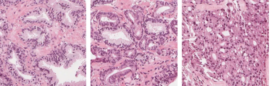
Gleason grading is a histopathological tool with which the grade of prostate cancer can be classified. The assessment is performed by a pathologist through visual analysis of stained microscopy (histopathological) images of either needle biopsies of a prostate in vivo or slices of a surgically extracted prostate. The most common form of staining is with hematoxylin and eosin (H&E), which produces blue, violet and red colorations of the tissue in visible light. In the Gleason Grading system there are five different growth patterns (1-5) that are to be distinguished, each associated with a score corresponding to the pattern number; a lower score indicates a more benign cancer. There are several guide-lines to follow, but in general the patterns range from well differentiated glands to indifferentiable glands: a lower to a higher score, respectively, see Fig. 1.1. 1

(8)

For a given sample the pathologist identifies the two most prominent patterns, or a single pattern twice in the case no other is found, and the combined scores becomes the final Gleason score. This score can then be used for prognosis pre-diction and optimizing therapy.

Figure 1.1: H&E-stained images from prostate biopsies. From left to right, examples of benign, Gleason 3 and Gleason 4 patterns respectively.

Since its introduction in 1966 by Donald Gleason [Gleason, 1966] the Gleason grading system has been modified continuously, with two larger revisions occur-ring in 2005 and 2014, resulting in the gold standard in urologic oncology grading schemes [Trpkov, 2015; Epstein et al., 2016a]. Even so, further improvements are constantly in development and a major overhaul of the system – introducing five separate grade groups – has been proposed in Epstein et al. [2016b] and has re-ceived broad support. The reasoning is that the lower-numbered patterns of the original grading system were products of that day’s less sophisticated methods of analysis; today Gleason pattern 1 is not used at all and Gleason pattern 2 is only identifiable in extracted prostates. This effectively limits the possible Gleason scores (after combination) to range between 6-10, making an objec-tively low score, e.g. 6, sound worse than it is to a patient. The combined score is also problematic, as for example a 3+4 score (Gleason pattern 3 is the most prominent, followed by pattern 4) is significantly less severe than a 4+3 score. These issues makes today’s grading system questionable, especially along with definitions that can be and are interpreted and taught differently between in-stitutions and pathologists – consistency with at most a one-point difference between observers has been reported in 72-87 % of examined cases for a single pathologist in 69-86 % of cases [Trpkov, 2015], see Table 1.1. Nonetheless, even if a new system is implemented the current Gleason system will still remain in use for years or decades before it is completely phased out – and most, if not all, of the inter- and intra-observer inconsistencies will likely persist through to the new system.

1.1.2 Image analysis and semantic segmentation

Image analysis is readily used within healthcare today, in so-called Computer-Aided Diagnosis, for example in radiology. However, the aim is predominantly to detect an ailment, as opposed to detecting its grade – which is the aim in the histopathological field. Beside this task’s increased complexity, the usage of

(9)

Inter-observer observer Intra-Exact agreement 36-81 % 43-78 % Agreement±1 unit 69-86 % _{72-87 %} Table 1.1: Inter- and intraobserver discrepancy

image analysis in histopathology is a considerably newer concept. The reason behind this is that histopathological images are far larger than their radiological counterparts, consists of more color channels and includes several more objects of interest [Gurcan et al., 2009; He et al., 2010]. At the same time, it is esti-mated that pathologists perform 80 % of their examinations on benign tissue. To allow both for more focus on higher-importance examinations and reduce the financial burden on the healthcare sector the workload of the pathologist must therefore be reduced.

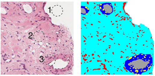
Semantic segmentation is a sub-field of image analysis. Its aim is to extract relevant objects of a given image from the background or other objects and sort them into specific classes. If a cat is to be segmented from the background the end result should consist of an image with pixels with only two discrete values: one correlating to “Cat” and one correlating to “Background”. Semantic segmen-tation can be used as a precursor for further image analysis, such as to allow for feature extraction from a single object in an image. A histopathological example of a segmentation with several classes can be seen in Fig. 1.2. Since this image consists entirely of labelled classes, it furthermore is referred to as a dense segmentation. Segmentation is complex for natural images – on which most work in the field has been done – but it can be argued that segmentation in histopathological images is even more difficult, due to a large amount of objects to be segmented, different tissues and cells that potentially overlapping each other with edges that can be next to indiscernible, as well as pretreatment of the samples and equipment that can result in differing staining characteristics.

1.1.3 Deep learning

Deep learning, or Artificial Neural Networks (ANNs), has become immensely popular in recent years in a wide variety of machine learning fields due to often impressive performance and the ever increasing computational power available. The major difference between deep learning and classical machine learning ap-proaches is that relevant features are devised from the machine itself in the former, while handmade features are used in the latter. This has several advan-tages: the algorithms become more general and an ANN can be used in other instances than originally designed for; the designer does not have to conclude or assume what features are important and which are not; and considerably more complex and a higher number of features become available. There are however two main drawbacks of ANNs: The complexity and combinations of features result in a complicated net whose function – other than its end result – becomes unintuitive and sometimes impossible to comprehend – making designing an adequate net architecture for a given task difficult. Moreover the sheer amount

(10)

Figure 1.2: Example of segmentation of a prostate biopsy sample. To the left is the original image and to the right is the segmentation map. Key: 1. Background, segmented as white. 2. Stroma, segmented as cyan. 3. Ep-ithelial cytoplasm, segmented as blue. The small dark/purple objects in the left image are nuclei. The nuclei in the stroma are colored red and the epithelial nuclei are colored yellow. The white areas surrounded by ep-ithelial cytoplasm are lumen and are colored grey; the epep-ithelial nuclei and cytoplasm together with corresponding lumen constitutes a gland.

of parameters to be trained makes training computationally expensive.

In image analysis, a subset of ANNs called Convolutional Neural Networks are most often used. These follow the same principles as ANNs but are able to retain spatial information throughout their nets. A more comprehensive expla-nation of ANNs and CNNs is found in chapter 3,Deep Learning. CNNs are most

widely used for classification purposes although they have also seen some use in object detection. Using the same analogy as for semantic segmentation, the overall aim of object detection is to recognize that there is a cat, or several cats, in a given image and sometimes their location – but not exactly what pixels it or they consist of. In this sense it can be seen as a less demanding version of semantic segmentation.

A frequent issue is a lack of ground truth for the network to be trained against; research is often performed on recognized datasets, such asImagenetandMNIST.

TheImagenet dataset consists of natural images with annotated classes, such

as e.g. ‘cat’, ‘dog’, ‘person’, ‘car’,; whereas theMNIST dataset provides a vast

array of handwritten digits. For semantic segmentation thePASCAL Visual Ob-ject Classesdataset is popular: it resemblesImagenetas it includes natural

im-ages and the very same classes, but it also offers ground truth for segmentation. Presently, the methods that have achieved the highest accuracy on all of these datasets uses CNNs in some way [ILSVRC2015 Results; Yann LeCun, 2013; PASCAL VOC Challenge]. In histopathology the use of CNNs is less popular, though the amount of research being done is increasing. Work on the segmen-tation aspect is especially scarce and only a handful of articles has been found

(11)

by the author. This could be explained by the fact that semantic segmentation in general using CNNs is a young field – its utilization towards histopathology even more so – and that there is a lack of viable datasets: partly due to how extracting ground truth for semantic segmentation is considerably more time consuming than for classification or object detection [Irshad et al., 2014]. There is, to the author’s best knowledge, only one dataset that offers histopathologi-cal images with a ground truth segmentation: UCSB Bio-Segmentation [UCSB

Bio-Segmentation], the images in which are H&E-stained. However, the dataset only provides segmentation of nuclei. The shortfall of research and datasets notwithstanding, with the results achieved previously with CNNs they have at-tained near-universal acclaim in the entire image analysis field, meaning that further research both utilizing CNNs for semantic segmentation, histopathology, and in combination is certain to be under way.

1.2 Aim of the thesis

This thesis’ aim is to benefit from the state-the-art performance CNNs of-ten produce and perform semantic segmentation on histopathological images of prostate biopsies used for Gleason grading. This is to be done by applying a number of varying CNNs to segment various – and for Gleason scoring rele-vant – tissue types, such as glands, stroma and nuclei, as well as by employing different artificial data expansion techniques to maximize the networks’ perfor-mances. The thesis is meant to act as a stepping stone for further investigations and ultimately assist either the proper automated processing or the pathologists themselves, which in turn could improve the Gleason scoring’s accuracy and con-sistency as well as reduce the workload of pathologists. Since histopathology is a much wider field than just Gleason grading, and due to both the similarities in different histopathological images and CNNs’ inherent plasticity, any promising results in this work could also be applicable in far more settings.

1.3 Previous work

In recent review articles, Gurcan et al. [2009] and Irshad et al. [2014], investigate plenty of traditional approaches for histopathological image segmentation rang-ing in simplicity/complexity. Most of the approaches included use assorted en-sembles of popular algorithms such as thresholding, watershedding, morphology etc. and deal with segmentation and sometimes separation and classification of nuclei, glands, cytoplasm or combinations of these. Both articles note that since there are too few unified benchmarks it is difficult to draw conclusions about how one method compares to another as well as about the overall performance of these methods. An overview of the results nonetheless indicates that tradi-tional methods gives a pixel accuracy for nuclei segmentation in H&E-stained images ranging around 80-90 %.

Long et al. [2015] used a subset of CNNs for use in semantic segmentation called fully convolutional networks (FCNs). Their capability were proven on the Pascal VOC dataset where it achieved state-of-the-art results at 62.2 %

mean intersection over union (IU). This work has since been hugely influen-tial, and network architectures including some form of FCN are nowadays the

(12)

ones predominantly raising the bar in semantic segmentation. Following this, Ronneberger et al. [2015] proposed an “U-net” architecture to segment neuronal structures in electron microscope images as well as track cells over time in trans-mitted light microscope images. The work also employed a number of techniques to artificially increase the available training data. Both FCNs and the U-net architecture will be expanded upon in Sections 3.5,Fully convolutional networks

and 3.5.2,U-networks, respectively. Approaches using FCNs have since been

en-hanced with extra post-processing steps, where the use of Conditional Random Fields after the FCN contributes greatly, reaching 68.7 %, [Chen et al., 2016b], and 73.3 %, [Shen and Zeng, 2016], mean IU for thePascal VOC dataset and

with comparable training data as was used in Long et al. [2015].

The aforementioned reviews mention only few machine-learning algorithms used for segmentation in histopathological images that have been investigated, and none at all using deep learning – which further emphasizes the relative youth of deep learning in histopathology. There does however exist some previous work on this, and as early as 2010 a CNN was deployed to segment nuclei in theUCSB Bio-Segmentation dataset [Pang et al., 2010]. A performance of around 94 %

pixel accuracy was reported with a net of three hidden layers. Further work includes Su et al. [2015], who segmented nuclei clusters in H&E-stained breast cancer images using a “fast” FCN with five hidden layers. Several entries using CNNs were submitted to theGlaS@MICCAI challenge, the goal of which was

to segment and separate colon glands in H&E-stained images [GlaS Challenge Contest]. The winners of the challenge cited the U-net architecture in Ron-neberger et al. [2015] mentioned above as the most relevant previous work for them, and implemented an FCN which performed segmentation and separation of the glands simultaneously with 21 hidden layers [Chen et al., 2016a]. Notably, none of these projects segmented more than one class (which also makes if the segmentations are dense or not inapplicable).

Two works has been concluded thus far in theDOGS project: Gummeson [2016]

and Flood [2016]. Whereas Gummeson used CNNs to automate Gleason scor-ing, thus not being very relevant to this thesis, Flood proposed a branched CNN where the purpose of one branch was to perform Gleason scoring and the other to perform semantic segmentation: the idea being that the segmentation branch would contribute in tuning the common, earlier layers, and in turn boost the classification branch’s performance. In spite of the partially shared segmenta-tion aim between this thesis and Flood [2016], the same dataset has not been used and end results are not comparable. Yet, to the author’s best knowledge, Flood’s work remains the only work on semantic segmentation in histopatho-logical images that both performs dense segmentation on multiple classes using deep learning and is used on prostatic biopsy images.

Again this thesis is the first work known to the author that uses CNNs with the sole aim to perform semantic segmentation in histopathological images to (1) segment multiple (pathologically relevant) classes; (2) to do so densely; and (3) to do so in H&E-stained prostatic biopsy images. It is also the first work that performs dense segmentation using FCNs.

(13)

2 Dataset

In this chapter the dataset used throughout this thesis is described in detail, as well as the methodology for the ground truth extraction.

2.1 Original data

The images for the DOGS project are provided by the Faculty of Medicine

atLund University and Skåne University Hospital. The images considered for

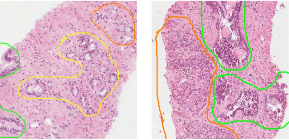
this thesis were exclusively H&E-stained samples from prostate needle biopsies. The samples were digitally sampled using an Aperio CS Slide Scanner with ScanScope software. Samples from several patients were available and areas of benign tissue, Gleason pattern 3-5 as well as other structures had been annotated by a pathologist, see Fig. 2.1. The images have been approved to be used in the DOGS project under ethical permit 2013/400 granted by the Lund University regional ethics committee.

2.2 Data extraction

The images were accessed using the Sectra ISD7 interface, which allowed for

browsing them in all saved magnifications. New images were extracted by using an integrated extraction tool which allowed for user-controlled cropping of a desired, annotated area within the dataset. The cropping border was placed so as to fit the entirety of the annotated area in question, in addition to an unannotated “border” around it, whereupon a TIF file containing several stored magnifications of the cropped area as layers was administered by the software. The layer with the largest magnified version was then saved separately as an uncompressed PNG file. The magnification scale for these images was x20, which translates to a pixel size corresponding to about 0.25µm2_.

2.3 Ground truth segmentation

Unfortunately the annotations provided in the dataset were far too general to be applied for the thesis’ semantic segmentation. The desired ground truth there-fore had to be produced bethere-fore any automatic segmentation could be done. This was immensely time consuming and as a result only half of a single extracted im-age as described above was chosen for manual segmentation. The chosen imim-age predominantly included Gleason 4 patterns intermixed with stroma. Initially the aim was to segment six types of objects: background, stroma, stromatic nuclei, epithelial cytoplasm (EC), epithelial nuclei and lumen. However, as the author lacks pathological training and depended on a few guidelines, some nuclei were hard to discern as stromatic and epithelial. In addition, neither a patholo-gist who was shown some of these was successful in differentiating a few of them, and also pointed out that a couple of the provided nuclei were from other types of cells entirely. In light of this it was decided that instead of separate classes of nuclei, only an overreaching nuclei class was to be used. This has one benefit 7

(14)

Figure 2.1: Example of annotation in the available dataset. Areas encircled in green, yellow and orange correspond to benign tissue, Gleason pattern 3 and Gleason pattern 4, respectively.

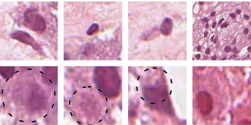
though, as epithelial nuclei is a misnomer: some of them are actually from basal cells – a differentiation that in most cases is impossible to make using H&E-staining. Another issue was encountered with the lumen class: whereas some lumen were straightforward to recognize and segment, others were significantly more troublesome. Ultimately it was deemed that a consistent segmentation of lumen could not be reached. These nuclei and lumen issues are, listed in Fig. 2.2 together with a few additional issues of note.

All segmentation work was done using the image processing softwareGIMP,

ver-sion 2.8.10. The image was zoomed to around 800 % of the original size in order to assess satisfactory segmentation at the individual pixel level. Two marking tools were experimented with: one utilizing manually placed seedpoints and a dynamically alterable threshold based on any color channel or various com-posites, and one applying a threshold-based edge detection between the points. However, due to the varied nature of the individual objects none of these tools proved very useful. Sometimes they were employed to provide a basic segmenta-tion that was subsequently altered by manual pixel colorasegmenta-tion, but the freehand marker tool was instead predominantly used. The individual classes were stored as layers in an XCF file, enabling simple changes both of the desired colors, for visualization purposes, and – more importantly – of which classes to ultimately segment. Lastly, a two-pixel-wide border around each individual object was added: one pixel on the classified objects’ edges and one “outside” the edges. This was done by first creating a new layer and then, for each class, select all object pixels at once, enlarge the entire selection by a constant of one pixel and colorize the result; this effectively created a new “border” class containing objects slightly larger than the individual classes’. This was followed by repeat-ing the initial steps but instead shrinkrepeat-ing the entire selection by a constant of one pixel: resulting in a selection slightly smaller than the individual classes’ objects, and then removing the resulting selection from the border class. The

(15)

Figure 2.2: The various issues with the ground truth segmentation. The top row shows the different nuclei types and lumen aspect: the leftmost image shows a stromatic nuclei below an epithelial nuclei; the second image shows a lymphocyte; the third image shows what is likely a stromatic nuclei left of a monocyte; and the rightmost image shows an example of the difficulty in determining what is and what is not lumen. The bottom row shows additional issues: the leftmost image an example of difficulty where to set the edge of a nuclei; the second image an instance of difficulty in determining if it is a nuclei or not; the third image a tiling artifact with a problematic outcome; and the rightmost image shows a different (redder) saturation than the rest, which was a consistent trait in the rightmost part of the segmented image.

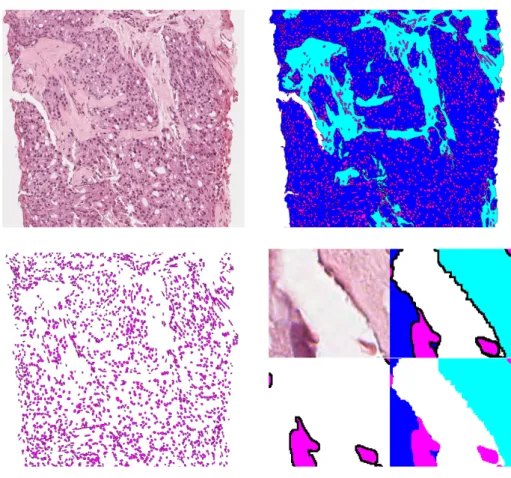
border was produced to account for inconsistency in the segmentation: even though all objects were segmented at the individual pixel level, it is admittedly difficult to know where to place the edges in a consistent manner. Especially background-to-stroma and stroma-to-epithelial-cytoplasm edges were challeng-ing in this regard. The utilized image, final segmentation and an image showchalleng-ing only segmented cells can be seen in Fig. 2.3 and ground truth statistics can be seen in Table 2.1.

Image size 2654x2378

Available classes Nuclei Stroma EC Background

Image percentage (%) 10.9 20.0 49.5 11.1

Nuclei complexes 2128

Table 2.1: Ground truth statistics. The remaining image percentage are the borders. Nuclei are counted as “complexes” since clustered and overlapping nuclei were segmented as belonging to the same object.

(16)

Figure 2.3: The ground truth used throughout the thesis. Top left is the original image; top right is the ground truth with all final classes; bottom left is ground truth with just nuclei; and bottom right is a zoomed-in section of the respective images in addition to one version without borders in the bottom right corner. The classes are denoted as follows, background is white, stroma is cyan, epithelial cytoplasm is blue, nuclei is purple and border is black.

2.4 Data augmentation

It is common practice to artificially expand available ground truth in machine learning applications in order to gain more training data. It is important to consider the exact task that is to be performed when doing this: an image of a car can readily be flipped/mirrored on the horizontal axis and still be sensical, whereas a vertical flip would result in an unnatural example. Beside very basic augmentation techniques such as flipping and rotating an image, different kinds and levels of noise can be added, images can be distorted in various ways and saturation can be altered etc..

Histopathological images are viable for several of these techniques. In contrast to natural images, a rotated histopathological image could still be an unrotated one; mirroring both axes and/or rotating several times over a 360°-span is

(17)

com-monly performed. Because of biological tissues’ inherent variability in size and shape they are also subject to various ways of distortion. Lastly, saturation and noise addition is plausible, since different practitioners and institutions can use different equipment and apply different levels of staining. In this thesis flipping, rotating and distorting the data has been used to augment the ground truth. Saturation and noise has not been altered as all data not only comes from the same institution but the very same sample and image – the existing variety of saturation and noise should be consistent throughout the data – and it should also be noted that data augmentation can increase the requisite training time considerably.

(18)

(19)

3 Deep Learning

This chapter deals with the deep learning background needed for this thesis. It will progress naturally from the most basic parts of ANNs to the complex structures in CNNs and FCNs.

As classification probably is the most popular use of ANNs, and since pixel-wise classification is the aim of this thesis, this chapter concerns ANNs for use in classification exclusively. The goal of any ANN to be used for classification is that it for a given input should produce a desired output, orprediction, in the

form of a class from a select number of classes. If the input are the properties “four legs”, “furry” and “lazy’ the output should be “cat” if the available classes were e.g. “cat”, “elephant” and “lizard”. In this thesis supervised training has been used exclusively; using the same analogy, this would mean that the ANN would be trained by feeding it sets of properties as well as the correct classes (cat dog or lizard). It would then compare its output with the correct class and adjust itself to hopefully produce a better prediction next time.

In practice, the steps above are performed as follows:

1. The inputs are propagated through the network and are affected by various

weights,biases andactivation functions as they pass through them.

2. After the propagation is complete as many outputs as possible classes have been produced in the form of probabilities, and the one with the highest probability will typically become the network’s prediction.

3. The prediction is then compared with the ground truth using aloss func-tion.

4. Depending on the accuracy of the prediction the weights and biases are altered in abackpropagation process.

All these steps are described in their own section below.

3.1 Propagation and artificial neural networks

Artificial neural networks get their names from their conceptual mimicking of biological neural networks. The simplest case is the analogy of a single biolog-ical neuron – prompting a short, simplified description. Neurons are composed of dendrites with synapses, a cell body, an axon and an axon terminal (with its own synapses). The dendrites’ synapses act as the neuron’s inputs from other neurons. These synapse signals are aggregated in various ways among the den-drites, and the resulting signal can either be positive or negative and of varying amplitudes. All dendrites’ signals are summed in the cell body where, if the result has reached a certain threshold, a discrete signal with a neuron-specific amplitude is initiated and passed through the axon. Finally, the signal reaches 13

(20)

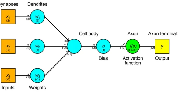
Figure 3.1: Corresponding elements between a biological and artificial neuron. The top labels are for the biological parts and the bottom ones are for the artificial counter-parts. Also note these labels’ variable annotations as well as the operations performed on each interaction. In parentheses is an example of what results the operations give at each step for a set of variables.

the axon terminal where the signal is conveyed from its synapses to other neu-rons. All of these parts and processes has a counterpart in the artificial neuron. An artificial neuron’sinputs are each tied to their own weight, with which all

passing signals are multiplied – an analogy to the dendrites’ synapses and their signal processing properties. All of these weighted inputs are then summed up in thenode: much like the cell body’s function. The result is multiplied with

a bias, where the cell body itself again is the closest analogue, albeit

some-what farfetched. Lastly, the signal is passed through anactivation function –

corresponding to the thresholding the neuron performs before a signal is sent through the axon – before the output is sent on to one or several other node

inputs. Fig. 3.1 shows the connection between neurons and nodes.

3.1.1 Activation function

The activation function is the only non-straightforward aspect here. There are a number of different activation functions that can be used, but networks benefit the most from non-linear functions as they allow for linear separation between

layers(explained in the next section), which in turn reduces the number of layers

needed. Until recently sigmoidals such as the hyperbolic tangentf(x) =tanh(x)

were predominantly used. Today, however, Rectified Linear Units (ReLU) have become the most popular activation function since their relatively low compu-tational load allows for higher layer counts and quicker training [LeCun et al., 2015]. The ReLU is defined as f(x) = max(x,0) and will thus never become

(21)

negative and distort any node whose sum of weights and bias does not reach above 0 – thus fulfilling the required non-linearity.

3.1.2 Networks

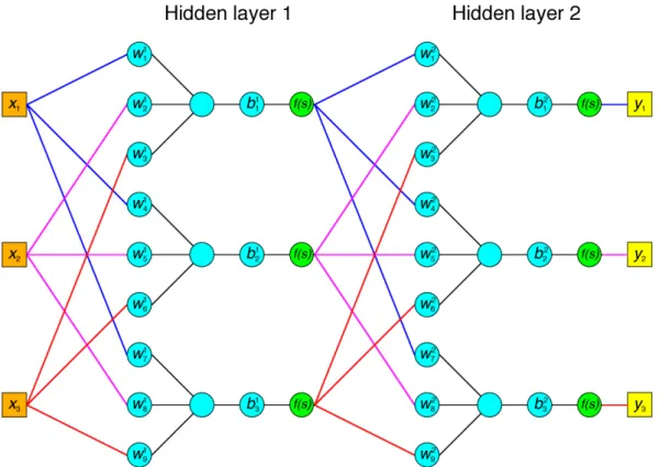
A single neuron often makes for a poor ANN. What is needed is to scale up this simple concept into proper networks with interconnected layers. A layer consists of several neurons, each receiving inputs from the previous layer (or the starting inputs if it is the first layer). If all neurons in a layer receive all the previous layer’s outputs it is called afully connected layer; otherwise it is

called a sparsely connected layer. The neurons in the layer will then process

their respective inputs and pass them along to the next layer (or the end result). This quickly renders it very complex to understand how a given layer or neuron affects the overall network – a major drawback of ANNs. This is also the reason that layers within the network are called hidden layers. The more layers a

network has the deeper it is said to be, and a shallow layer is relatively closer to the input than a deep one. Fig. 3.2 shows an ANN with interconnected layers.

Figure 3.2: An ANN with two fully connected hidden layers with three neurons each. Note that each weight, denoted with its layer in superscript and index in subscript, takes a single input and also that the number of outputs from the previous layer does not limit how many neurons the next one can have.

(22)

3.2 Prediction

The last layer in an ANN is usually reserved to the prediction layer. This layer will output as many values as there are classes. The class with the highest value translates to the network’s prediction. Usually these outputs are normalized so their summed value becomes one, allowing for an intuitive percentage readout of the result. This is done by employingsoftmaxas the prediction layer’s activation

functions. The softmax function is defined as

yi =

ezi

PC j=1ezj

,

whereyidenotes the probability for classi,zthe pre-activation function output, andCthe amount of classes.

3.3 Backpropagation and learning

3.3.1 Accuracy and loss function

In order to penalize erroneous predictions a loss function is employed (“loss”, “error” and “cost” functions all relate to the same concept: the “loss” terminol-ogy is used throughout this thesis). One could just use the network’s missed prediction over total predictions, but a better approach takes into account how close a prediction was to being correct, or conversely with how large a margin a correct prediction was made. The most common way to achieve this is to use the negative logarithmic of a variant of the softmax function, also known as the cross-entropy error, l(x, c) =−_log e xc PC i=1exi ,

where l(x, c)is the loss function with the vector x corresponding to the class

outputs andcto the ground truth class. The loss function’s output is commonly

referred to as the network’sobjective error.

3.3.2 Gradient descent

Given a loss function it is a natural aim to try and minimize it in order to improve the network’s accuracy. If an example of input data is denoted xi,

the current parameters of the networkw, andf(xi,w) =z, from the softmax equation above, the network’s average loss over nexamples of input data can

be written as L(w) = 1 n n X i=1 l(f(xi,w), ci),

which should be minimized overw. It is intuitive to do this by computing the

derivative of w and determine its fastest descent, and this so-called gradient descent approach is indeed what is performed in practice. If e+ 1denotes the

(23)

nextepoch – one cycle of training over the entire training dataset – this looks

like

we+1=we−ηe+1

δf δw(we).

Here,η denotes thelearning rate: the size of the step to be taken in the

direc-tion of the fastest descent. Asw is the entire set of the network’s parameters,

it is implied above that the derivative has to be computed at each layer. In practice, the great dimensionality of ANNs makes this highly computationally expensive. However, as the layers are connected in a prearranged, known order, the chain rule of determining derivatives can be utilized. A layer’s parameters’ derivative can thus be readily computed if the next layer’s parameters’ deriva-tive is known. Hence, if the derivaderiva-tive from the last layer is computed first, it is possible to backtrack through the entire network and benefit from the fact that the “next” derivative is always known – vastly reducing the amount of compu-tations needed. This algorithm is calledbackpropagation. Backpropagation is

used in practically all ANNs, and since the equations it depends on as well as implementation details are easily accessed online they will not be discussed in this thesis.

3.3.3 Stochastic gradient descent, momentum and weight decay

When performing training on an ANN the use ofbatches is usually employed.

That means that the training dataset is split into a number of groups on which the network is evaluated – and its parameters updated – subsequently. This approach both conserves memory and can lead to fasterconvergence: the

net-work has in a sense reached its maximum potential accuracy. It is possible to reduce the time to convergence further, especially in large networks, by using

stochastic gradient descent: a single random training example from a batch is

evaluated before the network updates and moves on to the next batch. The convergence will not be as optimal as in regular gradient descent, but it is often close enough to be considered beneficial overall. Another common way of reach-ing convergence earlier is by applyreach-ingmomentum, which simply adds a fraction

of a particular weight’s previous update to the next one. Both momentum and stochastic gradient descent also have the added benefit of avoiding getting the network stuck inlocal minima; the global, or at least a better local, minimum

is more likely to be found, yielding better accuracy.

Aside from convergence, there is also a desire to avoid overfitting a network.

Overfitting is the case when a network becomes too specialized on the training data: resulting in better accuracy in that context, but worse on the test data. This can be mitigated by reducing the complexity of the network, which in turn can be accomplished by employingweight decay. In practice weight decay means

that large weights will be penalized, effectively promoting weights with small values. If the momentum factor is denotedmand the weight decay factorλthe

gradient descent with weight decay and momentum can be written as

we+1=we(1−λ)−ηe+1

δf

δw(we) +mwe−1.

(24)

3.4 Convolutional Neural Networks

Convolutional neural networks are a subclass of ANNs. They enjoy the prop-erty of retaining spatial information throughout their layers and are therefore especially suited for image analysis tasks. This advantage stems from the nodes each having a filter with which their respective inputs are convolved, rather

than having separate weights as in ANNs. The output will, as in the ANN case after the weighted sum, pass through an activation function before con-tinuing its propagation through the network. A few other types of nodes used commonly in CNNs are explained in the following sections. Depending on the purpose of the CNN, its output can range from a set of probabilities for each possible class, as was the case for the ANN above; or, as for this thesis, a set of probabilities for each possible classfor each input pixel. Thus, by choosing the

most probable class at each pixel, a prediction of a segmented image is produced. With respect to the thesis’ aim, and its relation to image analysis, only two-dimensional filters are relevant for the convolutions, though the filter dimen-sionality can be arbitrarily large in theory. As such, it is also implied that the inputs to the convolutional neurons are two-dimensional. The outputs will in the vast majority of cases therefore also be two-dimensional. With this implica-tion the input to (and outputs from) each layer can be seen as matrices stacked onto each other, giving them three dimensions: height, width and depth. If an input image has three color channels (e.g. red, green and blue) each depth level corresponds to one color channel. Because convolution can be seen as a feature extraction operation, the depths of a convolutional layer’s output are what are often called feature maps. Hence, for the input image the color channels are

equivalent to feature maps. Further on, referring to the dimensionality of lay-ers’ inputs and outputs in general will encompass their height, width and depth. When discussing CNNs, layers are not perfectly corresponding to their ANN counterpart. Instead a set of convolutional filters is referred to as a convolu-tional layer whilst a set of activation functions are called aReLU layer (if it is

in fact ReLU that is used) and so forth. Being faithful to this terminology, each of the layer types used throughout this thesis are detailed below.

3.4.1 Convolutional layers

This section delves into more detail about convolutional layers. A convolution in one dimension is defined as

x(n)∗g(n) =

I X

i=−I

x(m)g(n−m),

wherexis the input in form of a set of samples,gis a weighting function,nis

the sample index andM is the amount of elements in g. This is the discrete

version of convolution; the continuous version will not be discussed in this work as it is not relevant. In two dimensions the convolution becomes

(25)

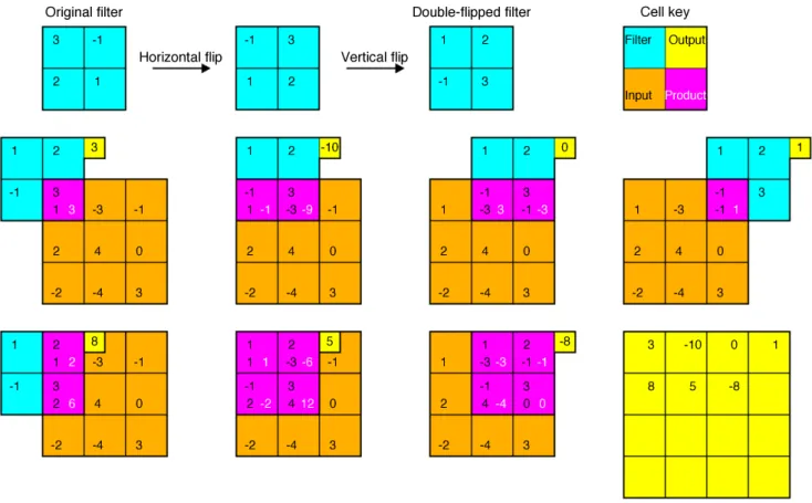
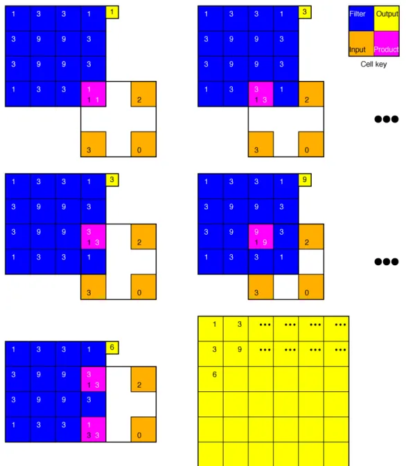
Figure 3.3: Convolution in two dimensions using a 2x2-sized filter and double-flipped 3x3-sized image. The yellow grid shows the result of the seven convolution steps shown. The filter is moved one step at a time, or with astride of one, column-wise. When it reaches the end of a column it repeats on the next row. Note

that some convolutional steps are performed with the filter only partially overlapping the image; it is implied that the cells out of bounds are given zeros as products. This is called zero padding and is optional. In this case it leads to an output larger than the input image – which is typically avoided – but if a 3x3-sized filter is used and there is one extra padded zero around the input image the result will retain the input’s size.

x(n, m)∗ ∗g(n, m) = I X i=−I J X j=−J x(i, j)g(n−i, m−j),

wheren, mdenotes an element at row nand columnm, I the amount of rows

andj the amount of columns in g. g in this case is commonly referred to as a

filter. In practice, this convolution is equivalent to moving the center element of the double-flipped (both horizontally and vertically) filter over each element in the input, summing the product of each overlapping element between the input and the resulting filter, and recording the final result as the output, see Fig. 3.3. Since the convolution operation applies the filter step-wise over the entire image one important property of the convolutional layers is that they are translational

(26)

invariant: meaning that it does not matter exactly where an object is in an image. A convolutional layer produces one feature map per filter chosen to be used: if 64 filters are chosen 64 feature maps will be produced, regardless of the amount of input feature maps. The input depth does, however, control the filters’ depth, or amount of channels. A filter’s depth is simply the same filter stacked onto itself several times. Each filter channel is then used to convolve a single input feature map and when all channels in the filter have convolved their corresponding feature map their respective outputs are summed. The result becomes one of the layer’s outputted feature maps.

3.4.2 ReLU layers

ReLU layers act as the convolutional layers’ activation functions, working in the same manner as the ANN version. The only difference is that a ReLU layer will take the entire feature maps as inputs and apply the ReLU operation to each individual element; the output will hence have the same dimensions as the input.

3.4.3 Max-pooling layers

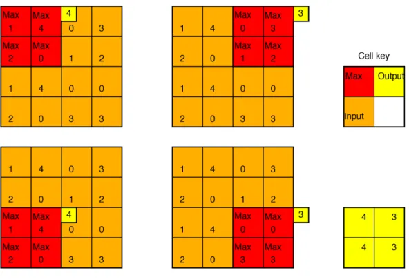
A counterpart for the max-pooling layer was not introduced in the ANN sections. Both because of neural networks’ computational load and the inherent data size of images, it is often desired to reduce the amount of required computations and memory used throughout the network. This can be done with max-pooling layers. The concept entails to simply slide a window over the input feature maps and output the largest value in the window for each step on a new feature map – thus vastly reducing the amount of data used later in the network, see Fig. 3.4, while the amount of feature maps still remain constant. There are other ways to pool feature maps, such as average-pooling layers, but these are not discussed further nor used in this thesis.

3.4.4 Deconvolutional layers

Deconvolutional or, more technically correct, convolutional transpose layers are commonly used to upsample a set of feature maps to higher dimensionality. This is useful in the semantic segmentation case as the pooling layers have previously reduced the dimensionality although the end result should be kept the same size as the input image. Whereas convolutional layers can downsample their inputs if a stride >1 is used, deconvolutional layers upsample when so is the case: a stride of 2 correspond to a doubling of the inputs’ dimensions, see Fig. 3.5. If thus used, they can be seen as a mirrored pooling operation, but being inherently convolutional they can produce any number of output feature maps.

3.4.5 Fully connected layers

Fully connected layers is a layer class where each neuron is connected to all input elements and produces a weighted sum of them. Simply put they are a regression back to the ANN case as there – beside the “external” activation function in the CNN case – is no difference between an ANN fully connected neuron and a CNN one. As a result fully convolutional layers lose any spatial

(27)

Figure 3.4: Example of max-pooling with a 2x2-sized window. In this case, the output’s size is halved in each dimension and the amount of data stored is reduced by the square root of the original’s. Note that the window has a stride of two in order to not include any previously used values. If the input’s height or width dimension is uneven zero padding is often employed to receive an output size of an exact integer division +1 of the input size (a 5x5 input would become a 3x3 output.

information left in the feature maps. This can seem odd recalling that keeping spatial information is a positive trait inherent to CNNs, but in classification tasks where an input image as a single entity should be classified there is no incentive to give the final prediction spatiality. This, in combination with the fact that fully connected layers can extract features on a global level, makes them suitable for use in networks with such classification purposes and are then placed at the very end before the loss layer. They are not employed in any networks used in this work, but they are important to be aware of in order to understand the distinction between FCNs and CNNs, which will be explained in Section 3.5Fully convolutional networks.

3.4.6 Drop layers

Drop layers is a tool to reduce overfitting. By randomly severing connections between feature maps from one layer to weights or filters in the next when train-ing networks they are able to keep the filters and weights generalized: classes will have to rely on a more differentiated set of filters throughout the network. They do however significantly increase the convergence time when training.

(28)

Figure 3.5: Example of upsampling. Upsampling using convolutional transpose is equivalent to convolving the zero-padded input with a number of added zeros between the pixels corresponding to the stride – and in turn the upsampling rate. In this example the convolution is done with a square bilinear filter (unnormalized for the sake of clarity) of size 4x4 and a stride of 2 on an input feature map of size 2x2. The result is a linearly interpolated output of size 6x6. A cropping operation which removes the outmost pixels is often performed directly afterwards to make the resulting output’s size an exact integer multiplication of the input’s – again, mirroring pooling.

(29)

When testing, using drop layers would be detrimental to the prediction and are therefore completely bypassed.

3.4.7 Sum layers

Sum layers simply add a set of feature maps with another of the same dimen-sions. The output will be of the same dimensions, including depth, as the individual inputs. They are inherently an approach to combine two separate layers’ outputs and as such are limited for use indirected acyclic graph (DAG)

networks: which basically are networks that do not consist of a simple chain of layers from the input to the output. One usage of sum layers is presented in Section 3.5,Fully convolutional networks.

3.4.8 Concatenation layers

Another way of combining different layers’ outputs is with concatenation layers. As the name implies, these simply concatenate the feature maps from two inputs. The two sets of maps have to have the same height and width, and the result will as well, but its depth will of course be the two inputs’ added amount of feature maps. As the sum layers, concatenation layers are only used in DAG networks. An example is presented in Section 3.5.2,U-networks.

3.4.9 Loss layers

Loss layers are CNNs’ loss function, simply performing the chosen algorithm, such as cross-entropy error, on the input. In contrast to the ReLU layers, which applied ReLU to each individual element of the input, loss layers will perform the given algorithm on a stack of the same input pixel from each depth and produce a single-depth matrix with the same height and width as the input feature maps. The sum of the matrix gives the objective error between the prediction and the ground truth for an input image; the objective error is not limited to range between 0 and 1. As this layer is the connection between network and ground truth its input should have the same depth as the amount of classes available.

3.4.10 Prediction/Accuracy layers

Prediction or accuracy layers provide the network’s prediction for an input im-age. At each pixel stack from its input they simply choose the element with the highest value and produces its depth’s corresponding class as that pixel’s output. They can also produce metrics of how well the network performed.

3.5 Fully convolutional networks

Fully convolutional networks are a subclass of CNNs and are not to be confused with the fully connected term discussed earlier. In fact they are practically defined as a CNN lacking fully connected layers. Only feature maps are

out-putted, no individual values, and in so the network retains spatial information throughout the entire propagation. This makes them especially apt for semantic

(30)

segmentation tasks, as spatial information remains relevant even in the predic-tion, and makes it easy to produce a prediction with the same height and width as the input image.

3.5.1 FCNxs

As mentioned in 1.3,Previous work, FCNs were made popular in the semantic

segmentation field by Long et al. [2015]. The networks proposed were named “FCNxs”, where the x was replaced by the upsampling rate performed at the very last upsampling layer. The design process behind this net was to take existing CNNs that had performed simple classification well and expand it with an upsampling part at the end. Long et al. first used a network that just upsampled the very end, or the bottommost 21-channel prediction layer, to the original input image resolution. This provided a dense output segmentation map. With the reasoning that classification became more accurate with each downsampled step, but at the cost of worse spatial resolution – resulting in an accurate class-wise but coarse output – they interconnected the network between earlier downsampled levels and the aforementioned prediction layer (making the CNN a DAG CNN in the process). This connection was made by adding separate predictive layers after max-pooling layers which was then additively merged with the old predictive layer. This was done iteratively twice, initially connecting the penultimate downsampled level with the prediction layer before – again – upsamling it to the original image’s resolution, whereupon doing the same with the downsampled level a further step “above” the last connected one. The resulting network is seen in Fig. 3.6. This network did indeed provide both accurate classification and fine segmentation output and each iteration of an added interconnected path resulted in better segmentation performance.

3.5.2 U-networks

Building upon the insights gained in Long et al. [2015], Ronneberger et al. [2015] designed a U-network to perform semantic segmentation. The thought process was the same: to use the classification performance of highly downsampled lay-ers in combination with the retained spatial resolution of earlier downsampling layers. Ronneberger et al. differ in their implementation however, with the U-network having an “expansive” path to mirror the “contracting” path that they and Long et al. shared, instead of the less complex approach of just summing and upsampling different levels as before. This expansive path includes the same amount of convolutional and ReLU-layers as the contracting path, supposedly allowing for spatial information – retained with the use of concatenating layers between upsampling layers and the corresponding level in the contracting path – to be integrated with the contextual information gained at the lower levels. This implies that the upsampling path also include trainable layers. The network is shown in Fig. 3.7.

(31)

Figure 3.6: FCN8s: The best performing network in Long et al. [2015]. Each block correspond to one or two

layers according to the legend. The y-axis maps the downsampled levels with the tick labels corresponding to the amount of times the original input resolution has been downsampled. The number on each block corresponds to its output’s depth; for convolutional layers this also responds to their amount of filters. Nearly all of the network’s convolutional layers use 3x3-sized filters and all include a bias – a typical convolutional layers thus has (3∗3 + 1)∗amount of filters parameters to train. Downsampling is performed with max-pooling layers and at each downsampled level the amount of feature maps are doubled – this, along with the biases and filter sizes, are common traits for the networks described and used in this thesis.

Figure 3.7: U-net: The U-network used in Ronneberger et al. [2015]. Here the origins of the network’s

name are somewhat apparent: the structure resembles an U (the original work’s illustration featured a cleaner comparison). The most notable differences from the network in Fig. 3.6 not mentioned above are as follows: The inter-path-connected layers are originating from ReLU layers; and layers with real feature maps are combined, rather than predictive layers.

(32)

(33)

4 Methods

This chapter includes implementation details, the networks used throughout the thesis as well as the steps involved in the training process. Everything described below was implemented and performed withMatlab version R2015b on a PC

runningWindows 10 64-bit version 10.0. The computer used anIntel Core i7-4770 CPU with eight cores at 3.40 GHz each, featured 16 GB of RAM and an Nvidia Geforce GTX 970 GPU with an estimated 12 GB of memory.

4.1 Data preparation and augmentation

The ground truth and data used were in the form of single images. In order to perform any actual training the image and corresponding ground truth were split into severalpatches – a common approach for training CNNs in order to

keep the input image size reasonable, but in this case it was also done since the entire dataset consisted of only one proper image. A script was created to per-form the patch extraction and associated tasks as well as the data augmentation. The patches were extracted by sliding a window of the desired patch size over the images in a non-overlapping manner. Patches were not allowed to deviate from the chosen size. The resulting leftover pixels for each axis were handled by starting the patch extraction at half of the amount of pixels that would be lost: meaning that an equal-sized border of non-used data always surrounded the images. The patches were then randomly assigned to be training or testing data, the training data being subject to data augmentation.

All added distortion was performed by applying a fixed displacement map to each data and ground truth patch pair. The displacement map consisted of two matrices – both the same size as the patches – and each element corresponded to how far a given pixel in the original data was to be moved in the y or x direction, depending on which of the two matrices was applied. This displace-ment map was produced by repeating a sine wave vector over the map, once for the y-axis matrix and once for the x-axis matrix. The sine wave had a period of the patch size, while its amplitude was set to 6.5% of the patch size – a percentage considered suitable to keep the results from being too extreme yet different enough from the original data to warrant its usage during training. As this operation resulted in empty space (zeros) displaced into the patch at each edge’s sine wave’s relatively negative half, an upsampling was performed so as to effectively “zoom” into a square of the desired patch size that featured no empty space. In the case of ground truth the upsampling was performed using nearest-neighbour interpolation – a necessity since pixel values between the dis-crete assigned classes are not allowed – but bilinear interpolation was employed in the original data case as doing so should lead to more natural results. Both distorted and undistorted versions of each patch pair were then flipped horizontally, whereupon all non-flipped and flipped pairs were rotated seven or 27

(34)

Figure 4.1: Example of data augmentation using all implemented tech-niques. One original data patch was made into 32 patches in the augmented dataset. The top-left patch is the original patch. Below it is a simple hor-izontally flipped patch, a distorted patch and finally a horhor-izontally flipped, distorted patch. To the right of each of these are their respective eight rota-tions in 45° increments. In every second column starting from column two the non-trivial rotations can be seen, and the mirroring that took place is visible in the corners.

three times, respectively, either 45° or 90°. The flipping and the 90°-rotation operations were trivial as the patches were square-sized. The 45°-rotations were trickier as a native rotation would result in triangles of empty space at the cor-ners, with considerable upsampling needed in order to remove. Ultimately this was achieved by preemptively computing the size of the would-be empty trian-gles, expanding the original patch by mirroring this size of pixels inward from each edge, followed by performing the rotation and cropping down the enlarged patch to the original patch size. The mirroring procedure was deemed suitable as resulting histopathological features should not be overly unnatural. The ro-tation of the ground truth was performed with nearest-neighbour interpolation. Because of an oversight not discovered until very late during the thesis work, nearest-neighbour interpolation was used on the original data rotation as well. This is not optimal but the overall impact should be fairly limited.

Both the training and testing patches were then saved, in addition to several text files needed for the subsequent training scripts. A patch size of 250x250 pixels, a training-to-test ratio of 3:1 and no data augmentation would have resulted in 60 training and 30 testing patches. The same settings but with distortion, mirroring and eight rotations would give 1920 training and 30 testing patches. An example patch with all data augmentation techniques applied is shown in Fig. 4.1.

Numerous different settings for the patches have been involved at one point or another during the thesis work: an array of different patch sizes; different

(35)

numbers of color channels; different numbers of classes included in the ground truth; border around classes or not; flipped and non-flipped; not rotated, rotated twice, rotated four times and rotated eight times; distorted and non-distorted. Many of the initial settings were used especially on the dataset that only had ground truth for nuclei, as this was finished much earlier than the ground truth for all classes. For the final, in some sense “real”, runs the settings were almost exclusively the following: 250x250 patch size, three color channels, all classes, border included, flipped, rotated eight times and distorted.

4.2 Training and testing

4.2.1 Implementation

The CNN parts were implemented using Matconvnet version 1.0-beta20: a

CNN library for Matlab which provides all popular CNN algorithms and

al-lows for GPU processing [Vedaldi and Lenc, 2015]. It was compiled against the C++ compiler Microsoft Visual C++ 2015 Professional which was provided

with an installation of the Update 1-version of Microsoft Visual Studio 2015 Community. CUDAversion 8.0.27 – an interface developed by Nvidia which is

needed to take advantage ofMatconvnet’s GPU capabilities – was also compiled

against this compiler. Several header files within theCUDAdirectories also had

to have some syntax slightly altered in order to compile properly. GPUs have traditionally been used as a dedicated graphic processing units, which is also their unabbreviated name. They excel at this as they are specialized in perform-ing matrix operations in parallell, which are abundant in manipulatperform-ing images and 3D-objects. As it happens, this also makes them especially well-suited for use in CNN training, reducing time demands dramatically, often by an order of magnitude.

Both training and testing the networks was performed on (sometimes heav-ily) modified versions of the scripts used by Long et al. [2015]. This provided a fast way of starting training and testing the networks that had already been shown to work as intended previously, while still being adaptable enough to suit the aim of this thesis.

The only aspects of these scripts of note that have not been described in 3,Deep Learning, arenormalization and the accuracy metrics.

4.2.2 Normalization

Properly speaking, normalization is a step inherent to the dataset itself, not the CNN, but as it is performed within these scripts it will be explained here. The entire dataset (i.e all patches extracted in Section 4.1, Data preparation and augmentation) is normalized by removing each color channel’s mean over

the dataset from the same color channel in each individual patch. This is done because no a priori assumption is made regarding whether any color channel of extra importance. In H&E-stained images for example, red will be more preva-lent than blue, which in turn is more prevapreva-lent than green, and so normalization is employed to prevent red from influencing the gradient descent significantly

(36)

more than the other colors.

4.2.3 Accuracy metrics

The accuracy metrics are as follows: pixel accuracy, mean accuracy and inter-section over union. They can all be explained by first introducing theconfusion matrix – a map where each element corresponds to the amount of times a pixel

was predicted to be class x and the ground truth was class y, see Table 4.1.

EC - - - TP

Str - - TP

-Nuc - TP -

-Bkg TP - -

-Bkg Nuc Str EC

Table 4.1: Confusion matrix example. The y-axis denotes ground truth and the x-axis the predictions made. Bkg, Nuc, Str and EC abbreviates “Background”, “Nuclei”, “Stroma” and “Epithelial cytoplasm”, respectively. TP denotes “True Positive” and minus signs denote misclassifications. A similar example that sorts misclassifications into false positives and false negatives, as well as presents true negatives, a confusion matrix would have to be produced for each class separately.

If the number of available classes is denotedC, the class i, the diagonal of the

confusion matrix d, the summed rows r and the summed columnsc, the pixel

accuracy can be written as

P A= PC i=1di PC i=1ri ,

and is simply the number of correctly classified pixels over the number of pixels (r andc can be used interchangeably here), and thus only takes true positives

into account. The mean accuracy can be written as

M A= 1 C C X i=1 di ri ,

and gives a measure of the class accuracies and, beyond each class’s true posi-tives, it also takes each predicted class’s missed ground truths – or false negatives – into account. Lastly, intersection over union can be written as

IUi=

di

ri+ci−di

,

and goes even further: besides a predicted class’s true positives and false nega-tives, it also includes false positives.

(37)

Exactly what the differences in these metrics entail and why any other measure than pixel accuracy – the far most intuitive – should be used can be confus-ing. The answer is that their intrinsic value depends on the segmentation task at hand. Pixel accuracy is for example inadvertently biased towards classifiers that outperform in segmenting anything but the dominant class. For natural images everything but specific objects in a scene is labelled as “Background”, so a classifier producing more accurate, or overpredicting, segmentations for indi-vidual objects at the cost of worse segmentations for “Background” would enjoy relatively high scores on both. Of course, as Table 2.1 suggests, the classifica-tion task in this work is far from balanced; a sole pixel accuracy metric would favor overpredicting nuclei heavily over the other classes. Since mean accuracy is simply the mean of each class’s individual pixel accuracy, the same arguments apply. Mean accuracy however does weigh the performance on each individual class, arguably making it more suitable for imbalanced data. Intersection over union features none of these issues and its mean has hence become the most popular metric for semantic segmentation. It provides a balanced measure of the accuracy of each class, independent of their prevalence in the data – but it does lack intuitive understanding. Despite the pixel accuracy’s flaws, a pixel ac-curacy metric for only nuclei was implemented in addition to the other metrics in order to obtain comparable results to those reported in Pang et al. [2010], Gurcan et al. [2009] and Irshad et al. [2014].

Visual assessment of the outputted predictions was also performed after each training session.

4.2.4 Learning rate and other hyper-paramers

During training there were only twohyper-parameters – as preset parameters

are called in the ANN context – adapted between runs: the learning rate and the network to be trained. The networks will be introduced in the next sec-tion. The learning rate is, with the exception of the network architecture itself, probably the most important hyper-parameter to set. Too low a learning rate will take too long time to converge and might get stuck in a relatively high local minimum, whereas too high a learning rate will converge too early or, if very high, not converge at all. For these reasons a non-constant learning rate – starting high and in some manner reduced over epochs – is usually employed. This was only done sparingly in this work, however: the learning rate followed a step-wise function, starting at a set value for a set amount of epochs before halving for an equal amount of epochs and so forth. In practice though, more than two of these sets of epochs were rarely performed as decent convergence often was achieved well before the third set and all training is subject to dimin-ishing returns. The initial learning rate was chosen as the highest possible on set increments (e.g. 1, 0.75, 0.5, 0.25, 0.1, 0.075,...), without the objective er-ror expanding uncontrollably – meaning that the gradient descent continuously overcompensates the error. The amount of epochs before halving the learning rate was chosen on an ad hoc basis by observing at random times during train-ing how close traintrain-ing with a given learntrain-ing rate function was to convergence at the current epoch and, if close or far relative to a “standard” halving epoch,