Service Performance and Analysis in Cloud Computing
Kaiqi Xiong and Harry Perros Department of Computer Science
North Carolina State University Raleigh, NC 27695-7534, USA
Abstract— Cloud computing is a new cost-efficient computing paradigm in which information and computer power can be accessed from a Web browser by customers. Understanding the characteristics of computer service performance has become critical for service applications in cloud computing. For the commercial success of this new computing paradigm, the ability to deliver Quality of Services (QoS) guaranteed services is crucial. In this paper, we present an approach for studying computer service performance in cloud computing. Specifically, in an effort to deliver QoS guaranteed services in such a computing environment, we find the relationship among the maximal number of customers, the minimal service resources and the highest level of services. The obtained results provide the guidelines of computer service perfor-mance in cloud computing that would be greatly useful in the design of this new computing paradigm.
I. INTRODUCTION
Cloud computing is the Internet-based development and use of computer technology. It has become an IT buzzword for the past a few years. Cloud com-puting has been often used with synonymous terms such as software as a service (SaaS), grid computing, cluster computing, autonomic computing, and utility computing [9]. SaaS is only a special form of services that cloud computing provides. Grid computing and cluster computing are two types of underlying computer technologies for the development of cloud computing. Autonomic computing is a computing system services that is capable ofself-management, and utility comput-ing is the packaging of computing resources such as computational and storage devices [21] and [24].
Loosely speaking, cloud computing is a style of computing paradigm in which typically real-time scal-able resourcessuch as files, data, programs, hardware, and third party services can be accessible from a Web browser via the Internet to users (or called customers alternatively). These customers pay only for the used computer resources and services by means of cus-tomized service level agreement (SLA), as well as have
no knowledge of how a service provider uses a under-lying computer technological infrastructure to support them. The SLA is a contract negotiated and agreed between a customer and a service provider. That is, the service provider is required to execute service requests from a customer within negotiated quality of service (QoS) requirements for a given price. Thus, accurately predicting customer service performance based on sys-tem statistics and a customer’s perceived quality allows a service provider to not only assure quality of services but also avoid over provisioning to meet an SLA. Due to a variable load derived from customer requests, dynamically provisioning computing resources to meet an SLA and allow for an optimum resource utilization will not be an easy task.
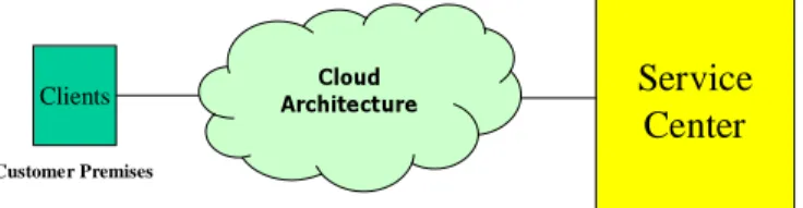
As stated in [21] and [22], the majority of current cloud computing infrastructure as of 2009 consist of services that are offered up and delivered through a service center such as a data center that can be accessed from a web browser anywhere in the world. In this paper, we study a computer service performance model for the cloud infrastructure as shown in Figure 1. This model consists of a cloud architecture (or simply called a cloud) anda service centersuch as a data center. The cloud, then in this model, isa single point of accessfor the computing needs of the customers being serviced [22] through a Web browser supported bya Web server. The service center is a collection of service resources used by a service provider to host service applications for customers, as shown in Figure 1. A service request sent by a user is transmitted to the Web server and the service center that are owned by the service provider over network [14]. As discussed before, a service application running in such a computing environment is associated with an SLA since a customer pays only for used resources and services.
The service load in cloud computing is dynamically changed upon end-users’ service requests. That is, the customer in the preceding discussion may represent
Cloud Architecture Service Center Service provider Clients Customer Premises
Fig. 1. A Computer Service Scenario in Cloud Computing
multiple users, and generates service requests at a given rate to be processed at the service center hosted by the service provider through the cloud. according to QoS requirements and for a given fee. Clearly, a customer is in general concerned about response time ranter than throughput in QoS requirements. So, we do not include throughput as a metric in this study. Other metrics may be defined in an SLA as well, but they are beyond the scope of our study in this paper.
Existing work addressing QoS requirements in com-puter service performance usually uses the average response time (or average execution time). Though the average response time is relatively easy to calculate, it does not address the concerns of a customer. Typically, a customer is more inclined to request a statistical bound on its response time than an average response time. For instance, a customer can request that 95% of the time its response time should be less than a given value. Therefore, in this paper we are concerned with a percentile of the response time that characterizes the statistical response time. That is, the time to execute a service request is less than a pre-defined value with a certain percentage of time. The metric has been used by IBM’s researchers [11] as well as it has also been called a percentile delay by scientists at Cisco [6] and MIT Communications Future Program [13]. It has been defined as the p-percentile in the standards IETF RFC5166 and RFC 2679 as well as MEF 10.1 [12]. Siripongwutikorn [18] has shown the difference of an average delay and percentile delay in per-flow network traffic analysis. By considering this percentile of response time metric, we study the relationship among the maximal number of customers, the minimal service resources and the highest level of services. We will specifically discuss the following
three important but challenging questionsfor customer service performance in cloud computing:
1) For a given arrival rate of service requests and given service rates at the Web server and the service center, what level of QoS services can
be guaranteed?
2) What are minimal service rates required at the the Web server and the service center respectively so that a given percentile of the response time can be guaranteed for a given service arrival rate from customers?
3) How many number of customers can be sup-ported so that a given percentile of the response time can be still guaranteed when service rates are given at the Web server and the service center respectively?
The problem of computer service performance mod-eling subject to QoS metrics such as response time, throughput, network utilization, have been extensively studied in the literature, for example, see [8], [10], [15], [16], and [19]. Slothouber [19] presented a model of Web server performance in which an open queueing network was employed to model the behavior of Web servers on the Internet. In [8], Karlapudi and Martin proposed and validated a Web application performance tool for the performance prediction of Web appli-cations between specified end-points. Lu and Wang [10] provided a performance model for performance analysis of NP-based Web switches. In [15], Mei and Meeuwissen recently modeled end-to-end quality of services for transaction-based services in multi-domain environments. They used the Mean Opinion Score (MOS) as a metric that is expressed by the response time and download time. In [16], Mei, Meeuwissen and Phillipson addressed the problem of an end-to-end QoS guarantee for VoIP services. The QoS metrics can be estimated by using measurement techniques [1], [2], [7], [14] and [20] as well. For example, Martin and Nilsson [14] measured the average response time of a service request. But, measurement techniques are hard to be used in computer service performance prediction. In order to compute a percentile of the response time one has to first find the probability distribution of the response time. This is not an easy task in a complex computing environment involving many com-puting nodes. Walrand and Varaiya [23] showed that in any open Jackson network, the response times of a customer at the various nodes of overtake-free path are all mutually independent. Daduna [5] further proved that the same result is valid for overtake-free paths in Gordon-Newell networks. In the paper we derive an approximation method for the calculation of the proba-bility and cumulative distributions of the response time, and show the accuracy of the proposed approximation method. Based on the obtained percentile response
time (or the cumulative distribution of response time), we derive propositions and corollaries to answer the aforementioned service performance questions in cloud computing.
The rest of the paper is organized as follows. In Section II we define the percentile of the response time and provide an example for better understanding of the definition. Then we give an approximation method for the calculation of the probability and cumulative distributions of the response time for the computer service performance model under study in Section III. A numerical validation is given in Section IV that demonstrates the accuracy of this method. Section V concludes our discussion.
II. THEPERCENTILE OFRESPONSETIME An SLA is a contract between a customer and a service provider that defines all aspects of the service that is to be provided. An SLA generally uses response time as one performance metric.
As discussed in Section I, in this paper we are interested in the percentile of the response time. This is the time it takes for a job to be executed in a computing environment consisting of multiple computing nodes.
Assume that fT(t) be the probability distribution
function of a response time T. TD is a desired target
response time that a customer requests and agrees with its service provider based on a fee paid by the customer. The SLA performance metric that a γ% SLA service is guaranteed is as follows.
Z TD
0 fT(t)dt≥γ% (1)
That is, γ% of the time a customer will receive its service in less thanTD.
As an example let us consider an M/M/1 queue with an arrival rate λand a service rate µ. The service discipline is FIFO. The steady-state probability of the system isp0 = 1−ρ,andpk= (1−ρ)ρk, k >0, where
ρ = λµ. According to Bolch et al. [4] and Perros [17], the response time T is exponentially distributed with the parameter µ(1−ρ), i.e., its probability distribution function is given by fT(t) =µ(1−ρ)e−µ(1−ρ)t.
Using the definition given in (1), we have that Z TD 0 fT(t)dt= 1−e−µ(1−ρ)TD ≥γ% (2) or µ≥ −ln (1−γ%) TD +λ (3) TABLE I
THECUMULATIVEDISTRIBUTIONFUNCTION(CDF)OFTHE
RESPONSETIME Service Rate 100 120 140 150 CDF 0.0000 0.6321 0.8647 0.9179 Service Rate 160 170 180 200 CDF 0.9502 0.9698 0.9817 0.9933 Service Rate 220 240 280 300 CDF 0.9975 0.9991 0.9999 1.0000
This means that in order to guarantee higher SLA ser-vice levels,µincreases when TD decreases. Similarly, for any given arrival rateλand service rate µ, we can use (2) to find the percentile ofγ. For example, when
λ= 100 and TD = 0.05, Table I gives the numerical values for the cumulative distribution of the response time. From this table we see that this service rate has to be bigger than 150 in order that 90% of the response time is less than 0.05.
III. A COMPUTERSERVICEPERFORMANCEMODEL As discussed before, the calculation of the percentile of response time plays a key role in answering the aforementioned performance questions. In this section, we derive the calculation.
A. The Response Time Distribution
Modeling the customer service requests as a queue-ing network model appears one of the best ways that makes it possible to not only compute percentile response time but also characterize a variable load in cloud computing. The cloud computing service model shown in Figure 1 is modeled as a queueing network model as depicted in Figure 2, which consists of a Web server and a service center. Both the Web server and the service center may have several components. But, each can be viewed as an integral element that is modeled as a single queue. External arrivals to the computing station are distributed with a rateλ. Letµi
(i = 1,2) be the service rates at the first and second queues respectively. Upon completion of a service at the service center, the customer exits the system with probability 1− β, or continues to be served at the Web server with probability β. Furthermore, after a customer is processed at the Web server, it returns to the beginning of the cloud computing system with probability1−α, or it exits the system with probability
Customer service arrivals λ Web Server µ1 T1 Service Center T2 µ2 exit b 1-b 1-a a
Fig. 2. A Queueing Performance Model for Computer Services in Cloud Computing
We are going to derive the Laplace-Stieltjes trans-form (LST) (simply called the Laplace transtrans-form al-ternatively) of response time below. Let (i, j) be the number of visits in the Web server and the service center whereiandjare the number of visits in the Web server and the number of visits in the service center respectively. Letp(i, j) be the probability of ivisits to the Web server andjvisits to the service center. There may be one time visit difference between the Web server and the service center. This means that either
j=i, orj=i−1. LetT1(λ, µ1, µ2)(orT2(λ, µ1, µ2)) be the waiting time, that is, the time from the moment a customer arrives at the Web server (or the service center) to the moment it leaves the Web server(or the service center). For notational simplicity,T1(λ, µ1, µ2)
andT2(λ, µ1, µ2) are written asT1 andT2. We further assume thatT1andT2are the same for each visit. Then, we have
#Visits Response Time Probability (1, 0) T1 p(1,0) = 1−β (1, 1) T1+T2 p(1,1) =βα (2, 1) (T1+T2) +T1 p(2,1) =β(1−α) ×(1−β) (2, 2) 2(T1+T2) p(2,2) =β2(1−α) ×α · · · · · · · · ·
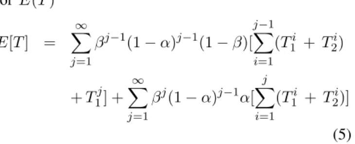
Therefore, the average response time E(T) is a weighted sum of individual response times
E[T] = ∞ X j=1 βj−1(1−α)j−1(1−β)× [(j−1)(T1 + T2) + T1] + ∞ X j=1 βj(1−α)j−1α[j(T1 + T2)] (4) Now, let Ti
1 and T2i be the response time at the
Web server and the service center for the i-th visit respectively. Then we have the following expression
for E(T) E[T] = ∞ X j=1 βj−1(1−α)j−1(1−β)[ j−1 X i=1 (T1i + T2i) +T1j] + ∞ X j=1 βj(1−α)j−1α[ j X i=1 (T1i + T2i)] (5) Let R(j, j−1)be the response time for j visits to
T1 and j−1 visits toT2, and R(j, j) be the response
time for j visits to T1 andT2. Then
R(j, j −1) = j−1 X i=1 (T1i + T2i) + T1j R(j, j) = j X i=1 (T1i + T2i) (6) Assume that Ti
1 and T1k, T2i and T2k, and T1i and Ti
2 are mutually independent (i6= k). Under these
as-sumptions, the conditional Laplace-Stieltjes transforms (LSTs) of the response timesR(j, j−1) andR(j, j)
can be expressed as follows.
LR(j, j−1)(s) = (LT1(s)) j×(L T2(s)) j−1 LR(j, j)(s) = (LT1(s)) j×(L T2(s)) j (7)
By combining equation (5) with (7), we obtain the LST of the total response time:
LT(s) = ∞ X j=1 βj−1(1−α)j−1(1−β)LjT 1(s)L j−1 T2 (s) + ∞ X j=1 βj(1−α)j−1αLjT 1(s)L j T2(s) That is, LT(s) = (1−1β−)Lβ(1T1(−s) +α)LαβLT1(s)LT2(s) T1(s)LT2(s) (8) We can further get the cumulative distribution of re-sponse time by inverting the Laplace transform of (8):
FT(t, λ, µ1, µ2) =L−1{LT(s)/s} (9)
where L−1 is an invert Laplace transform. Generally
speaking, there is no closed-form solution for the version of the above Laplace transform. Hence, the in-version is usually done numerically. Thus, the answers to the aforementioned first two questions in Section I can be expressed by the following corresponding two propositions.
Proposition 1: For a given arrival rate λ, service ratesµ1in the Web server andµ2 in the service center,
and a set of parameters α, β, and TD, the level of
QoS guaranteed services (γ) will be no more than
100FT(TD, λ, µ1, µ2).
Proof.This is because the percentile of response time is equal to 1−FT(TD, λ, µ1, µ2). By a use of this, it
easy to derive this proposition.
Proposition 2: For a given arrival rate λ, a level of QoS servicesγ, and a set of parametersα, β, andTD, service rate µ1 in the Web server and service rate µ2
in the service center are determined by solving forµ1
andµ2 in the optimization problem below:
argminµ
1∈R1, µ2∈R2
³
FT(TD, λ, µ1, µ2)−1´
subject toFT(TD, λ, µ1, µ2)≥γ%, where R1 andR2
are sets of all permission values for service rates µ1
and µ2 respectively. For example, R1 = R2 = R+
which is a set of positive real numbers, i.e., a positive real line.
Furthermore, assume that there arencustomers, each with an equivalent arrival rate of λ0. Let λ = nλ0. Then, an answer to the third question raised in Section I can be expressed by the following proposition.
Proposition 3: For service rates µ1 and µ2, a level
of QoS services γ, and a set of parameters α, β, and
TD, the maximal number of customers that can be
supported without a violation of a predefined level of QoS servicesγ%is determined by solving fornin the integer optimization problem below:
argmaxn∈I³FT(TD, nλ0, µ1, µ2)−1
´
subject to FT(TD, nλ0, µ1, µ2) ≥γ%, where I+ is a
set of all permission values for the number of customers
n. For example,I+ is a set of all positive integers.
Similar to the proof of Propositions 1, we can easily prove Propositions 2 and 3. They are omitted due to the page limit.
We see that FT(TD, λ, µ1, µ2) will play a key role
in Propositions 1-3 in answers to the three questions of Section I. As stated before, its expression can be numerically found.
Next, an interesting case is considered below in which the closed-form expression ofFT(TD, λ, µ
1, µ2)
is derived.
Assume that the Web server and the service center are each modeled as an M/M/1 queue. The service discipline is FIFO. External arrivals to the computing station are Poisson distributed and the service times at the Web server and the service center are exponentially distributed. Let λi (i = 1,2) be the arrival rates at
the first and secondM/M/1queues respectively. Then,
traffic equations are given byλ1=λ+ (1−α)λ2 and λ2 = βλ1. Thus, the following expressions of λ1 and λ2 can be derived from these local balance equations: λ1 = 1−(1λ−α)β andλ2 = 1−(1λβ−α)β.
Moreover, the LSTs of the response time at each queue isLT1(s) = a1 s+a1,where a1 =µ1(1−ρ1), ρ1= λ1 µ1andLT2(s) = a2 s+a2,wherea2 =µ2(1−ρ2), ρ2 = λ2 µ2.
It follows from (8) that
LT(s) = (sa+1(1a −β)(s+a2) +a1a2αβ
1)(s+a2)−a1a2β(1−α) (10)
whose de-numerator is a quadratic polynomial with respect to variable s that has the roots
s1,2 = −(a1+a2)±
p
(a1+a2)2−4a1a2(1−β+αβ)
2
(11) Notice that both α andβ range from 0 to 1. Hence,
1−β+αβ is non-negative. This means thats1 ands2
must be non-positive, and eithers1 ors2 is zero if and only if1−β+αβ= 1−β(1−α) = 0, i.e.,α =β= 1, which is a less interesting case.
Moreover, from (10) we can have that
LT(s) = a1(1−β()ss−+sa1a2(1−β+αβ) 1)(s−s2) 4 = B1 s−s1 + B2 s−s2 (12)
where constants B1 andB2 are given by
(
B1 = a1s1(1−β)+a1a2(1−β+αβ)
s1−s2
B2 =−a1s2(1−β)+s1a−1as2(12 −β+αβ)
(13)
Therefore it follows from (12) that the probability distribution function of response timeT is
fT(t) =B1es1t+B
2es2t (14)
The closed-form expression ofFT(t, λ, µ1, µ2))is thus
given by FT(t, λ, µ1, µ2)) = 1 + µ B1 s1 e s1TD+ B2 s2 e s2TD 
To ensure thatγ%of the response time for customer service requests are not more than a desired target response time TD, we require that G(TD) = 1 −
FT(t, λ, µ1, µ2))≤1−γ%. That is, µ B1 s1 e s1TD +B2 s2 e s2TD ¶ ≥γ%−1 (15) From equation (15) and Proposition 1, we can first determine the service level (=γ%) for a given arrival rate and given service rates. That is, we have the
following corollary for answering Question 1 presented in Section I.
Corollary 1: The level of QoS guaranteed services (γ) will be no more than
100 · 1 + µ B1 s1 e s1TD +B2 s2 e s2TD ¶¸
Second, from equation (15) and Proposition 2, we can find service rates necessary to ensure a certain service level as in (2) and (3). It can be shown that
G(TD)is a decreasing function with respect to service
rates µ1 andµ2. Hence, more specifically, Proposition
2 can be rewritten as follows.
Corollary 2: Service rate µ1 in the Web server and
service rate µ2 in the service center are the solution of
an optimization problem below: argminµ1∈R1, µ2∈R2 µ B1 s1 e s1TD +B2 s2 e s2TD ¶ subject toγ%≤1+³B1 s1 e s1TD +B2 s2 e s2TD ´ , wheres1, s2, B1, andB2 are given in (11) and (13).
Finally, Proposition 3 is reduced as follows.
Corollary 3: The maximal number of customers that can be supported without a violation of a predefined level of QoS services γ%is the solution of an integer optimization problem below:
argmaxn∈I µ B1 s1 e s1TD+ B2 s2 e s2TD ¶ subject to γ%≤1 +³B1 s1 e s1TD +B2 s2 e s2TD ´ .
The constrained optimization problems are two- and one- dimensional, which can be easily solved by using existing numerical tools (e.g., Matlab).
IV. A NUMERICALVALIDATION
In this section we validate the correctness of Propo-sitions 1-3 and Corollaries 1-3 and demonstrate how to find answers to the three questions given in Section I. Since the expression of percentile response time is usually not a closed form and it is required to find the solutions of optimization problems in Propositions 2-3 and Corollaries 2-3, the correctness of these proposi-tions and corollaries can be only validated numerically by a comparison of model simulation results. That is, the way to find the answers to three questions in Section I is a numerical approximate method. The relative error % is used to measure the accuracy of the approximate results compared to model simula-tion results, and it is defined by Relative error % =
Approximate Result−Simulation Result
Simulation Result × 100. We
study the accuracy of our proposed approximation method using an example below.
We shall verify the accuracy of the approximate method for the computing system analyzed in Section III. We let λ= 100, µ1 = 380, µ2 = 200, and α and β were varied.
We simulated the queueing network using Arena (see [3]), and the analytical method was implemented in Matlab and also in Mathematica. The simulation model in Arena exactly represents the computer service per-formance model under study, so the simulation results in Arena are considered as “exact”.
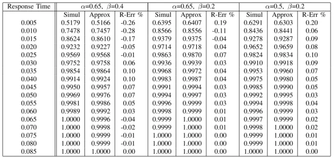
Table II presented on next page shows the simulated and approximate cumulative distribution function of the response time for different values of α and β. In the table, columns labeled “Simul” gives the simulation result, columns labeled “Approx” gives the approximate result, and columns labeled “R-Err %” gives their relative errors. Those abbreviations are also used in other tables of this section. It appears that the results obtained by our approximate method are fairly good.
For example, when α = 0.5, β = 0.2, both results reflects that98% of time the customer requests will be responded in less thanTD = 0.025 as shown in Table
II. This means that when λ = 380, µ1 = µ2 = 200, α = 0.5, β = 0.2, and TD = 0.025, the level of QoS
services γ%is no less than 98%.
Second, both Propositions 2 and 3 (or Corollaries 2 and 3) require us to solve an optimization problem. In order to get service rates µ1 and µ2 for a given
arrival rate λ, we are required to find a solution of the two-dimensional optimization problem given in Proposition 2 (or Corollary 2). Meanwhile, in order to get the maximal number of customers n for given service rates µ1 and µ2, we are required to find a
solution of the integer optimization problem given in Proposition 3 (or Corollary 3). Generally speaking, an integer optimization problem is more difficult to solve than a two-dimensional optimization problem whose parameters can be chosen as real positive numbers. Hence, in the following simulation we only consider Proposition 3 (or Corollary 3) to demonstrate how to find a solution of the integer optimization problem. Thus, the numerical example for Proposition 2 (or Corollary 2) is omitted in this paper due to the page limit. Letλ0= 10,µ1 = 400,µ2= 250,α= 0.6,β = 0.4, TD = 0.02, and γ% = 94.5. Then, λ 1 and λ2 are calculated by λ1 = 1−0.λ4×0.4 = 0.084n ≈ 11.905 and λ2 =λ1β = 0.n21 ≈4.762n.
TABLE II
THECUMULATIVEDISTRIBUTIONFUNCTIONS OFTHERESPONSETIME
Response Time α=0.65, β=0.4 α=0.65, β=0.2 α=0.5, β=0.2 Simul Approx R-Err % Simul Approx R-Err % Simul Approx R-Err % 0.005 0.5179 0.5166 -0.26 0.6395 0.6407 0.19 0.6291 0.6303 0.20 0.010 0.7478 0.7457 -0.28 0.8566 0.8556 -0.11 0.8436 0.8441 0.06 0.015 0.8624 0.8610 -0.17 0.9379 0.9375 -0.04 0.9278 0.9287 0.09 0.020 0.9232 0.9227 -0.05 0.9714 0.9718 0.04 0.9652 0.9659 0.08 0.025 0.9569 0.9568 -0.01 0.9863 0.9870 0.07 0.9824 0.9834 0.10 0.030 0.9752 0.9758 0.06 0.9936 0.9939 0.03 0.9910 0.9918 0.09 0.035 0.9854 0.9864 0.10 0.9968 0.9972 0.04 0.9953 0.9960 0.07 0.040 0.9914 0.9924 0.10 0.9983 0.9987 0.04 0.9975 0.9980 0.05 0.045 0.9950 0.9957 0.07 0.9991 0.9994 0.03 0.9985 0.9990 0.05 0.050 0.9969 0.9976 0.07 0.9994 0.9997 0.03 0.9992 0.9995 0.03 0.055 0.9981 0.9986 0.05 0.9996 0.9999 0.03 0.9994 0.9998 0.04 0.060 0.9989 0.9992 0.03 0.9998 0.9999 0.01 0.9996 0.9999 0.03 0.065 1.0000 0.9996 -0.04 0.9999 1.0000 0.01 0.9997 0.9999 0.02 0.070 1.0000 0.9998 -0.02 0.9999 1.0000 0.01 0.9998 1.0000 0.02 0.075 1.0000 0.9999 -0.01 1.0000 1.0000 0.00 0.9999 1.0000 0.01 0.080 1.0000 0.9999 -0.01 1.0000 1.0000 0.00 0.9999 1.0000 0.01 0.085 1.0000 1.0000 0.00 1.0000 1.0000 0.00 1.0000 1.0000 0.00
Furthermore, it follows from (11) that
s1,2=
©
−(650−16.666n)±£(650−16.666n)2−
3.36(400−11.905n)(250−4.762n)]}/2
(16) and from (13) we can obtain expressions ofB1andB2.
Then, by using either existing numerical tools (e.g., Mathematica, Matlab or Maple) or developing our own numerical tool, we can solve for n in the integer optimization problem presented in Proposition 3 (or Corollary 3). In the numerical implementation, we obtainn= 9. This means that at most 9 customers can be supported so that 94.5% of time all 9 customers’ requests can be completed in 0.02. We also simulated the computer service model and validated using the brute-force approach that n = 9 by using the closed-form solution is actually optimal. Table III gives the cumulative distribution of the response time obtained using Proposition 3 (or Corollary 3) and the simulation method. We noticed that Proposition 3 (or Corollary 3) gives us a very accurate solution.
In this approximation method, we assume that the waiting time of a customer at the Web server (or the service center) is independent of the waiting times at the service center (or the cloud), and it is also independent of its waiting times in other visits to the same the Web server (or the same service center). Hence, the relative error as shown in Table II is due to the above assumptions.
TABLE III
THECUMULATIVEDISTRIBUTIONFUNCTIONS OFTHE
RESPONSETIME
Response Time Simul Approx R-Err% 0.005 0.5595 0.5594 -0.0258 0.010 0.7924 0.7954 0.3786 0.015 0.8996 0.8997 0.0092 0.020 0.9510 0.9495 -0.1598 0.025 0.9760 0.9741 -0.1973 0.030 0.9883 0.9861 -0.2179 0.035 0.9942 0.9933 -0.0947 0.040 0.9972 0.9963 -0.0880 0.045 0.9986 0.9980 -0.0617 0.050 0.9993 0.9989 -0.0422 0.055 0.9997 0.9994 -0.0267 0.060 0.9998 0.9996 -0.0237 0.065 0.9999 0.9998 -0.0120 0.070 1.0000 0.9998 -0.0161 0.075 1.0000 0.9999 -0.0081 0.080 1.0000 0.9999 -0.0091 V. CONCLUSIONS
We have studied three important but challenging questions for computer service performance in cloud computing below: (1) For given service resources, what level of QoS services can be guaranteed? (2) For a given number of customers, how many service resources are required to ensure that customer services can be guaranteed in term of the percentile of re-sponse time? (3) For given service resources, how many customers can be supported to ensure that customer services can be guaranteed in term of the percentile of
response time?
The main difficulty for answering these three ques-tions to understand the characteristics of computer ser-vice performance is in the computation of the probabil-ity distribution function of response time. In this paper, we have first proposed a queueing network model for studying the performance of computer services in cloud computing, and then developed an approxima-tion method for computing the Laplace transform of a response time distribution in the cloud computing system. Therefore, we have derived three propositions and three corollaries for answering the above three questions. The answers to the above three questions can be obtained by using a numerical approximate method in these propositions and corollaries.
We have further conducted numerical experiments to validate our approximate method. Numerical results showed the the proposed approximate method provided a good accuracy for the calculation of cumulative distri-butions of the response time, and the maximal number of customers for given computer service resources in cloud computing in which customer services can be guaranteed in the term of the percentile of response time. Hence, the proposed method provides an efficient and accurate solution for the calculation of probability and cumulative distributions of a customer’s response time. It will be useful in the services performance prediction of cloud computing. We plan to apply our proposed method to test cloud computing infrastructure once it is available to us for a real-world test. Addition-ally, the Web server and the service center have been modeled as a infinite queue for single-class customers in this paper. The methods given in [25] and [26] can be applied to discuss a finite queue for single- and multiple-class customers, which will be presented in another paper.
REFERENCES
[1] J. Aikat, J. Kaur, F. Smith, and K. Jeffay, “Variability in TCP round-trip times”, In Proceedings of the ACM SIGCOMM Internet Measurement Conference, October, 2003.
[2] M. Allman, W. Eddy, and S. Ostermann, “Estimating loss rates with TCP,”ACM Performance Evaluation Review, 31(3), December, 2003.
[3] T. Altiok and B. Melamed,Simulation Modeling and Analysis with Arena, Cyber Research, Inc. 2001.
[4] G. Bolch, S. Greiner, H. Meer, and K. Trivedi, Queueing
Networks and Markov Chains,” Hohn Wiely and Sons, New
year, 1998.
[5] H. Daduna, “Burke’s theorem on passage times in Gordon-Newell networks,” Adv. Appl. Prob., 16, 1984.
[6] B. Davie, “Interprovider QoS” 2004.
[7] K. Gummadi, S. Saroiu, and S. Gribble “King: Estimating latency between arbitrary Internet end hosts,” InProceedings
of the ACM SIGCOMM Internet Measurement Workshop,
November, 2002.
[8] H. Karlapudi, and J. Martin “Web application performance prediction,” InProceedings of the IASTED International Con-ference on Communication and Computer Networks, pp. 281-286, Boston, MA, Nov 2004.
[9] W. Kim, “‘Cloud computing: Today and Tomorrow,”Journal of Object Technology, 8, 2009.
[10] J. Lu, and J. Wang, “Performance modeling and analysis of Web Switch,” InProceedings of the 31st Annual International
Conference on Computer Measurement (CMG05), Orlando,
FL, Dec 2005.
[11] C. Matthys, et al.,On Demand Operating Environment: Man-aging the Infrastructure (Virtualization Engine Update),” IBM Redbooks, June, 2005.
[12] MEF 10.1, “Ethernet Service Attributes Phase 2,” November 2006.
[13] MIT Communications Future Program, “Inter-provider Qual-ity of Service,” 2006.
[14] J. Martin, and A. Nilsson, “On service level agreements for IP networks,” InProceedings of the IEEE INFOCOM, June 2002.
[15] R. D. Mei, H. B. Meeuwissen, and F. Phillipson, “User perceived Quality-of-Service for voice-over-IP in a heteroge-neous multi-domain network environment,” InProceedings of ICWS, Sept 2006.
[16] R. D. Mei, and H. B. Meeuwissen, “Modelling end-to-end Quality-of-Service for transaction-based services in multi-domain environement,” In Performance Challenges for Ef-ficient Next Generation Networks (Eds. X. J. Liang, Z. H. Xin, V. B. Iversen and G. S. Kuo), Proceedings of the 19th International Teletraffic Congress (ITC19), pp. 1109-1121, Beijing, China, Aug 2005.
[17] H. Perros, Queueing Network with Blocking, Exact and Approximate Solutions, Oxford University Press, 1994. [18] P. Siripogwutikorn and S. Banerjee, “Per-flow delay
perfor-mance in traffic aggregates,” In Proceedings of the IEEE
GLOBECOM,2006.
[19] L. Slothouber, “A model of Web server performance,” www.geocities.com/webserverperformance, 1995.
[20] J. Sommers, P. Barford, N. Duffield, and A. Ron, “Improving accuracy in end-to-end packet loss measurement,” In
Pro-ceedings of the ACM SIGCOMM, August, 2005.
[21] Wikipedia, “Cloud Computing,” In http://en. wikipedia.org/wiki/Cloud_computing.
[22] Tech, “What is Cloud Computing,” In
http://jobsearchtech.about.com/od/ historyoftechindustry/a/cloud_computing. htm.
[23] J. Walrand and P. Varaiya, “Sojourn times and the overtaking condition in Jacksonian networks,”Adv. Appl. Prob., 12, 1980. [24] L. Vaquero and L. Rodero-Merino and J. Caceres and m. Lindner, “A break in the clouds: towards a cloud definition,”
ACM SIGCOMM Computer Communication Review, vol. 39,
no.1, 2009.
[25] K. Xiong and H. Perros, “Computer resource optimization for differential customer services,” InProceedings of the 14th
IEEE MASCOTS, 2006.
[26] K. Xiong and H. Perros, “SLA-based resource allocation in cluster computing systems,” In Proceedings of the IEEE IPDPS, 2008.