Applications of Machine Learning: From Single Cell Biology to Algorithmic Fairness

(1)

Applications of Machine Learning: From Single Cell Biology to Algorithmic

Fairness

by

Alexander H. S. Vargo

A dissertation submitted in partial fulfillment of the requirements for the degree of

Doctor of Philosophy (Mathematics)

in the University of Michigan 2020

Doctoral Committee:

Professor Anna C. Gilbert, Chair Professor Daniel Burns

Professor Jun Z. Li

Associate Professor Indika Rajapakse Assistant Professor Yuekai Sun

(2)

Alexander H. S. Vargo [email protected] ORCID iD: 0000-0001-5930-8841

(3)

Dedication

(4)

Acknowledgments

First and foremost, I extend my deep gratitude to Anna Gilbert, my advisor. This dissertation would not have been possible without Anna’s support, patience, and mathematical insight. Her guidance and perspective have illuminated my path from pupil to researcher.

Thanks also to Jun Li, who helped me understand the benefits of interdisciplinary collaboration. Jun’s wisdom and anecdotes make research questions transcend any professional languages, and his constant questioning has assisted the development of my critical eye. I further greatly appreciate the collaboration of the other members of the Michigan Center for Single-Cell Genomic Data Analytics; our meetings and conversations were a highlight of my graduate experience.

In addition, many thanks to Yuekai Sun. Yuekai is always down to earth and relatable, but produces interesting observations at a shocking pace. He fueled my interest in algorithmic fairness, and is always open to working on another project. Thanks also to my other algorithmic fairness collaborators Martin Strauss, Suresh Venkatasubramanian, Laura Niss, Amanda Bower, and Fan Zhang. Special thanks to Laura and Amanda: our discussions together have resulted in some of the most productive and important insights of my career.

I am additionally grateful to the many others who have acted as advisors and mentors throughout my academic life. Thanks to my other committee members Daniel Burns and Indika Rajapakse. Special thanks to Karen Smith: I benefited from her mathematical prowess as her student early in my graduate experience, and she has consistently pushed and supported me since then. Also thanks to Anne Speigle and Teresa Stokes; without their help, this project would not have been completed.

Furthermore, thanks to my fellow graduate students and friends. Your discussions have consis-tently lightened my mood, and I am looking forward to seeing your future success. Notably, Umang Varma and I forged a similar path through academia, and I value his wisdom and friendship. Finally, a massive thank you to my parents and my brother. Their confidence in my abilities, even in my most difficult times, has propelled me to where I am today.

This research was supported in part through computational resources and services provided by Advanced Research Computing at the University of Michigan, Ann Arbor. Funding was provided in part by the University of Michigan Department of Mathematics, the Michigan Institute for Data Science, and the Chan Zuckerberg Initiative.

(5)

LIST OF FIGURES

FIGURE

2.1 Counts of gene PRTN3 in bone marrow cells in the PAULdata set (See ). Each point corresponds to a cell; the horizontal axis shows the number of reads and the vertical axis shows the number of cells with a fixed number of reads. No library size or cell size normalization has been carried out in these pictures. Note that the tail of the log transformed data is subjectively longer, while the gap between zero counts and nonzero counts appears larger in the rank transformed data . . . 16 2.2 A visual description of 5 fold cross-validation . . . 26 2.3 Performance of the marker selection methods on the (a) ZEISEL, (b) PAUL, and (c)

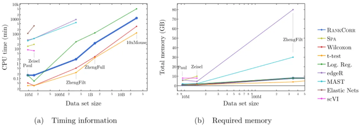
ZHENGFILT data sets as the number of selected markers is varied. There are two rows for each method; the first row for each method represents the classification metrics and the second row represents the clustering metrics. Blue indicates better performance than the other methods; orange indicates notably worse performance than the other methods. The marker bins are chosen to emphasize certain features in Figures 2.5-2.11; these figures present the values of the evaluation metrics for the different data sets. The values in the boxes correspond to a ranking of the methods, with 1 being the best method in the marker range. The classification and clustering results are ranked separately. Further notes: (a) All of the methods perform well on the ZEISEL data set - an orange box here does not indicate poor performance, but rather that other methods outperformed the orange one. (b) Many of the methods showed nearly identical performance according to the classification metrics; thus, this table contains many yellow boxes. . . 37 2.4 Computational resources used by the marker selection methods. In both figures, the

data set size is the number of entries in the data matrixX: it is given byn×p, the number of cells times the number of genes. The sizes of the data sets that we consider in this work are indicated in the figures. The total CPU time required to select markers on one fold in the experimental data sets is shown in (a); the total memory required during these trials is shown in (b). Elastic nets scales poorly in (a), so it is only run on PAULand ZEISEL. Both edgeR and MAST are limited by memory on ZHENGFILT(see (b)); this prevents their application to the larger data sets. scVI also requires a GPU while it is running; this prevents us from testing it on the larger data sets. RANKCORR, the t-test, Wilcoxon, and logistic regression all use 8 GB to run on ZHENGFULLand 80 GB to run on 10XMOUSE. See the Sectionsec:markMeth for more details. . . 38

(9)

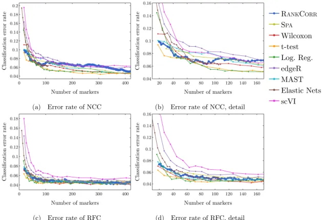
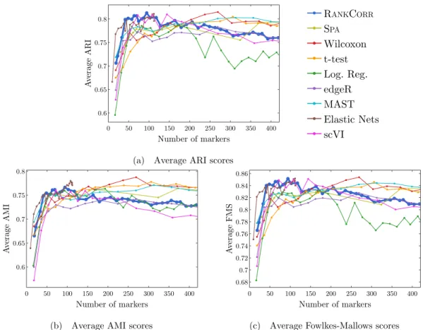
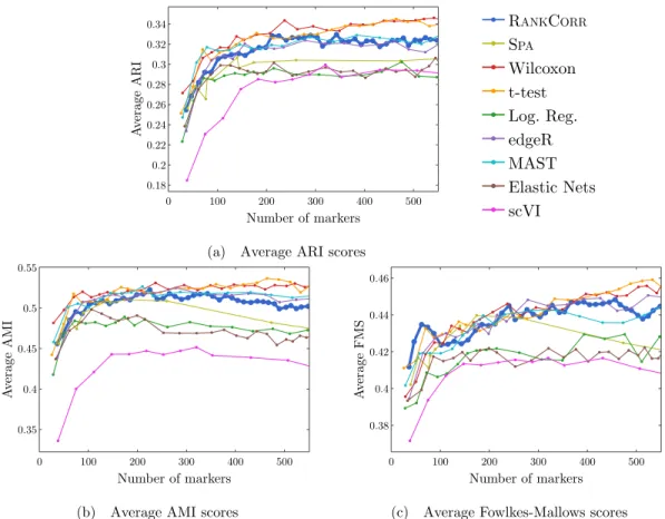
2.5 Error rate of both the nearest centroids classifier (NCC; (a) and (b)) and the random forests classifier (RFC; (c) and (d)) on the Zeisel data set. Figure (b) (respectively (d)) is a detailed image of the error rate of the different methods using the NCC (respectively RFC) when smaller numbers of markers are selected. . . 39 2.6 Clustering performance metrics vs total number of markers selected for marker

selec-tion methods on the ZEISELdata set. The ARI score is shown in (a), the AMI score is

shown in (b), and the Fowlkes-Mallows score is shown in (c). The clustering is carried out using 5-fold cross validation and scores are averaged across folds. . . 40 2.7 Error rates of both the nearest centroids classifier (NCC; (a) and (b)) and the random

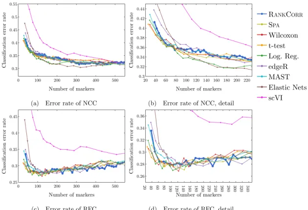
forests classifier (RFC; (c) and (d)) on the Paul data set. Figure (b) (respectively (d)) is a detailed image of the error rate of the different methods using the NCC (respectively RFC) when smaller numbers of markers are selected. Figure (b) details up to 220 total markers to make clear how similar the methods perform for when small numbers of markers are selected. Figure (d) examines up to 350 total markers to detail the performance of the methods when small numbers of markers are selected as well as get an idea for the increasing behavior and noisy nature of the curves. . . 42 2.8 Clustering performance metrics vs total number of markers selected for marker

selec-tion methods on the PAULdata set. The ARI score is shown in (a), the AMI score is

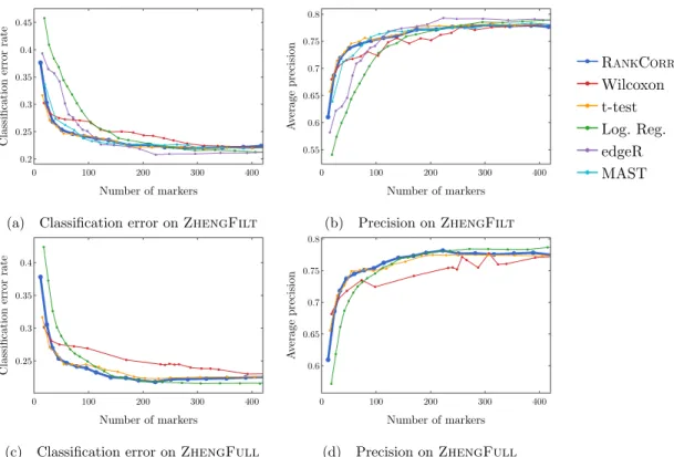
shown in (b), and the Fowlkes-Mallows score is shown in (c). The clustering is carried out using 5-fold cross validation and scores are averaged across folds. . . 43 2.9 Accuracy and precision of the nearest centroids classifier on the ZHENGdata sets using

the bulk labels. The top row correspond to the ZHENGFILT data set and the bottom row corresponds to the ZHENGFULLdata set. . . 44

2.10 Accuracy and precision of the random forests classifier on the ZHENG data sets using

the bulk labels. The top row correspond to the ZHENGFILT data set and the bottom row corresponds to the ZHENGFULLdata set. . . 45

2.11 Clustering metrics on the ZHENGFILTdata set. . . 46

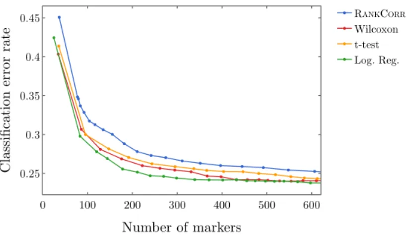
2.12 Classification error rate under the NCC vs number of markers on the full 10XMOUSE

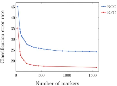
data set. . . 48 2.13 A comparison of the nearest centroid classifier (NCC) and the random forest classifier

(RFC) using the RANKCORRmethod on the 10XMOUSEdata set . . . 49 2.14 Set up of the simulated data. We consider 3 conditions: all genes used for simulation,

filtering after simulation, and filtering before simulation. On the left side of this diagramme, we produce 10 data sets by using all genes in simulation, and 10 more by filtering down to the 5000 most variable genes after simulation. These “filtering after simulation” data sets contain a subset of the information from the “all genes used for simulation” data sets. On the right hand side, we produce 10 data sets by filtering down to the 5000 most variable before simulation. . . 51 2.15 Precision of the marker selection methods versus the number of markers selected for

the first 400 markers selected. Each sub-figure corresponds to a simulation method and the four lines correspond to the different marker selection algorithms. The RANKCORR

method consistently shows the highest precision across all three simulation methods. . 52 2.16 ROC curves. Each sub-figure corresponds to a simulation method and the four lines

correspond to the different marker selection algorithms. The solid (purple) line is the diagonal TPR = FPR. . . 53

(10)

2.17 Clustering error rates using the Random Forest classifier for the first 500 markers chosen by each method. The sub-figures correspond to different simulation conditions. The RANKCORRalgorithm consistently produces the smallest values of the clustering

error rate. . . 55

3.1 Rank space in 3 dimensions. See the text for further description . . . 80

4.1 The model (4.1) and (4.2). . . 105

4.2 . . . 110

4.3 Distribution of recidivism probabilities from raw and debiased representations for African-Americans. . . 110

5.1 Comparison of GBDT classifiers without (a) and with (b) the fairness constraints introduced in this paper. The classifiers output a probability in[0,1]- these probabilities are discretized to binary labels to create a classification. In the figures, red points are individuals with true label 0 and blue points are individuals with true label 1. The darker red areas correspond to lower output probabilities and the darker blue areas correspond to higher output probabilities. The arrows in (b) indicate the transport map corresponding to the fairness constraint for the previous boosting step. . . 134

5.2 Fairness measures at given accuracy levels for the BuDRO method on the Adult data set, considered over 10 train/test splits. The results from each choice of hyperparameters are averaged over all train/test splits before being grouped into accuracy bins. The plotted points are the ones from each bin that optimize the specified quantity ((a) averageGap_RMS, (b) raceGap_RMS, (c) genderGap_RMS, (d) spouse consistency). Error bars represent one standard deviation. Empirically, the gender gaps were harder to reduce than the race gaps. The S-cons in all of these pictures never drops below 94%. . 145

5.3 The accuracy vs fairness trade-off of BuDRO when compared to other baseline boosting algorithms on the Adult data set. All lines are chosen to minimize genderGap_RMS. (a) contains a comparison of the Gender gap RMS. The BuDRO line also appears in Figure 5.2(c). (b) contains a comparison of the S-cons. Error bars represent one standard deviation. . . 147

A.1 Supervised classification metrics for the ZEISEL data set using the nearest centroid classifier (NCC). Included is the performance of the scGeneFit method. (a) is the classification error rate including a curve corresponding to random marker selection (the curve that starts at around 50% error). (b) contains the precision and (c) contains the Matthews correlation coefficient. Data from random marker selection are not included in figures (b) and (c) for clarity. Note that the curves in (b) are similar in shape to the curves in (c); they are also similar in shape to the classification accuracy (1−classification error rate from Figure 4(a) of the main manuscript). . . 149

(11)

A.2 Supervised classification metrics for the ZEISEL data set using the random forests classifier (RFC). Included is the performance of the scGeneFit method. (a) is the classification error rate including a curve corresponding to random marker selection (the curve that starts at around 45% error). (b) contains the precision and (c) contains the Matthews correlation coefficient. Data from random marker selection are not included in figures (b) and (c) for clarity. Note that the curves in (b) are similar in shape to the curves in (c); they are also similar in shape to the classification accuracy (1−classification error rate from Figure 4(c) of the main manuscript). . . 150 A.3 Unsupervised clustering metrics for the ZEISELdata set including data from random

marker selection. The curve corresponding to random marker selection is shown in grey and is the lowest (worst) curve in all three plots. The ARI score is shown in (a), the AMI score is shown in (b), and the Fowlkes-Mallows score is shown in (c). The clustering is carried out using 5-fold cross validation and scores are averaged across folds. . . 151 A.4 Supervised classification metrics for the PAUL data set using the nearest centroid

classifier (NCC). Included is the performance of the scGeneFit method. (a) is the classification error rate including a curve corresponding to random marker selection (the curve that starts at around 75% error). (b) contains the precision and (c) contains the Matthews correlation coefficient. Data from random marker selection are not included in figures (b) and (c) for clarity. Note that the curves in (b) are similar in shape to the curves in (c); they are also similar in shape to the classification accuracy (1−classification error rate from Figure 6(a) of the main manuscript). . . 152 A.5 Supervised classification metrics for the PAUL data set using the random forests

classifier (RFC). Included is the performance of the scGeneFit method. (a) is the classification error rate including a curve corresponding to random marker selection (the curve that starts at around 65% error). (b) contains the precision and (c) contains the Matthews correlation coefficient. Data from random marker selection are not included in figures (b) and (c) for clarity. Note that the curves in (b) are similar in shape to the curves in (c); they are also similar in shape to the classification accuracy (1−classification error rate from Figure 6(c) of the main manuscript). . . 153 A.6 Unsupervised clustering metrics for the PAUL data set including data from random

marker selection. The curve corresponding to random marker selection is shown in grey and is the lowest (worst) curve in all four plots. The ARI score is shown in (a), the AMI score is shown in (b), and the Fowlkes-Mallows score is shown in (c). (d) contains the FM scores for larger numbers of markers selected, showing the scVI does approach the behavior of random marker selection in this case. Each clustering is carried out using 5-fold cross validation and scores are averaged across folds. . . 154 A.7 Supervised classification metrics for the ZHENGFILTdata set using the nearest centroid

classifier (NCC). (a) is the classification error rate including a curve corresponding to random marker selection (the curve that starts at around 90% error). (b) contains the Matthews correlation coefficient. Data from random marker selection are not included in (b). Note that (b) is similar in shape to the classification accuracy (1−classification error rate from Figure 8(a) of the main manuscript). . . 155

(12)

A.8 Supervised classification metrics for the ZHENGFILTdata set using the random forests classifier (RFC). (a) is the classification error rate including a curve corresponding to random marker selection (the curve that starts at around 70% error). (b) contains the Matthews correlation coefficient. Data from random marker selection are not included in (b). Note that (b) is similar in shape to the classification accuracy (1−classification error rate from Figure 9(a) of the main manuscript). . . 155 A.9 Supervised classification metrics for the ZHENGFULLdata set using the nearest

cen-troid classifier (NCC). (a) is the classification error rate including a curve corresponding to random marker selection (the curve that starts at around 90% error). (b) contains the Matthews correlation coefficient. Data from random marker selection are not included in (b). Note that (b) is similar in shape to the classification accuracy (1−classification error rate from Figure 8(c) of the main manuscript). . . 156 A.10 Supervised classification metrics for the ZHENGFULLdata set using the random forests

classifier (RFC). (a) is the classification error rate including a curve corresponding to random marker selection (the curve that starts at around 70% error). (b) contains the Matthews correlation coefficient. Data from random marker selection are not included in (b). Note that (b) is similar in shape to the classification accuracy (1−classification error rate from Figure 9(c) of the main manuscript). . . 156 A.11 Unsupervised clustering metrics for the ZHENGFILT data set including data from

random marker selection. The curve corresponding to random marker selection is shown in grey and is the lowest (worst) curve in all three plots. The ARI score is shown in (a), the AMI score is shown in (b), and the Fowlkes-Mallows score is shown in (c). Each clustering is carried out using 5-fold cross validation and scores are averaged across folds. . . 157 A.12 Supervised classification metrics for the 10XMOUSEdata set using the nearest centroid

classifier (NCC). (a) is the classification error rate figure found in Figure 9 of the main manuscript, for reference here. (b) contains the average precision curves and (c) contains the Matthews correlation coefficient curves. We do not compare to random markers on this data set. . . 158 A.13 The classification accuracy under the RFC on the PAULdata set (see the Methods in

the main manuscript) run twice with the same markers used for each point. Significant variation is observed in the classification accuracy over the two classification attempts. Differences of nearly 2% are observed between the two curves. . . 159 A.14 Effect of changing the number of nearest neighbors on the ARI, AMI, and FM scores

for the ZEISELdata set using RANKCORRto select markers. Clustering was performed with Louvain and the scores were optimized over the resolution. It appears that 15 nearest neighbors is too few, while 30 nearest neighbors is too many.. . . 160 A.15 Effect of changing the number of nearest neighbors on the ARI, AMI, and FM scores

for the PAUL data set using RANKCORRto select markers. Clustering was performed

with Louvain and the scores were optimized over the resolution. All of the choices of numbers of nearest neighbors produce similar curves for all three scores. Choosing 30 nearest neighbors appears to provide increased performance for small numbers of markers.. . . 161

(13)

A.16 Clustering the 68k PBMC data set from [ZTB+17] (reference [2] from the main manuscript) with Louvain clustering. (a) contains a UMAP plot of the bulk la-bels. (b) is a UMAP plot of a Louvain clustering of the data set. It was created by first filtering to the 1000 most variable genes using thecell rangerflavor of

thefilter genes dispersion function in thescanpypython package. The

Louvain algorithm was run on the top 50 PCs and used 25 nearest neighbours for each cell with a resolution parameter of 0.3. The Louvain clustering solution subjectively looks similar to the bulk labels. The ARI for the clustering compared to the bulk labels is 0.345, the AMI is 0.565, and the FMS is 0.462 (these values have been rounded to 3 significant digits).. . . 162 A.17 UMAP projection of the data consisting of ZHENGFULLcombined with the isolated

CD19+ B cell data set from [ZTB+17] (reference [2] from the main manuscript) that was used to estimate parameters in Splatter simulations for generating synthetic data. We show only the isolated CD19+ sample (labeled “bCells”) and the cluster of B cells from ZHENGFULL. The overlap between the two clusters is quite good. . . 163

(14)

LIST OF TABLES

TABLE

2.1 Evaluation metrics for marker sets on experimental data. The “Average precision” metric is a weighted average of precision over the clusters. The Matthews correlation coefficient is a summary statistic that incorporates all information from the confusion matrix. See [sld19b] for more information about the classification metrics and [sld19a] for more information about the clustering metrics. . . 25 2.2 Data sets considered in this work. The 68k PBMC data set from [ZTB+17] appears

twice in this table: ZHENGFILTcontains a subset of the full data set ZHENGFULL. See Section 2.5.1 for more information. ZHENGSIMis a collection of simulated data sets

created with the Splatter R package; see Section 2.5.3 for more information.. . . 32 2.3 Differential expression methods tested in this paper. The “Data sets” column lists the

data sets that each method is tested on in this work. The top block contains the methods that are presented in this work; implementations of these methods can be found in the repository linked in the data availability disclosure, Section 2.7.4. The second block of methods consists of general statistical tests. We use a slightly modified copy of

scanpyversion 1.3.7; see Section 2.7.1 for specifics. The third block consists of

methods that were designed specifically for scRNA-seq data. The fourth block consists of standard machine learning methods; Log. Reg. stands for logistic regression. More information about thescikit-learnpackage can be found in [PVG+11]. We also consider selecting markers randomly without replacement. See Section 2.7.1 for more information about these methods. . . 33 4.1 Average proportion FPR and FNR with standard errors (SE) based on the 80th quantile

of LR scores. . . 111 4.2 Average proportion FPR and FNR with standard errors (SE) based on the 50th quantile

of LR scores. . . 111 4.3 Proportion of correct predictions (with standard errors) by logistic regression and

thresholding COMPAS scores . . . 111 5.1 Notation for Chapter 5. . . 115 5.2 Optimal XGBoost parameters for German credit data set. For BuDRO, we also used a

perturbation budget of= 1.0. . . 140 5.3 Results on German credit data set. We report the balanced accuracy in the second

column. These results are averages from 10 splits into 80% training and 20% test data; the standard deviations are also reported. . . 141

(15)

5.4 Optimal XGBoost parameters for the Adult data set. For BuDRO, we also used a perturbation budget of= 0.4. The value ofmin weightfor BuDRO is computed relative to the size of an 80% training set, which contains 36177 individuals. . . 143 5.5 Adult: average results over 10 splits into 80% training and 20% test data when methods

are trained to maximize the balanced accuracy (BAcc). NN, SenSR and Adversarial Debiasing [ZLM18] numbers are from [YBS20]. . . 144 5.6 Adult: Standard deviations of results reported in Table 5.5. . . 144 5.7 Adult: average results over 10 splits into 80% training and 20% test data using a second

(16)

ABSTRACT

It is common practice to obtain answers to complex questions by analyzing large amounts of data. Formal modeling and careful mathematical definitions are essential to extracting relevant answers from data, and establishing a mathematical framework requires deliberate interdisciplinary collaboration between the specialists who provide the questions and the mathematicians who translate them. This dissertation details the results of two of these interdisciplinary collaborations: one in single cell RNA sequencing, and the other in fairness.

High throughput microfluidic protocols in single cell RNA sequencing (scRNA-seq) collect integer valued mRNA counts from many individual cells in a single experiment; this enables high resolution studies of rare cell types and cell development pathways. ScRNA-seq data are sparse: often 90% of the collected reads are zeros. Specialized methods are required to obtain solutions to biological questions from these sparse, integer-valued data.

Determining genetic markers that can identify specific cell populations is one of the major objectives of the analysis of mRNA count data. We introduce RANKCORR, a fast method with robust mathematical underpinnings that performs multi-class marker selection. RANKCORR proceeds by ranking the mRNA count data before linearly separating the ranked data using a small number of genes. Ranking scRNA-seq count data provides a reasonable non-parametric method for analyzing these data; we further include an analysis of the statistical properties of this rank transformation.

We compare the performance of RANKCORRto a variety of other marker selection methods.

These experiments show that RANKCORRis consistently one of the top-performing marker selection

methods on scRNA-seq data, though other methods show similar overall performance. This suggests that the speed of the algorithm is the most important consideration for large data sets. RANKCORR

is efficient and able to handle the largest data sets; as such, it is a useful tool for dealing with high throughput scRNA-seq data.

The second collaboration combines state of the art machine learning methods with formal definitions of fairness. Machine learning methods have a tendency to preserve or exacerbate biases that exist in data; consequently, the algorithms that influence our daily lives often display biases against certain protected groups. It is both objectionable and often illegal to allow daily decisions (e.g. mortgage approvals, job advertisements) to disadvantage protected groups; a growing body of literature in the field of algorithmic fairness aims to mitigate these issues. We contribute two

(17)

methods towards this goal.

We first introduce a preprocessing method designed to debias the training data. Specifically, the method attempts to remove any variation in the original data that comes from protected group status. This is accomplished by leveraging knowledge of groups that we expect to receive similar outcomes from a fair algorithm.

We further present a method for training a classifier (from potentially biased data) that is both accurate and fair using the gradient boosting framework. Gradient boosting is a powerful method for constructing predictive models that can be superior to neural networks on tabular data; the development of a fair gradient boosting method is thus desirable for the adoption of fair methods. Moreover, the method that we present is designed to construct predictors that are fair at an individual level - that is, two comparable individuals will be assigned similar results. This is different from most of the existing fair algorithms that ensure fairness at a statistical level.

(18)

CHAPTER 1

Introduction

As computer processing power increases exponentially, collecting and analyzing large amounts of data has become a viable strategy for gleaning answers to previously unanswerable questions from many disciplines. Obtaining answers from data is best accomplished by formulating a precise mathematical framework to describe the related concepts so that the questions may be stated in a explicit, rigorous manner. Developing such a framework necessitates a true interdisciplinary collaboration between mathematicians and the practitioners of other fields in order to translate and share different technical vocabularies. In this dissertation, we focus on two of these interdisciplinary collaborations, and we present methods tailored to two specific and distinct fields: single cell RNA sequencing and fairness in algorithms.

1.1 Ranking sparse single cell RNA sequencing data

Single cell RNA sequencing (scRNA-seq) refers to the collection of gene expression information at the level of individual cells. The technologies required to sequence the tiny amount of mRNA material that is present in a single cell were only established in recent years; the previous “bulk” RNA sequencing methods examine average gene expression levels across a large population of cells. A smoothie is a commonly invoked analogy: bulk sequencing corresponds to measuring properties of the fully blended smoothie, while scRNA-seq is more similar to analyzing the individual ingredients that make up the smoothie. Indeed, scRNA-seq has made it possible to characterize cellular diversity at unprecedented resolutions by determining detailed gene expression profiles of cell types and states ([MBS+_15,_ZTB+_{17]). Important applications include developing an understanding of tumor} heterogeneity in cancers [ST19] and acquiring a precise picture of cell differentiation pathways from stem cells to mature cell populations (for example, [GMM+_18]).

Currently, the mRNA data from more than one million cells can be collected in one exper-iment due to the development of high throughput microfluidic sequencing protocols [xG]. The incorporation of unique molecular identifier (UMI) technology additionally makes it possible to process these raw sequencing reads into integer valued read counts (instead of the “counts per

(19)

million fragments” types of rates that were used in bulk sequencing [MBS+15]). There are technical and mathematical questions still present at every step of the scRNA-seq data collection pipeline (including detecting instances where two cells are combined and sequenced as one [KST+17] and aligning transcript reads to known gene sequences in order to accurately convert the collected reads into mRNA molecule counts [ALC18]). In this document, we focus on analyzing fully processed integer mRNA count data in order to answer relevant biological questions.

These scRNA-seq counts exhibit high variance and are sparse (often, more than 90% of the reads are0[KSS14]) for both biological (e.g. transcriptional bursting) and technical (e.g.30 bias in UMI based sequencing protocols) reasons. Those characteristics, in combination with the integer valued quality of the counts and the high dimensionality of the data (often,20,000 genes show nonzero expression levels in an experiment), are such that scRNA-seq data do not match many of the models that underlie common data analysis techniques and existing machine learning methods. For this reason, it is important to develop specialized methods that can deal with these sparse data. 1.1.1 Finding genetic markers

A biological question that has generated a significant amount of study in the scRNA-seq literature is the problem of findingmarker genes. From a biological perspective, we loosely define marker genes as genes that can be used to identify a given group of cells and distinguish those cells from all other cells or from other specific groups of cells (they are “markers” for the given group of cells). Usually, these are genes that show higher (or lower) expression levels in the group of interest compared to the rest of the cell population; this provides simple ways to visualize the cell types and to experimentally test for the given cell types. In practice, certain genes are more desirable markers than others; for example, marker genes that encode surface proteins allow for the physical isolation of cell types via fluorescence activated cell sorting (FACS) procedures.

A multitude of tools for finding marker genes are present in the (sc)RNA-seq literature. These tools often inherently define marker genes to be genes that aredifferentially expressedbetween two cell populations. That is, in order to find the genes that are useful for separating two populations of cells, a statistical test is applied to each gene in the data set to determine if the distributions of gene expression are different between the two populations: the genes with the most significance are selected as marker genes. The commonly-used analysis toolsscanpy[WAT18] and Seurat [BHS+_{18] implement differential expression methods as their default marker selection techniques;} see also [SR18] for a survey of differential expression methods.

Marker selection has also received extensive study in the computer science literature, where it is known asfeature selection. Given a data set, the goal of feature selection is to determine a (small) subset of the variables (genes) in that data set that are the most “relevant.” In this case, the relevance of a set of variables is defined by some external evaluation function - different feature

(20)

selection algorithms use a variety of approaches to optimize different relevance functions.

There are generally two main classes of feature selection algorithms: greedy algorithms that select features one-by-one, computing a score at each step to determine the next marker to select (for example, forward- or backward-stepwise selection, see Section 3.3 of [HTF09]; mutual information based methods, see e.g. [BPZL12]; and other greedy methods e.g. [DK11]), and slower algorithms that are based on solving some regularized convex optimization problem (for example LASSO [Tib97], Elastic Nets [ZH05], and other related methods [LMRW18]).

At this point, we have implicitly defined three types of “marker genes”:

• biological markers, i.e. genes whose expression can be used to distinguish the cells in one population from the other cells (or from other cell subpopulations);

• genes that are differentially expressed between one cell population and the other cells (or another cell subpopulation);

• and genes that are chosen according to a feature selection algorithm that statisti-cally/mathematically characterizes the relevance of genes to the cell populations in some way (e.g. by minimizing a loss function).

Although we will use these ideas fairly interchangeably throughout this dissertation (referring, for example, to “the markers selected by the algorithm”), it is important to keep in mind the differences between them. For instance, a differentially expressed gene that shows low expression is not a particularly useful biological marker. Indeed, it would be difficult to use a low expression gene to visualize the differences between cell types and inefficient to purify cell populations based on a low expression gene with a FACS sorter.

Nevertheless, a major drawback of many existing feature selection and differential expression algorithms is that they are not designed to handle data that contain more than two cell types. Using a differential expression method, for example, one strategy is to pick a fixed number (e.g., 10) of the most statistically significant genes for each cell type; there may be overlap in the genes selected for different cell types. This strategy does not take into account the fact that some cell types are more difficult to characterize than others, however: one cell type may require more than 10 markers to separate from the other cells, while a different cell type may be separated with only one marker. Setting a significance threshold for the statistical test does not solve this problem; a cell type that is easy to separate from other cells will often exhibit several high significance markers, while a cell type that is difficult to separate might not exhibit any high significance markers.

In Chapters2and3of this dissertation, we introduce RANKCORR, a marker selection algorithm

that addresses the problem of multi-class marker selection on massive data sets in a novel manner1_.

(21)

RANKCORRis motivated by the algorithm introduced in [CGC+17]; here, we present a fast method for solving the optimization problem [PV13] at the core of the algorithm from [CGC+17]. As a result, RANKCORRruns quickly: it uses computational resources commensurate with several fast and light simple statistical techniques and it can run on data sets that contain over one million cells. In addition, a key step of the RANKCORRmethod is ranking the scRNA-seq data: this provides a

non-parametric way of considering the counts and eliminates the need to normalize the data. We provide some analysis as to why ranking scRNA-seq data is a useful strategy for understanding these sparse data.

To find the markers for a fixed cluster, RANKCORRattempts to separate the (ranked) cells in the cluster from all other (ranked) cells using a hyperplane that passes through the origin. We require the normal vector to the hyperplane to depend on only a small number of features; these features are the markers that RANKCORRselects for the fixed cluster. To be clear: all hyperplanes separate the ranked counts, and do not easily correspond to surfaces in the original space of UMI counts

A full description of the RANKCORRalgorithm is presented in Chapter2. Then, the remainder

of Chapter 2is dedicated to a detailed evaluation of the empirical performance of RANKCORR.

Specifically, we test the performance of RANKCORR when it is applied to a collection of four

experimental UMI counts data sets and an ensemble of synthetic data sets. These diverse data sets include a variety of features that are interesting to researchers, such as small isolated clusters of cells and large high dimensional structures. Each data set contains an external clustering that is based on biological factors (e.g. expression of known markers) and algorithmic techniques - RANKCORRis used to select markers for these given clusterings. Using these data sets, we compare RANKCORR

to a diverse set of feature selection methods. We consider other feature selection algorithms from the computer science literature, the statistical tests used by default in the Seurat [BHS+_{18] and}

scanpy[WAT18] packages, and several more complex statistical differential expression methods from the scRNA-seq literature. Refer to Chapter2for more details.

RANKCORRtends to perform well in comparison to the other methods, especially when selecting small numbers of markers. That said, there are generally only small differences between the different marker selection algorithms, and the “best” marker selection method depends on the data set being examined and the evaluation metric in question. It is thus impossible to conclude that any method

alwaysselects better markers than any of the others.

The major factors that differentiate the methods examined in Chapter2are the computational resources (both physical and temporal) that the methods require. This suggests that fast marker selection methods should be preferred over high complexity algorithms. RANKCORRis one of the

fastest and lightest algorithms considered in this text, competitive with simple statistical tests. Thus, as a fast and efficient marker selection method that takes a further step towards understanding the multi-class case, RANKCORRis a useful tool to add into computational toolboxes.

(22)

This discussion is followed by a theoretical analysis of RANKCORRin Chapter3. The analysis in Chapter 3consists of three main parts. In the first part, we prove that the fast solution to the optimization problem from [PV13] presented in Chapter2is correct. As mentioned above, this fast algorithm is the core of the RANKCORRmethod. We then establish the time complexity of this fast

algorithm and, under some weak assumptions about the sparsity of the scRNA-seq counts, show that RANKCORRwill run in average timeO(n2)on a data set that contains counts fromncells and

a fixed numberpgenes.

These results are followed by a further discussion of the effects of ranking (sparse integer count) data. Ranking the data is an integral part of the RANKCORRmethod, and we consider reasons why the ranked data may be more informative than the original count data. Moreover, we establish some of the statistical and geometric properties of the space of ranked points (which we call rank space).

Finally, we provide an analysis of the characteristics of the markers that are selected by the RANKCORRalgorithm. We are able to prove that, in an ideal scenario, when selecting markers for

a fixed group of cells, RANKCORRwill prioritize markers that

• exhibit a constant level of expression in every cell in the given group; and

• exhibit a different constant level of expression in every cell outside of the given group of cells. When sparsity considerations are taken into account, we are able to show that RANKCORR will select the least sparse gene with the above expression pattern (e.g. all zero counts are inside the fixed group of cells or all zero counts are outside the fixed group of cells). These results are proved by establishing a distance on rank space, and showing that RANKCORRfunctions to minimize the distance between one of the ranked genes and a specific point determined by the cell group. The ideal gene is then found by determining bounds on this distance. This result concludes our analysis of scRNA-seq data.

1.2 Fairness in algorithms

As a second topic in this dissertation, we explore the connections between machine learning and fairness in society. Algorithms have become ubiquitous and are used to determine outcomes for problems ranging from mortgage approval to risk assessment in prison sentencing. Due to a multitude of factors - for example, biases that are present in training data or a lack of training data from minority groups - naively trained algorithms tend to exhibit unfair (and often illegal) preferential treatment for some protected groups over other comparable groups. There are, in fact, numerous examples of algorithms with outcomes that are unfair to members of different protected classes.

(23)

One commonly cited example is that of the COMPAS recidivism prediction score. An individ-ual’s COMPAS score is determined from data collected when that individual is first arrested, and it aims to quantify the likelihood of recidivism. An analysis of these scores [ALMK16] found a signif-icantly higher false positive rate in the scores for black individuals when compared to the scores for white individuals - specifically, black individuals who didn’t recidivate within two years were more likely to be assigned high risk scores than white individuals who didn’t recidivate within two years. Much discussion has been generated by this analysis, and there are also many other documented examples of discrimination in a machine learning method (e.g. [SA10,CBN17,Das18]).

In an attempt to address this issue, a large body of literature focused on fair machine learning was recently established. Starting with [DHP+12], this work has generally fallen into four categories:

1. Mathematical or statistical definitions of fairness (e.g. [FSV16,RSZ17,KMR16]).

2. Methods of preprocessing data in order to remove inherent bias so that algorithms trained on the debiased data will be fair (e.g. [ZWS+13,FFM+15]).

3. Algorithms that are modeled to ensure fairness (e.g. [JKMR16]).

4. Methods of debiasing the outcomes of existing algorithms (a postprocessing step; e.g. [HPS+16]).

In Chapter 4of this dissertation, we present a data preprocessing method that falls into the second category. A machine learning method creates a predictor based on the information in the provided training data - thus, it is reasonable that a predictor that is trained on biased data will produce biased results. Moreover, the data that are available for training will usually capture the inherent biases present in society. For example, when training a model for allocating a police presence to different areas (“predictive policing”), it intuitively seems reasonable to measure the danger of an area by the number of arrests that occur in that area. Arrest rates are higher in black communities than in white communities, however, regardless of the actual crime rates in those communities [BGE13]. Thus, the arrest rate in a neighbourhood is an inherently biased quantity, and a classifier trained with these data will potentially capture this bias.

The main content of Chapter4is a method for debiasing training data so that naive machine learning methods can be used to train fair classifiers on the debiased data. The method presented in Chapter4considers any variation due to changes in protected attributes (for instance, race) as unwanted variation and adapts the RUV method [GbJS13] that is commonly used in genetic analysis in order to remove the unwanted variation from the data.

This debiasing procedure requires (potentially costly) expert input to determine groups of individuals that should be treated in the same way by the final algorithm. For this reason, debiasing in this way is not always an option: sometimes, it is necessary to train a classifier on biased data. In

(24)

Chapter5we present a method of constructing individually fair gradient boosted classifiers that create fair classifiers from potentially biased data (this falls in the third category of fairness work). Two terms deserve further exposition at this point: “individually fair” and “gradient boosting.”

The myriad of fairness definitions in the literature generally fall into two categories: group fairness definitions and individual fairness definitions [CR18]. Group fairness definitions mostly prescribe that a statistical measure remains (nearly) invariant across given (fixed) groups of indi-viduals. Methods constructed to satisfy group fairness constraints are often simple to analyze due to the statistical nature of these definitions; however, it is straightforward to construct methods that satisfy these group definitions but are obviously not fair to some individuals in the protected subpopulations. Examples of these constructions can be found in [DHP+12].

Individual fairness definitions, on the other hand, attempt to guarantee fairness for every individ-ual in the population. This is usindivid-ually formalized as the requirement that comparable individindivid-uals are assigned to similar outcomes. Inherent in this formalization of individual fairness is the nebulous notion of thecomparabilityof individuals; this is something that is difficult to define from both so-ciological and mathematical perspectives. Partially for this reason, significantly less effort has been directed towards individually fair machine learning. Several recent works [Ilv19,WGL+19,YBS20] establish methods for obtaining a similarity metric between the individuals represented in a data set, however. Thus, in Chapter5, we assume that we have access to a similarity metric for the data set and focus on the less-developed individual fairness framework.

On the other hand, boosting is a powerful framework for creating accurate predictors by iteratively adding simple classifiers (such as short trees) together; gradient boosting formulates this process as a functional gradient descent algorithm (the classifier that is added in thei-th step is essentially the descent direction of the loss functional). Gradient boosted decision tree (GBDT) methods in particular are known to produce classifiers that are comparable to or better than neural networks (NNs) when working with structured, tabular data (as opposed to unstructured data like pictures).

Previously known individual fairness methods are not able to train non-smooth ML models (e.g. [YBS20]) or are unable to adequately handle flexible non-parametric models (e.g. [YRWC19, CZBH19]); thus, unfortunately there are no existing methods for constructing individually fair decision trees. Therefore, in Chapter 5 we develop a method to enforce individual fairness in gradient boosting; unlike other individually fair training methods, our approach also works with non-smooth ML models such as GBDTs. The framework introduced in Chapter5is based on the field of distributionally robust optimization (DRO); since it is a method for gradientboosting, we call this framework BuDRO.

BuDRO is inspired by [YBS20] and trains an individually fair classifier by optimizing a robust loss functionLthat is defined in Section5.2.2. Essentially, this robust lossLconsiders perturbations

(25)

of the individuals represented in the input data (while retaining their originally assigned labels). The perturbations in the input data during training must be small according to the given fair metric. If an individual in the training set can be moved to a point that is nearby according to the fair metric, and these two points are classified in different ways by the proposed classifier, then a penalty term may be added to the loss function. To allow for boosting with non-smooth classifiers, BuDRO restricts the perturbations that are allowed during training so that individuals can only be moved to other individuals that are present in the training set (rather than to arbitrary places in the space of individuals).

In Section5.2.2, we express the evaluation ofLin terms of a linear program and use this fact to explicitly perform functional gradient descent usingL. In Section5.3, we further show that the robust lossLgeneralizes to a natural “true” population loss function as the size of the input data increases; this allows forLto provide a certificate of the individual fairness of a trained classifier. Section5.4considers implementation strategies that are aimed to speed up the evaluation of the linear program used to evaluateL.

Finally, in Section5.5, we examine the performance of GBDT classifiers constructed according to the BuDRO framework on several tabular data sets that are commonly used as baselines in the fairness literature. We compare BuDRO to other methods for the creation of fair decision trees and other individually fair methods. Whenever possible, we evaluate the fairness of the learned classifiers using metrics that are designed to evaluate individual fairness, but we also report group fairness metrics to allow for easier comparisons with the existing literature. We find that the (unfair) baseline GBDT classifier does indeed outperform a one-layer fully connected NN on these data sets. Furthermore, the BuDRO framework trains individually fair classifiers that exploit the power of GBDT methods, resulting in high accuracy individually fair classifiers.

We further observe a trade-off between accuracy and group fairness metrics: allowing larger perturbations of the training individuals generally improves the group fairness of the learned classifier and decreases the accuracy of the predictions, while taking the allowed perturbations to zero recovers the baseline classifier. Thus, we observe the following two benefits of the BuDRO method on the tabular data sets examined in Chapter5(where baseline GBDTs outperforms NNs in terms of accuracy):

1. BuDRO can produce GBDT classifiers with higher accuracy than both the classifiers created by other methods for constructing fair GBDTs and the classifiers created by several methods for creating fair classifiers using NNs. These accurate BuDRO classifiers are individually fair, unlike the other fair GBDTs. In addition, these BuDRO classifiers have significantly improved group fairness properties compared to the baseline GBDT, but they do not always improve upon the group fairness metrics of the other fair classifiers.

(26)

2. BuDRO can produce GBDT classifiers with similar accuracy to the classifiers created by other methods for constructing fair GBDTs and the classifiers created by several methods for creating fair classifiers using NNs. These BuDRO classifiers are individually fair, unlike the other fair GBDTs. In addition, the group fairness properties of these BuDRO classifiers match or exceed the group fairness properties of the other classifiers.

These results provide evidence for the fact that BuDRO is a useful individually fair gradient boosting method: we manage to obtain individual fairness as well as utilize the power of GBDT methods on tabular data.

1.3 Account of contributions

The work in this dissertation was accomplished with collaborators. Chapter2is adapted from work done with Anna Gilbert, and was guided by many discussions with the members of the Michigan Center for Single-Cell Genomics, especially Jun Li. Chapter3is a write-up of related results that were guided by Anna Gilbert.

Chapter4is adapted from a joint work [BNSV18] with Yuekai Sun, Amanda Bower, and Laura Niss that was presented at FATML 2018. All authors contributed equally to the original publication, though Amanda Bower performed most of the experimental work and Laura Niss discovered the initial proofs of the results.

Finally, the work in Chapter5involves collaboration with Yuekai Sun, Mikhail Yurochkin, and Fan Zhang. I was the leading contributor to this project, and I wrote the original version of the Chapter (all collaborators have contributed tweaks, edits, and reworkings of sections). Yuekai Sun and I developed the original ideas for the method, and Yuekai has been consistently contributing towards the evolution of the method. Mikhail Yurochkin was originally included to contribute his valuable experimental expertise: he helped us to find data sets, he provided working implementations of other fairness algorithms from the literature, and he helped me to learn how to write code so that it will run on a GPU. After joining the project, he additionally contributed towards refining the method and finding ways to get it to run quickly and scalably. Fan Zhang contributed a proof of convergence of the individually fair gradient boosting method; this proof is not included in this document, but can be found in the published version. He also contributed towards writing the introduction of Chapter5and towards running experiments using the baseline GBDT methods.

1.4 General notation conventions

Here, we cover notation that we will take for granted over the entirety of this dissertation; each chapter will establish some notation specific to that section.

(27)

Let_Rdenote the set of real numbers,_Zdenote the set of integers, and_Ndenote the set of natural numbers. We use the notationkxkpto represent thep-norm of the vectorx. For example,kxk2 is

the standard Euclidean norm ofxandkxk1 =Pn_i₌₁|xi|. The notationkxk0 represents the number

(28)

CHAPTER 2

A Rank-Based Marker Selection Method for High Throughput ScRNA-Seq

Data

2.1 Background

This chapter contains a study of genetic marker selection on scRNA-seq counts data. Assuming that the cells in the scRNA-seq data are partitioned into groups (“cell types”), we would like to find the genes that are most informative about the grouping. These informative genes are called

marker genes. Here, we introduce a new method for marker selection. This method, RANKCORR,

is computationally efficient and can scale to the largest data sets that currently exist. Moreover, it performs as well as (or better than) the state-of-the-art marker selection methods from the literature.

Essentially, to select markers for a fixed group of cells, RANKCORRproceeds by ranking the scRNA-seq counts before finding the hyperplane passing though the origin that best (according to a specific loss function) separates the (ranked) cells in the group from the remainder of the (ranked) cells. It appears that ranking the counts helps to mitigate the ample noise present in these data - the relative values of the counts are often less noisy than the actual values of the counts. We explore this idea further in Chapter3.

Multi-class feature selection is difficult, and there are no particularly efficient established solutions present in the literature. As discussed in Section1.1.1, many marker selection methods in the scRNA-seq literature are based on differential expression and approach the multi-class setting by setting a significance threshold; any gene that exceeds the threshold for any cell type is labeled as a marker. Other methods simply take a fixed number of top genes from each group. RANKCORR

handles the multi-class case in a one-vs-all fashion: it selects markers for each group of cells compared to all other cells. Instead of providing a score for every gene in each cluster and requiring for the user to manually trim these lists down, RANKCORR selects an informative number of markers for each cluster based on one input parameter. In the general case, different numbers of markers will be selected for different clusters. The union of the markers selected for all clusters provides a set of markers that is informative about the entire clustering. Unlike the method of choosing a significance threshold with a differential expression method, cell types that are more

(29)

difficult to separate from others will generally contribute more markers to the final set. It might be possible to establish a better multi-class method using group sparsity methods, but this is left as an open problem for future work. RANKCORRis a fast method that takes a step further than the commonly implemented standard.

In this chapter, we also provide an empirical evaluation of the RANKCORR algorithm. We

consider selecting markers on a representative sample of different types of UMI counts data sets, both experimentally generated and synthetic. These data sets contain up to one million cells, and include examples of well-differentiated cell types as well as continuous differentiation trajectories. Moreover, each data set comes equipped with a cell type classification; we consider cell-type classifications that are biologically motivated as well as clusters that are algorithmically created. See Table2.2for a summary of the data sets; the full descriptions of the experimental data sets can be found in Section2.5.1and the synthetic data set construction process is described in Section 2.5.3. In these experiments, we compare RANKCORR to a large collection of other commonly

considered marker selection methods; refer to Table2.3for a detailed list of these methods and Section2.7for further descriptions and implementation details.

There is currently no definitive ground truth set of markers for any experimental scRNA-seq data set. Known markers for cell types have usually been determined from bulk samples, and treating these as ground truth markers neglects the individual cell resolution of single cell sequencing. Moreover, we argue that the set of known markers is incomplete and that other genes could be used as effectively as (or more effectively than) known markers for many cell types. Indeed, finding new, better markers for rare cell types is one of the coveted promises of single cell sequencing.

Since one goal of marker selection is to discover heretofore unknown markers, we cannot easily evaluate the efficacy of a marker selection algorithm by testing to see if an algorithm recovers a set of previously known markers on experimental scRNA-seq data sets. For this reason we evaluate the quality of the selected markers by measuring how much information the selected markers provide about the given clustering. In this work, we propose several metrics that attempt to quantify this idea.

According to these evaluation metrics, all of the algorithms considered in this manuscript produce reasonable markers, in the sense that they all perform significantly better than choosing genes uniformly at random. In addition to this, RANKCORRtends to be one of the most optimal methods on many of the data sets, especially when only a small number of markers are selected. Overall, however, there are only slight differences in performance between the different marker selection algorithms, and the optimal method depends on the evaluation metric as well as the data set in consideration.

Despite this, there are large differences in the computational resources (both physical and temporal) required by the different methods. Since the algorithms show similar overall quality,

(30)

researchers should prefer marker selection methods that are fast and light. RANKCORRis one of the most efficient algorithms considered in this dissertation; in Chapter3, we leverage the sparsity of the data to show that it runs in average time O(n2₎ _{to select markers on} _n _{cells (as a quick}

comparison, this is the same as the time complexity required to read ann×nmatrix). Empirically, we find that it exhibits computational requirements comparable to basic statistical techniques. This efficiency, combined with the fact that RANKCORRrepresents a step towards principled multi-class

marker selection when compared to the procedures that are common in most existing methods, shows that RANKCORRis a worthy arrow to add to the quiver of commonly considered marker selection methods.

2.1.1 Related work: towards a precise definition of marker genes

In theIntroduction, we discussed three definitions of “marker genes.” We reproduce the list here for convenience:

• biological markers, i.e. genes whose expression can be used in a laboratory setting to distin-guish the cells in one population from the other cells (or from other cell subpopulations); • genes that are differentially expressed between one cell population and the other cells (or

another cell subpopulation);

• and genes that are chosen according to a feature selection algorithm that statisti-cally/mathematically characterizes the relevance of genes to the cell populations in some way (e.g. by minimizing a loss function).

Several recent marker selection tools start to bridge the gap between differentially expressed genes and biological markers. For example, [IK19] incorporates a high expression requirement in a heuristic mathematical definition of marker genes, and [DSC+19] utilizes a test for differential expression that is robust to small differences between population means. For a given cell type and candidate marker gene, the test used in [DSC+19] also incorporates both a lower bound on the number of cells that must express the candidate marker within the cell type and an upper bound on the number of cells that can express a marker outside of the cell type. See the discussion of marker selection methods in Section2.7.1for some further information.

In any case, it is worthwhile to establish a more precise biological definition of a marker gene in order to provide a solid theoretical framework for marker selection. For example, one biological definition of markers requires the cells to be grouped before markers can be determined; this assumes that markers are inherently associated with known cell types or states. This approach is influenced by the computational pipeline that many researchers are currently following (clustering followed by marker selection, e.g. [GWP+15,ZWT+17]) and is the approach we consider in this

(31)

manuscript. An alternative is to define markers as genes that naturally separate the cells into groups in some nice way; the discovered groups would then be classified into different cell types (i.e. allow marker selection to guide clustering). Another recent method [DVME19] defines markers in terms of their overall importance to a clustering, eschewing the notion of markers for specific cell types. Their framework also incorporates finding markers for hierarchical cell type classifications (instead of “flat” clustering). We leave full considerations of rigorous definitions for future work.

2.1.2 Notation and definitions

Consider an scRNA-seq experiment that collects gene expression information fromncells, and assume thatpdifferent mRNAs are detected during the experiment. After processing, for each cell that is sequenced, a vector x ∈ _Rp _{is obtained:} _x

j represents the number of copies of a specific mRNA that was observed during the sequencing procedure. When allncells are sequenced, this results innvectors in_Rp, which we arrange into a data matrixX ∈_Rn×p_{. The entry}_X

i,j represents the number of counts of genej in cell i. Note that this is thetransposeof the data matrix that is common in the scRNA-seq literature.

Let [n] = {1, . . . , n}. For a matrixX, let Xi denote column i of X. Given a vector x, let

µ(x) = ¯xdenote the average of the elements ofxand letσ(x)represent the standard deviation of

the elements inx; that is,σ(x) =

q

1

n Pn

i=1(xi−µ(x))2.

2.2 Ranking scRNA-seq data

The first step of RANKCORRis torankthe entries of an scRNA-seq counts matrixX. In this

section, we make the notion of ranking precise, and we establish some intuition as to why the rank transformation produces intelligible results on scRNA-seq UMI counts data. We can do much more formal analysis in regards to the behavior of the rank transformation on scRNA-seq data; some of this analysis appears in Chapter3of this dissertation.

Consider a vectorx∈_Rn_{. For a given index}_i_with₁_≤_i_≤_n_{, let}_S

i(x) ={`∈[n] :x` < xi} and Ei(x) = {` ∈ [n] : x` = xi} (note thati ∈ Ei(x)). We have that |Si(x)|is the number of elements ofxthat are strictly smaller thanxiand|Ei(x)|is the number of elements ofxthat are equal toxi(includingxi itself).

Definition 2.2.1. Therank transformationΦ :_Rn _→

Rnis defined by

Φ(x)i =|Si(x)|+

|Ei(x)|+ 1

2 . (2.1)

Note thatΦ(x)i is the index ofxi in an ordered version ofx(i.e. it is therank ofxi inx). If multiple elements inxare equal, we assign their ranks to be the average of the ranks that would be

(32)

assigned to those elements (that is, for fixedi, all elementsxj forj ∈Ei(x)will be assigned the same rank).

Example. Letn = 5, and consider the pointx= (17,17,4,308,17). ThenΦ(x) = (3,3,1,5,3). This value will be the same as the rank transformation applied to any point in x ∈ _R5 _with x3 < x1 =x2 =x5 < x4.

Ranking is commonly used in non-parametric statistical tests - ranking scRNA-seq data allows for statistical tests to be be performed on the data without any assumptions about the underlying distribution for the counts. This is important, since models for the counts distribution are continually evolving. As the measurement technology develops, different statistical models become more (or less) appropriate.

In addition, the rank transformation seems to be especially suited to UMI counts data, which is sparse and has a high dynamic range. When looking at the expression of a fixed genegacross a population of cells, it is intuitive to separate the cells in whichg is expressed from the cells in which no expression ofgis observed. Among the cells in whichg is expressed, it is important to distinguish between low expression ofg and high expression ofg. The actual counts ofg in cells with high expression (say a count of 500 vs a count of 1000) are often not especially important. Under the rank transformation, the largest count will be brought adjacent to the second-largest - no gap will be preserved. On the other hand, since there are many entries that are 0, the gap between no expression (a count of 0) and some expression will be significantly expanded (in the equation (2.1), the setEi(x)will be large for anyisuch thatxi = 0). See Figure2.1for a visualization of these ideas on experimental scRNA-seq data.

Stratifying the gene expression in this way intuitively seems useful for determining which genes are important in identifying cell types: a gene that shows expression in many of the cells of a given cell type can be used to separate that cell type from all of the others and thus is a useful marker gene. Thus, by enforcing a large separation between expression and no expression (when compared to the separation between low expression and high expression), it will be easier to identify markers. For these reasons, and since the rank transformation has shown promise in other scRNA-seq tools (for example NODES [SRL+16]) we use the rank transform in the RANKCORRmarker selection algorithm.

A final note is that a connection can be made between the rank transformation and the log normalization that is commonly performed in the scRNA-seq literature. Often, the counts matrixX

is normalized by takingXij 7→log(Xij+ 1). This is a nonlinear transformation that helps to reduce the gaps between the largest entries ofX while leaving the entries that were originally 0 unchanged (and preserving much of the gap between “no expression” and “some expression”). With this in

(33)

mind, the rank transformation can be viewed as a more aggressive log transformation. 0 50 100 150 0 100 200 300 400 500 Original counts Num ber of cells

(a) Original PRTN3 data

500 1000 1500 2000 2500 0 100 200 300 400 500

Rank transformed counts

Num

ber of cells

(b) Rank transformed PRTN3 data

0 1 2 3 4 5 0 100 200 300 400 500

Log transformed counts

Num

ber of cells

(c) Log transformed PRTN3 data Figure 2.1: Counts of gene PRTN3 in bone marrow cells in the PAULdata set (See ). Each point

corresponds to a cell; the horizontal axis shows the number of reads and the vertical axis shows the number of cells with a fixed number of reads. No library size or cell size normalization has been carried out in these pictures. Note that the tail of the log transformed data is subjectively longer, while the gap between zero counts and nonzero counts appears larger in the rank transformed data

.

2.3 RANKCORR: A fast feature selection algorithm involving the rank transformation

RANKCORR,is based on the ideas presented in [CGC+17]. It is a fast algorithm that chooses an

informative number of genes for each cluster by first ranking the scRNA-seq data, and then splitting the clusters in the ranked data with sparse separating hyperplanes that pass through the origin.

We start with an outline of how RANKCORR works in Section2.3.1so as to explain why it is such an efficient algorithm as compared to alternatives. A full description of the RANKCORR

algorithm is then found in Section2.3.2. 2.3.1 Intuitive description of RANKCORR

RANKCORRrequires three inputs:

• An scRNA-seq counts matrixX ∈Rn×p (ncells,pgenes). The rank transformation provides a non-parametric normalization of the counts data, and thus there is no need to normalize the counts data before starting marker selection. As discussed in Section 2.1, the rank transformation exploits the large number of ties present in scRNA-seq data to increase the separation between no expression of a gene and some expression of a gene (and thus extra normalization could be detrimental to the perform