SCUOLA DI DOTTORATO DI RICERCA IN SCIENZE STATISTICHE CICLO XXIX
Vrije Universiteit Amsterdam Faculty of Economics and Business Administration Department of Econometrics and Operations Research
On observation-driven time series modeling
Direttore della Scuola:Prof.ssa Monica Chiogna
Supervisori: Prof.ssa Luisa Bisaglia and Prof. Siem Jan Koopman Cosupervisore:Prof. Francisco Blasques
Dottorando:Paolo Gorgi
First of all, I would like to thank my supervisors Luisa Bisaglia, Francisco Blasques and Siem Jan Koopman. In particular, Luisa for supporting me throughout these three years and also for pushing me to start the PhD after my master graduation. Without her, I would not have undertaken this PhD. Francisco for his support and guidance during these years. His help and thoughtful advices guided me through all the difficult moments I encountered during the completion of this thesis. Siem Jan for his support in these years and the fruitful meetings we had. I am also very grateful to him for giving me the opportunity to spend two years of my PhD at the VU University in Amsterdam.
I also wish to thank the director of the PhD school in Padua, Monica Chiogna, that, together with Siem Jan, made possible the double degree program between Padua and Amsterdam.
I thank my colleagues and the administrative staff at the department of Statistical Sciences in Padua. In particular, my colleagues of the XXIX cycle Andrea, Claudia, Davide, Elisa, Lucia, Khanh and Mirko for the time we spent together during the first year of our PhD.
I thank my colleagues and the people I met at the VU University in Amsterdam. In particular, my PhD colleagues Agnieszka, Artem, Marc, Leopoldo and Lorenzo for the time we spent together and the discussions about research we had.
A special thank to my family and my extended family. In particular, my sisters Elena and Mary, my brothers Andrea, Giovanni and Marco, my father Adriano and my uncle Francesco for their support.
Finally, I wish to thank all my friends from outside academia for the happy moments we had together in these years.
This thesis addresses different aspects of observation-driven time series modeling. The main contributions concern the reliability of likelihood-based inference and the specifica-tion of dynamic models to capture complex behaviors observed in time series data.
As concerns inference, the main focus of the thesis is on invertibility conditions for observation-driven time series models. Invertibility plays a key role in ensuring the con-sistency of likelihood-based estimators. However, the invertibilty conditions typically employed in the literature are often unfeasible to be checked. Therefore, the reliability of inference fails to be guaranteed in practice. This thesis contributes to the literature by deriving feasible conditions that ensure the consistency of the maximum likelihood esti-mator for a wide class of models. One of the most appealing features of our consistency results is that they hold for both correctly specified and misspecified models. Several empirical examples covering different observation-driven models are presented. These examples highlight the practical relevance of the theoretical results.
As concerns model specification, we cover two lines of research. The first is related to integer-valued time series data. We propose an extension to the class of Integer-valued Autoregressive models that allows the survival probability to vary over time. We show how our model can be easily estimated by maximum likelihood and we prove the con-sistency of the estimator. The flexibility of the proposed approach is shown through a simulation experiment and an application to a real time series of crime reports. Finally, the second line of research on model specification is an extension of the Generalized Au-toregressive Score framework. We propose a class of models that updates time-varying parameters at different speeds in different time periods. The new updating equation can be employed to describe time series where the amount of information contained in the data is changing over time. This peculiarity is highlighted through a simulation study and we provide theoretical foundations for the proposed approach. Furthermore, two empirical applications to S&P 500 stock returns and US inflation illustrate how our method can be useful in practice.
Questa tesi tratta diversi aspetti della modellazione di serie storiche attraverso modelli observation-driven. I principali contributi della tesi riguardano l’inferenza basata sulla verosimiglianza e la specificazione di modelli per serie storiche con comportamenti di-namici complessi.
Per quanto riguarda l’inferenza, la tesi si focalizza su condizioni di invertibilit`a per modelliobservation-driven. Assicurare invertibilit`a `e importante per poter assicurare la consistenza degli stimatori di massima verosimiglianza. Le condizioni di invertibilit`a tipicamente considerate in letteratura non sono testabili in situazioni pratiche. Il nostro contributo consiste nella derivazione di condizioni di invertibilit`a testabili che garantis-cono la consistenza dello stimatore per un’ampia classe di modelli. Una delle principali caratteristiche dei nostri risultati `e che sono applicabili sia a modelli correttamente speci-ficati che a modelli non correttamente specispeci-ficati. Diversi esempi empirici sono presentati che illustrano la rilevanza pratica dei nostri risultati teorici.
Per quanto riguarda la specificazione di modelli, due linee di ricerca sono state con-siderate. La prima riguarda serie storiche a valori interi. Proponiamo un estensione dei modelliInteger-valued Autoregressive che consente alla probabilit`a di sopravvivenza di variare nel tempo. Mostriamo come questi modelli siano facilmente stimabili attraverso lo stimatore di massima verosimiglianza per il quale viene anche dimostrata la consistenza. La flessibilit`a dell’approccio considerato `e mostrata attraveso uno studio di simulazione e un applicazione a una serie storica reale sul crimine. Infine, il secondo ramo di ricerca sulla specificazione `e un estensione dei modelli Generalized Autoregressive Score. La specificazione che proponiamo consente la variazione della velocit`a di aggiornamento del parametro dinamico in diversi istanti temporali. Questo nuovo sistema di aggiorna-mento `e in grado di descrivere situazioni dove l’informazione contenuta nei dati cambia nel tempo. Questa peculiarit`a `e illustrata attraverso uno studio di simulazione e il sistema di aggiornameto proposto `e giustificato da alcune propriet`a di ottimalit`a. Inoltre, due ap-plicazioni empiriche sui rendimenti azionari dell’indice S&P 500 e l’inflazione degli Stati Uniti illustrano come l’approccio presentato possa essere utile nella pratica.
Contents ix
List of Figures xiii
List of Tables xv
1 Introduction 1
1.1 Overview . . . 1
1.2 Main contributions of the thesis . . . 6
2 Feasible Invertibility Conditions for ML Estimation 9 2.1 Introduction . . . 9
2.2 Motivation . . . 11
2.3 Invertibility of observation-driven filters . . . 14
2.4 Maximum likelihood estimation . . . 18
2.4.1 Consistency of ML estimation . . . 19
2.4.2 ML on an estimated parameter region . . . 21
2.5 Confidence bounds for the parameter region . . . 24
2.6 Some practical examples . . . 25
2.6.1 The Beta-t-GARCH model . . . 25
2.6.2 Autoregressive model with dynamic coefficient . . . 31
2.6.3 Fat-tailed location model . . . 33
2.7 Conclusion . . . 35
Appendices 37 2.A Proofs . . . 37
3 INAR models with Dynamic Survival Probability 47 3.1 Introduction . . . 47
3.2 INAR models with autoregressive coefficient . . . 49
3.2.1 The class of models . . . 49
3.2.2 Parameter estimation . . . 51
3.2.3 Forecasting . . . 52
3.3 Some statistical properties . . . 53
3.3.1 Stability of the filter . . . 53
3.3.2 Consistency of ML estimation . . . 55
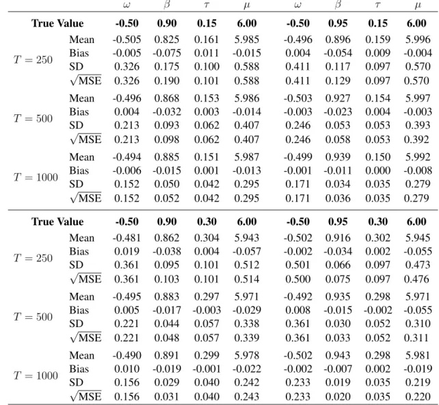
3.4 Monte Carlo experiment . . . 57
3.4.1 Finite sample behavior of the ML estimator . . . 57
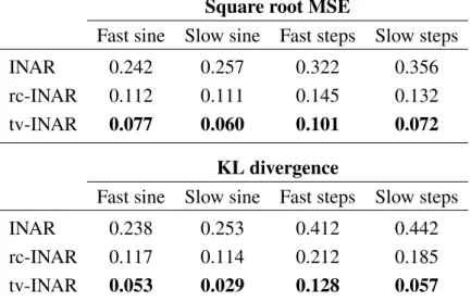
3.4.2 Filtering under misspecification . . . 59
3.5 Application to crime data . . . 61
3.5.1 In-sample results . . . 61
3.5.2 Forecasting results . . . 64
3.6 Conclusion . . . 65
Appendices 67 3.A Derivatives of the predictive log-likelihood . . . 67
3.B Proofs . . . 67
3.C Technical lemmas . . . 72
4 Accelerating GARCH and Score-Driven Models 75 4.1 Introduction . . . 75
4.2 Accelerating GARCH model . . . 76
4.3 Accelerating Score-Driven models . . . 79
4.4 Optimality properties . . . 81
4.4.1 A general updating mechanism . . . 81
4.4.2 Optimality of score innovations . . . 82
4.4.3 Relative optimality . . . 85
4.5 Monte Carlo experiment . . . 86
4.6 Empirical application to US stock returns . . . 89
4.7 Application to US inflation . . . 93
4.7.1 A fat tailed aGAS location model . . . 93
4.7.2 Empirical application . . . 95
4.7.3 Pseudo out-of-sample forecasts . . . 98
Appendices 101 4.A Proofs . . . 101
5 Conclusion 105
2.2.1 Filtered paths of the Beta-t-GARCH variance for different initializations. 12 2.2.2 Parameter region that satisfies sufficient invertibility conditions for the
Beta-t-GARCH model. . . 14
2.6.1 Estimated parameter region for the Beta-t-GARCH model using the S&P 500 stock index. . . 28
2.6.2 Estimated parameter region for the Beta-t-GARCH model with 95% con-fidence bounds. . . 29
2.6.3 Estimated parameter region for the US unemployment claims time series. 32 2.6.4 Estimated parameter region for the US consumer price inflation. . . 34
3.2.1 Impact of past observations and past survival probabilities on the score innovation . . . 50
3.4.1 Confidence bounds for the filtered survival probability obtained from the simulated series . . . 60
3.5.1 Monthly number of offensive conduct reports in Blacktown with empiri-cal autocorrelation functions . . . 62
3.5.2 Filtered survival probability with confidence bounds from the Blacktown crime time series . . . 63
4.2.1 Filtered variance from a simulated series for different values ofαt . . . . 78
4.2.2 Path of the filteredαt . . . 78
4.5.1 Realization of size1000from the DGP . . . 87
4.5.2 Filtered parameters obtained from the simulation experiment . . . 89
4.6.1 Percentage of series where each model outperforms the others for differ-ent kurtosis levels . . . 91
4.6.2 Boxplots of the Kurtosis distribution . . . 91
4.7.1 Impact of standardized observations on the score innovations . . . 95
4.7.3 Filtered aGAS parameters obtained from the US inflation series . . . 97 4.7.4 Filtered means for different time periods obtained from the US inflation
2.6.1 Beta-t-GARCH estimates and invertibility conditions for several stock in-dexes. . . 30 3.4.1 Summary statistics of the sample ML estimator distribution obtained from
the simulation experiment . . . 58 3.4.2 MSE and KL divergence between the true DGP and the models . . . 60 3.5.1 Specification of the models . . . 62 3.5.2 ML estimate of the models obtained from the Blacktown crime time series 63 3.5.3 Forecast MSE and log score criterion from the crime time series . . . 64 4.5.1 MSE between the filtered means and the true mean . . . 88 4.6.1 Number and the percentage of series in the S&P 500 index where each
Gaussian model outperforms the others. . . 90 4.6.2 Number and the percentage of series in the S&P 500 index where each
Student-t model outperforms the others. . . 93 4.7.1 Description of the models estimated for the US inflation series . . . 96 4.7.2 Estimated of the models obtained from the US inflation series . . . 96 4.7.3 FMSE and FMAE obtained from the last 100 observations of the US
Introduction
1.1
Overview
Time series data are encountered in most fields of empirical science as phenomena are typically observed sequentially over time. Examples range from the number of sunspots, or the water flow of a river in natural sciences to the number of inhabitants of a city, or the returns of a financial index in social sciences. The main assumption behind time series analysis is that past observations contain information about future observations. The idea is therefore to exploit this information and obtain more accurate predictions of future outcomes. Statistical modeling plays a key role in time series analysis as it summarizes the relevant information in the data and provides a probabilistic representation of the phenomenon of interest.
Statistical modeling of time series data has a long history. The first applications of autoregressive models go back to Yule (1927). Box and Jenkins (1970) provided a uni-fied approach to specification, estimation, diagnostic checking and forecasting of Inte-grated Autoregressive Moving Average (ARIMA) models. ARIMA models represent a milestone for time series modeling and their main justification rests on the Wold decom-position theorem (Wold, 1938). Several extensions of the ARIMA framework have been proposed over the years. Examples include the vector autoregressive model, Sims (1980), and the cointegration analysis of Engle and Granger (1987). A limitation of the ARIMA approach and its extensions is that they describe the linear dependence in the data but they do not explicitly take into account possible nonlinearities. This may be too restrictive in some situations of practical interest. For this reason, in the late 70s researchers started focusing on nonlinear time series models. One of the firsts to consider a nonlinear model was Tong (1978), introducing the class of Threshold Autoregressive (TAR) models. TAR
models allow the conditional mean of the process to depend on past observations in a nonlinear fashion. Nonlinear models come in different forms and shapes as nonlinearities can be introduced in different ways. A typical approach that produces nonlinear specifica-tions is to allow time variation in some features of the probability distribution of interest, i.e. some parameters. A well know example is to have time dependence in the variance of the observations. Popular models with dynamic variance are the Generalized Autoregres-sive Conditional Heteroscedastic (GARCH) model of Engle (1982) and Bollerslev (1986) and the Stochastic Volatility (SV) model of Taylor (1986). These models have been suc-cessfully employed in Econometrics and Finance to describe the well known volatility clustering often observed in financial asset returns.
Most time-varying parameter models can be classified in two categories: observation-driven and parameter-observation-driven models (Cox, 1981). In observation-observation-driven models, the pa-rameter of interest is made time-varying considering a stochastic processes where the source of randomness comes from past observations. Whereas, in parameter-driven mod-els, the time-varying parameter is specified as a stochastic process with its own source of error. In the context of volatility models, the GARCH model is an example of observation-driven model as the source of randomness is provided by past squared observations. On the other hand, the SV model is an example of parameter-driven model as the dynamic variance is driven by a latent autoregressive process. In most situations, as also in the case of the GARCH and the SV model, these two classes of models play equivalent roles. Their goal is to enable some features of the distribution of the variable of interest to change over time and, in this way, capture some form of dependence in the data. However, their statis-tical properties are quite different. Observation-driven models have the great advantage that they can be easily estimated since the likelihood function is available in closed form through a prediction error decomposition. Therefore, only standard optimization methods are needed to perform likelihood-based inference. Instead, in parameter-driven models, the likelihood function is usually not in closed form as it contains integrals with no ana-lytical solutions. Therefore, estimation is much more challenging from a computational point of view and time-consuming simulation-based methods are usually required. Some rare exceptions with close form solutions exist, see for example the Markov Switching models where the Hamilton filter can be employed (Hamilton, 1989).
In parameter-driven models, the time-varying parameter is typically specified as an au-toregressive process where the innovation is an independently and identically distributed (i.i.d.) sequence of Gaussian random variables. On the other hand, the specification of observation-driven models is often based on intuition. For instance, to make the variance time-varying it makes sense to consider a linear combination of squared past observations;
this leads to the well known GARCH model. However, sometimes it is not clear which function of the past observations to use and an intuitive choice may not always be the best option. Creal et al. (2013) and Harvey (2013) proposed an updating equation where the innovation is given by the score of the conditional distribution of the observations. This approach provides a general framework to specify the time-varying parameter in an observation-driven setting. The resulting class of models is known as Generalized Au-toregressive Score (GAS) models. Besides being intuitive, the use of the score as driving mechanism to update time-varying parameters is also justified by an optimality reasoning (Blasques et al., 2015). Since its introduction, the GAS framework has been successfully employed to develop dynamic models in econometrics and time series analysis, see for instance Salvatierra and Patton (2015), Harvey and Luati (2014) and Creal et al. (2011). It also turns out that many existing observation-driven models are in fact GAS models. Examples include the GARCH model and, in the context of integer-valued time series, the Poisson autoregressive model of Davis et al. (2003). For a more detailed discussion see Creal et al. (2013).
In this thesis, we address different aspects of observation-driven time series modeling including model specification and statistical inference. These two aspects are particularly relevant from a practical perspective as an appropriate specification of the model and a reliable inferential procedure are two of the main ingredients to obtain an accurate prob-abilistic representation of the time series of interest. The focus of the thesis is mostly on score-driven models though general results for observation-driven models are considered in Chapter 2. In particular, the second chapter of the thesis is concerned with model esti-mation of observation-driven models, whereas the third and fourth chapters are concerned with model specification in the setting of score-driven models. The 3 main chapters of the thesis are self contained and they can be read separately. In the following, we provide a brief outline for each chapter of the thesis. More detailed outlines can be found at the beginning of each chapter.
The first line of research, Chapter 2, concerns the consistency of likelihood-based inference for observation-driven models. One of the key steps to ensure the reliabil-ity of the Maximum Likelihood (ML) estimator is the study of the asymptotic behavior of the filtered time-varying parameter, i.e. the time-varying parameter recovered using the observed data. In the context of Quasi Maximum Likelihood (QML) estimation of GARCH-type models, Straumann and Mikosch (2006) proposed to rely on Theorem 3.1 of Bougerol (1993) to ensure the asymptotic stability of the filtered parameter, which is known as invertibility. Compared to previous research, their approach allows us to handle nonlinearities in the recursion of the filtered parameter. However, the required
invert-ibility conditions often impose restrictions on the parameter space that are unfeasible to be checked in practice. This occurs because these invertibility conditions depend on the properties of the Data Generating Process (DGP) that are unknown. Wintenberger (2013) noted this problem for the EGARCH model of Nelson (1991) and proposed to replace the unfeasible conditions with a feasible empirical invertibility condition. This method deliv-ers a consistent QML estimator for the EGARCH model. We note that this problem is not a peculiarity of the EGARCH model but a general problem for observation-driven models with nonlinearities in the filtered parameter recursion. Therefore, often, the asymptotic theory can be ensured only for either degenerate or very small parameter regions that are unrealistic in empirical applications. As examples, we consider the Beta-t-GARCH model of Harvey (2013) and Creal et al. (2013), the location model of Harvey and Luati (2014) and the autoregressive model of Blasques et al. (2014b) and Delle Monache and Petrella (2016). We build on the work of Wintenberger (2013) and deliver a general the-ory for observation-driven models that ensures the consistency of the ML estimator under feasible invertibility conditions. The resulting theory is shown to cover applications of practical interest such as modeling of financial stock returns and macroeconomic vari-ables. An appealing feature of our theoretical results is that they hold also in the case of model misspecification. In this situation, the consistency is proved with respect to a pseudo-true parameter.
The second line of research, Chapter 3, concerns integer-valued time series modeling. Over the last few years, there has been an increasing interest in modeling time series with non-continuous response variables. This due to the fact that many observed variables take values in a discrete support and models for continuous variables are not suited in these sit-uations. One of the most popular class of models for count time series data is the class of Integer-valued Autoregressive (INAR) models introduced by Al-Osh and Alzaid (1987) and McKenzie (1988). INAR models can be seen as a discrete version of the continu-ous response AR models as they share several common properties. An appealing feature of INAR models is their interpretation as birth-death processes: at each time period the count is given by the sum between the number of new born elements and the number of elements surviving from the previous period. Assuming a constant survival probability can be too restrictive in many situations as real time series often exhibit changes in their behavior over time. Therefore, allowing different persistence levels in different time pe-riods can be useful to better describe the observed variable and enhance the forecasting performance of the model. We propose a novel dynamic specification for the surviving probability. The peculiarity of our approach is to consider an observation-driven dynamic for the surviving probability based on the GAS framework. The resulting class of
mod-els is appealing from several prospectives. First, the proposed dynamic coefficient is very effective in capturing smooth changes in the survival probability. We illustrate this through a simulation study designed in a misspecified setting where the survival proba-bility follows different deterministic paths. Second, the estimation of the model can be easily performed by maximum likelihood using standard optimization algorithms as for the classic INAR model. Finally, the proposed class of models allows us to consider gen-eral distributions for the new born process without additional difficulties in the derivation of the model specification and estimation. One of the main contributions of this chapter is the study of some statistical properties of the proposed model. In particular, we show the consistency of ML estimation for the static parameters and for the predictive probability mass function. Furthermore, we also provide an empirical application to a crime time series to illustrate how our class of models can be useful in practice.
The third and last line of research, Chapter 4, concerns model specification in the framework of GAS models. As mentioned before, in the GAS framework, the time-varying parameter is specified as an autoregressive process where the innovation is given by the score of the predictive likelihood. As discussed in Blasques et al. (2015), the GAS updating mechanism can be seen as a sort of Newton Raphson algorithm where the score provides the direction of the updating step. We propose to allow the magnitude of the updating step to be time-varying. The idea behind having time variation in the size of the step is related to the amount of local information in the data. In some time periods, the most recent observations can be very informative to predict future observations, whereas, in other periods, this may not be the case. Therefore, in such situations, we would like the time-varying parameter to be updated quickly when the data is informative and slowly when the data is not informative. The specification we introduce to capture time variation in the magnitude of the GAS updating step is given by a weighted autocorrelation of past GAS innovations. This has an intuitive interpretation: the amount of local information in the data is determined by the dependence of past score innovations. We perform a simu-lation study as an illustrative example of this idea and show the benefits that our approach can provide. Furthermore, in the spirit of Blasques et al. (2015), we derive an optimality justification for the proposed method in terms of Kullback-Leibler (KL) divergence reduc-tion between the true and unknown condireduc-tional distribureduc-tion and the postulated statistical model. Finally, some empirical examples considering volatility and location models are presented. In particular, in the context of volatility models, we derive an extension of the GARCH model and perform an empirical study using the stock returns of the S&P 500 financial index. Whereas, in the context of location models, we specify a fat tailed model and illustrate an empirical application to the US consumer price inflation series. Overall,
the empirical results show promising results both in-sample and out-of-sample.
1.2
Main contributions of the thesis
In the following, we summarize the main original contributions of the thesis.
Chapter 2.
1. Feasible consistency conditions for ML estimation of a wide class of observation-driven time series models are derived.
2. The consistency of the ML estimator for the Beta-t-GARCH model is proved under a testable invertibility condition.
3. The theory developed in the chapter is shown to be useful also outside the frame-work of GARCH-type models. This is done by means of two examples in the context of location models.
Chapter 3.
1. A new class of observation-driven INAR models with dynamic survival probabil-ity is introduced. Estimation and forecasting procedures of the proposed class of models is presented.
2. The consistency of ML estimation of the static parameter vector and the conditional probability mass function is proved.
3. The flexibility of the proposed class of models is illustrated through a simulation study. Furthermore, an empirical application to a crime time series is provided.
Chapter 4.
1. An extension of the GAS framework is proposed. This extension introduces time variation in the updating equation of score-driven models.
2. An optimality argument that justifies the proposed specification of the time-varying parameter update is derived.
3. Empirical illustrations in economics and finance to show how the proposed ap-proach can be useful in practice are presented. More specifically, applications to financial stock returns and the US inflation series are considered.
Feasible Invertibility Conditions for
Maximum Likelihood Estimation of
Observation-Driven Models
2.1
Introduction
Observation-driven models are widely employed in time series analysis and economet-rics. These models feature time-varying parameters that are specified through a Stochas-tic Recurrence Equation (SRE) driven by past observed elements of the time series. A well know example of observation-driven models is the class of GARCH-type models. Observation-driven models are widely used also outside the context of volatility models; see for instance the Dynamic Conditional Correlation (DCC) model of Engle (2002), the time-varying quantile model of Engle and Manganelli (2004), the dynamic copula mod-els of Patton (2006), the score modmod-els of Creal et al. (2013) and the time-varying location model of Harvey and Luati (2014).
The asymptotic theory of the QML estimator for GARCH-type models has attracted much attention. Lumsdaine (1996) and Lee and Hansen (1994) obtained the consistency and asymptotic normality of the QML estimator for the GARCH(1,1). Berkes et al. (2003) generalized their results to the GARCH(p,q). Among others, Francq and Zakoian (2004) and Robinson and Zaffaroni (2006) weakened the conditions for consistency and asymptotic normality and extended the results to a larger class of models. Straumann and Mikosch (2006) provided a very general approach to handle nonlinearities in the variance recursion. Their theory relies on the work of Bougerol (1993) to ensure the invertibil-ity of the filtered time-varying variance and delivers asymptotic results that are subject to
some restrictions on the parameter region where the QML estimator is defined. The sever-ity of these restrictions typically depends on the degree of nonlinearsever-ity in the recurrence equation.
We note that, in practical applications, the invertibility conditions of Straumann and Mikosch (2006) often fail to be guaranteed. We will illustrate this issue through some empirical examples featuring the Beta-t-GARCH model of Harvey (2013) and Creal et al. (2013), the autoregressive model with dynamic coefficient of Blasques et al. (2014b) and Delle Monache and Petrella (2016) and the fat-tailed location model of Harvey and Luati (2014). The main problem lies on the fact that these conditions are empirically unfeasible as they depend on the unknown DGP. This leads researchers to rely on feasible conditions that are typically only satisfied in either degenerate or very small parameter regions that are too restrictive for practical situations. To handle this issue and ensure the asymptotic theory of the QML estimator of the EGARCH(1,1) model of Nelson (1991), Wintenberger (2013) proposed to stabilize the inferential procedure by restricting the optimization of the quasi-likelihood function to a parameter region that satisfies an empirical version of the required invertibility conditions considered in Straumann and Mikosch (2006). This method provides a consistent QML estimator for the EGARCH(1,1) model.
In the literature, there are also consistency proofs for observation-driven models with nonlinear filters that do not rely on the invertibility concept of Straumann and Mikosch (2006), see for instance Harvey (2013), Harvey and Luati (2014) and Ito (2016). However, these results appeal to Lemma 2.1 of Jensen and Rahbek (2004) and rely on the very restrictive and non-standard assumption that the true value of the unobserved time-varying parameter is known at timet= 0. Unlike Jensen and Rahbek (2004), who carefully show that they do not need to impose this assumption in their non-stationary GARCH paper, this crucial issue is typically not addressed. As discussed in Wintenberger (2013) and Sorokin (2011), invertibility is not just a technical assumption as the lack of knowledge of the true initial value of the time-varying parameter att = 0can lead to the impossibility of recovering asymptotically the true time-varying parameter even knowing the true vector of static parameters. Furthermore, besides the invertibility issue, the results based on Lemma 2.1 of Jensen and Rahbek (2004) are only valid under the correct specification of the model and assuming that the likelihood function is maximized on an arbitrary small neighborhood around the true parameter value.
In this chapter, we extend the stabilization method of Wintenberger (2013) to a large class of observation-driven models and prove the consistency of the resulting ML estima-tor. The resulting theory provides feasible invertibility conditions that allow us to drop the unrealistic assumption that the time-varying parameter is known att= 0. Our consistency
results hold for both correctly specified and misspecified models. In the latter case consis-tency is considered with respect to a pseudo-true parameter that has the interpretation of minimizing a marginal KL divergence between the true unknown conditional distribution and the conditional distribution of the postulated model. Additionally, we derive a test and confidence bounds for the “true” unfeasible parameter region. Our results cover a very wide class of models including ML estimation of GARCH-type models. In financial applications, maximum likelihood estimation for GARCH-type models is often preferred to QML estimation as the time series exhibit fat-tails and asymmetry. In this context, we provide an example of how our results can be useful in practice. In particular, we prove the consistency of the ML estimator for the Beta-t-GARCH model of Harvey (2013) and Creal et al. (2013). The usefulness of our theoretical results is further illustrated consid-ering two example in the context of dynamic location model. In particular, we discuss the implications of our results considering the dynamic autoregressive model of Blasques et al. (2014b) and Delle Monache and Petrella (2016) and the fat-tailed location model of Harvey and Luati (2014).
The chapter is structured as follows. Section 2.2 motivates the theory presented in the chapter with an empirical application for which the invertibility conditions used in Straumann and Mikosch (2006) are too restrictive. Section 2.3 introduces the notion of invertibility of the filter and analyzes it in the context of the class of observation-driven models studied in this chapter. Section 2.4 presents the asymptotic results. Section 2.5 derives an invertibility test for the filter and obtains confidence bounds for the parameter space of interest. Section 2.6 shows the practical importance of the asymptotic results through some empirical illustrations. Section 2.7 concludes.
2.2
Motivation
Consider the Beta-t-GARCH model introduced by Harvey (2013) and Creal et al. (2013) for a sequence of financial returns {yt}t∈Z with time-varying conditional volatility and leverage effects, yt = p ftεt and ft+1 =ω+βft+ (α+γdt) (v+ 1)y2 t (v−2) +y2 t/ft , (2.1)
where {εt}t∈Z is an i.i.d. sequence of standard Student-t random variables with v > 2 degrees of freedom and dt is a dummy variable that takes value dt = 1 if yt ≤ 0and dt = 0 otherwise. In order to perform ML estimation of the model, the observed data
{yt}Tt=1are used to obtain the filtered time-varying parameterfˆt(θ)as ˆ ft+1(θ) =ω+βfˆt(θ) + (α+γdt) (v+ 1)y2 t (v−2) +y2 t/fˆt(θ) , t∈N,
where the recursion is initialized atfˆ0(θ)∈ [0,+∞). The invertibility concept of Strau-mann and Mikosch (2006) is concerned with the stability of fˆt(θ). In particular, it en-sures that asymptotically the filtered parameterfˆt(θ)does not depend on the initialization
ˆ
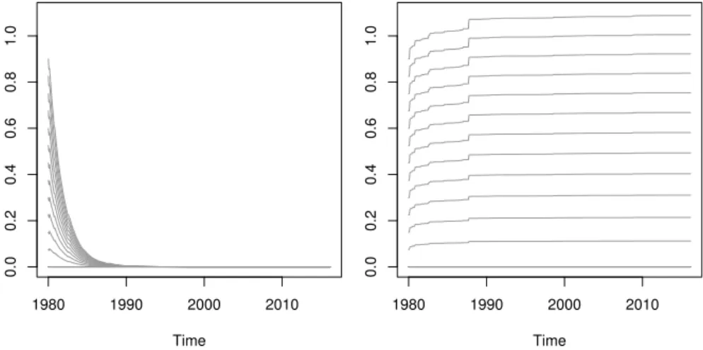
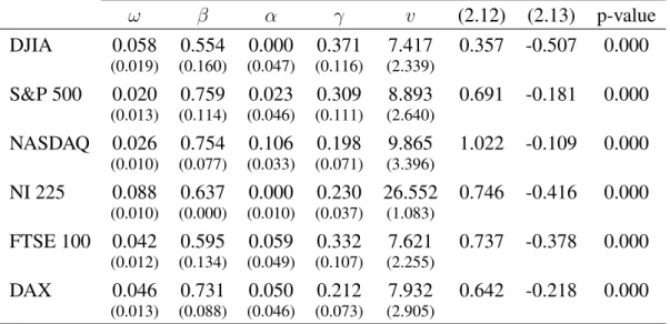
f0(θ). Figure 2.2.1 illustrates the importance of the invertibility of the filter. The plots show differences between filtered volatility paths obtained from the S&P 500 returns for different initializationsfˆ0(θ). The left panel shows a situation where the filter is invert-ible and hence the effect of the initializationfˆ0(θ)onfˆt(θ)vanishes as t increases. The right panel shows that the effect of the initialization does not vanish when the filter is not invertible. Time 1980 1990 2000 2010 0.0 0.2 0.4 0.6 0.8 1.0 Time 1980 1990 2000 2010 0.0 0.2 0.4 0.6 0.8 1.0
Figure 2.2.1: Filtered variance paths for different initializations and using the S&P 500 time series. Differences are with respect to the filter initialized atfˆ0(θ) = 0.1. In the first plot, the vector of static parameters is selected to satisfy the invertibility conditions. In the second plot, a vector of static parameters that does not satisfy the invertibility conditions is considered.
From a ML estimation perspective, the lack of invertibility of the filter also poses fundamental problems. Without invertibility, even asymptotically, the likelihood function depends on the initialization and hence this may lead the ML estimator to converge to different points when different initializations are considered. Furthermore, we may also be in a situation where we have a consistent estimator for the static parameter vectorθbut we may not be able to consistently estimate the time-varying parameter. This considera-tion comes naturally from the fact that lack of invertibility can lead to the impossibility
of recovering the true path of the time-varying parameter even when the true vector of static parameters θ0 is known, see Wintenberger (2013) and Sorokin (2011) for a more
detailed discussion. As we shall see, the following condition on the parameter regionΘ
is sufficient for invertibility, and hence ensures the reliability of the ML estimator, Elog β+ (α+γdt) (v+ 1)y4 t ((v−2)¯ω+y2 t) 2 <0, ∀θ∈Θ, (2.2) whereω¯ =ω/(1−β). However, in practice, it is not possible to evaluate the expectation in (2.2) as it depends on the unknown DGP. Note that this is true even when the model is correctly specified as the true parameter vectorθ0 is unknown. Therefore, the derivation
of the regionΘhas to rely on feasible sufficient conditions to ensure (2.2). As we shall see in Section 2.6, assuming either correct specification or thatythas a symmetric probability distribution around zero1, we can obtain the following sufficient invertibility condition that does not depend onyt
1
2log|β+ (α+γ)(v+ 1)|+ 1
2log|β+α(v+ 1)|<0.
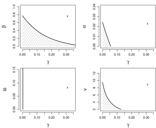
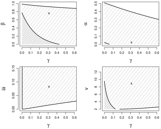
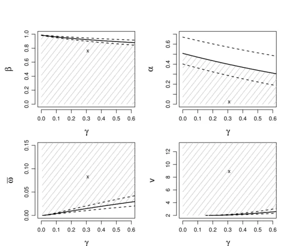
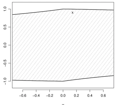
Unfortunately, Figure 2.2.2 suggests that the setΘobtained from such a sufficient con-dition is too small for empirical applications. In particular, Figure 2.2.2 highlights that a typical ML point estimate lies far outsideΘ. This specific point estimate is obtained from monthly log-differences of the S&P 500 financial index from January 1980 to April 2016. Figure 2.2.2 might indicate that the filter is not stable or invertible. However, as we shall see in Section 2.6, this seems not to be the case. This point estimate lies well inside the estimated region for an invertible filter. The tests and confidence bounds developed in Section 2.5 further confirm this claim.
As we will discuss in Section 2.6, the problem illustrated in Figure 2.2.2 is not specific to this sample of data. Different samples of financial returns produce similar point esti-mates that lie also outsideΘ. This problem is also not specific for the class of conditional heteroscedastic models. We illustrate this point considering the autoregressive model of Blasques et al. (2014b) and Delle Monache and Petrella (2016) and the location model of Harvey and Luati (2014). We find that, in general, the typical invertibility conditions needed to ensure the consistency of the ML estimator, which are considered for instance in Straumann and Mikosch (2006), Straumann (2005) and Blasques et al. (2014a), lead often to a parameter region that is too small for practical purposes. In contrary, the estimation method of Wintenberger (2013), proposed for the QML estimator of the EGARCH(1,1)
0.00 0.10 0.20 0.30 0.0 0.2 0.4 0.6 0.8 1.0 γ β x 0.00 0.10 0.20 0.30 0.00 0.01 0.02 0.03 0.04 γ α x 0.00 0.10 0.20 0.30 0.00 0.05 0.10 0.15 γ ω x 0.00 0.10 0.20 0.30 2 4 6 8 10 12 γ v x
Figure 2.2.2: The shaded area identifies the parameter regionΘ that satisfies sufficient conditions for invertibility. Crosses locate the point estimate of the parameters of the Beta-t-GARCH model.
model, can provide a parameter region large enough for practical applications. In Sec-tion 2.3 and SecSec-tion 2.4, we will generalize the method of Wintenberger (2013) to ML estimation of a wide class of observation-driven models.
2.3
Invertibility of observation-driven filters
Let the observed sample of data {yt}Tt=1 be a subset of the realized path of a random
sequence{yt}t∈Z with elements taking values inY ⊆ R and having and unknown con-ditional density po(y
t|yt−1), where yt−1 denotes the entire past of the process yt−1 =
{yt−1, yt−2, ...}. Consider now the following parametric observation-driven time-varying
parameter model postulated by the researcher
yt|ft∼p(yt|ft, θ), (2.3) ft+1 =φ(ft, Ytk, θ), t∈Z, (2.4)
whereθ ∈ Θ ⊆ Rp is a vector of static parameters, ft is a time-varying parameter that takes values in Fθ ⊆ R, φ is a continuous function from Fθ × Yk × Θ into Fθ, Ytk is a vector containingk lags of the observed time series Yk
t = (yt, yt−1, ..., yt−k)T, and p(·|ft, θ)is a conditional density function such that(y, f, θ)7→p(y|f, θ)is continuous on
Y × Fθ×Θ.
As mentioned before, we also address the possibility of having a misspecified model. More specifically, we allow the parametric model in (2.3) and (2.4) to be fully misspec-ified. This means that both the dynamic specification offt and the conditional density p(·|ft, θ)can be misspecified. Note that a true time-varying parameter ft may not even exist as we only assume that a true conditional densitypo(·|yt−1)exists. When we assume
correct specification, the DGP{yt}t∈Z satisfies the model’s equations (2.3) and (2.4) for θ = θ0 and we denote with fto the true time-varying parameter. In this situation, we have thatpo(·|yt−1) = p(·|fo
t, θ0). Despite the possibility of model misspecification, it is worth noting that the model in (2.3) and (2.4) is very general and it covers a wide range of observation-driven models. Besides many GARCH-type models, this class of mod-els includes location modmod-els as in Harvey and Luati (2014), Multiplicative Error Memory (MEM) models as in Engle (2002), Autoregressive Conditional Duration models as in En-gle and Russell (1998), Autoregressive Conditional Intensity models as in Russell (2001) and Poisson autoregressive models as in Davis et al. (2003).
An important advantage of observation-driven models is that the likelihood function is analytically tractable and can be written in closed form as the product of conditional density functions. We consider the convention that the observations are available from timet = 1−k. Using the observed data, the filtered parameterfˆt(θ)that enters in the likelihood function is obtained through the following SRE
ˆ
ft+1(θ) =φ( ˆft(θ), Ytk, θ), t∈N, (2.5) where the recursion is initialized att = 0withfˆ0(θ) ∈ Fθ. Note that the setFθ, where the time-varying parameter takes values, is indexed byθ ∈ Θ. As we will see for the Beta-t-GARCH model, this can be relevant in practice when dealing with specific models to weaken invertibility conditions. The ML estimator is formally defined as
ˆ
θT = arg max θ∈Θ
ˆ
whereLˆT(θ)denotes the log-likelihood function evaluated atθ ∈Θ, ˆ LT(θ) = T−1 T X t=1 ˆ lt(θ), (2.7) andˆlt(θ) = logp(yt|fˆt(θ), θ).
One of the difficulties in ensuring the consistency of the ML estimator is related to the recursive nature of the time-varying parameter and the consequent need of initializing the recursion in (2.5). In particular, it is important to note that the sequence{fˆt(θ)}t∈N as well as the sequence {ˆlt(θ)}t∈N are both non-stationary. Therefore, the study of the limit behavior of {fˆt(θ)}t∈N is a natural requirement to ensure an appropriate form of convergence of the log-likelihood functionLˆT(θ). The required stability of{fˆt(θ)}t∈Nis known as invertibilty.
Bougerol (1993) provides well known conditions for the filtered sequence{fˆt(θ)}t∈N initialized at timet = 0to converge exponentially fast almost surely (e.a.s.)2 to a unique
stationary and ergodic sequence {f˜t(θ)}t∈Z ast → ∞. In essence, this means that the effect of the initialization vanishes asymptotically at an exponential rate.3 More formally,
for any givenθ ∈ Θand under appropriate conditions, Theorem 3.1 in Bougerol (1993) shows that
|fˆt(θ)−f˜t(θ)| e.a.s.
−−−→0, t−→ ∞,
for any initializationfˆ0(θ)∈ Fθ. Straumann and Mikosch (2006) make use of Bougerol’s theorem and note that the e.a.s. convergence stated above is sufficient for the invertibil-ity of the filter4. Their definition of invertibility is closely related to the definition of invertibility in Granger and Andersen (1978) as it implies thatfo
t isyt−1measurable. We mention that the stationary and ergodic limit sequence is denoted by f˜t(θ) and not ft(θ) to stress the fact that the stochastic properties of f˜t(θ) are different from the stochastic properties of the sequenceft(θ)that follows the model’s equations (2.3) and (2.4). This becausef˜t(θ)is driven by past random variables of the DGP, which does not follow the model’s equations. Under correct specification, we have thatf˜t(θ)has the same stochastic properties offt(θ)only whenθ = θ0 as the DGP follows the model equations
only atθ0. For more details see Straumann and Mikosch (2006) and Wintenberger (2013). 2
A sequence of non-negative random variables{xt}t∈Nis said to converge e.a.s. to zero if there exists a
constantγ >1such thatγt
xt
a.s.
−−→0 astdiverges.
3In the context of correctly specified models this implies that the true path{fo
t}t∈Zcan be asymptotically
recovered asfˆt(θ0)converges tof˜t(θ0) =ftoa.s. astdiverges.
4
Straumann and Mikosch (2006) say that the model is invertible iffˆt(θ0)converges in probability tof˜to
It is also worth stressing the fact that, even if the model is assumed to be well specified, different conditions are required to establish invertibility and stationarity. As shown by Sorokin (2011) for some GARCH-type models, we can have that for a givenθ0, the model
in (2.4) admits a stationary solution but lacks invertibility. In these situations, the true sequence {fˆt(θ0)}t∈N can exhibit chaotic behaviors and the true path of fto cannot be recovered asymptotically even when the true vector of static parametersθ0 is known. See
also the discussion in Wintenberger (2013). For this reason, ensuring the invertibility of the filtered parameter is not merely a technical requirement but an important ingredient to ensure the reliability of the inferential procedure.
The invertibility of the sequence {fˆt(θ)}t∈N evaluated at a single parameter value θ ∈ Θis not enough to ensure an appropriate convergence of the log-likelihood func-tion overΘ. This happens naturally because the likelihood function depends on the func-tional sequence {fˆt}t∈N. In this regard, Wintenberger (2013) introduced the notion of continuous invertibility for GARCH-type models to ensure the uniform convergence of the filtered volatility. In our case, accounting for the continuity of the function φ, the elements of the sequence{fˆt}t∈Ncan be considered as random elements in the space of continuous functionsC(Θ,FΘ)that map fromΘintoFΘ,FΘ :=S
θ∈ΘFθ, equipped with
the uniform normk · kΘ, wherekfkΘ = supθ∈Θ|f(θ)| for anyf ∈ C(Θ,FΘ). We say
that the filter{fˆt}t∈Nis invertible if for any initializationfˆ0 ∈C(Θ,FΘ)
kfˆt−f˜tkΘ−−−→e.a.s. 0, t−→ ∞,
where {f˜t}t∈Z is a stationary and ergodic sequence of random functions. Also in this case, note the relation with the invertibility concept in Granger and Andersen (1978) as the invertibility implies that the stochastic functionf˜tisyt−1 measurable.
Proposition 2.3.1 presents sufficient conditions for the invertibility of{fˆt}t∈N. As in Straumann (2005), Straumann and Mikosch (2006) and Wintenberger (2013), the con-ditions we consider are based on Theorem 3.1 of Bougerol (1993). First, we define the stochastic Lipschitz coefficientΛt(θ)as
Λt(θ) := sup f∈Fθ φ˙(f, Y k t , θ) , whereφ˙(f, Yk t , θ) =∂φ(f, Ytk, θ)/∂f.
Proposition 2.3.1. Assume{yt}t∈Zis a stationary and ergodic sequence of random vari-ables. Moreover, let the following conditions hold
(ii) Esupθ∈Θsupf∈FΘlog+
φ˙(f, Ytk, θ) <∞.
(iii) log Λ0(θ)is a.s. continuous onΘandElog Λ0(θ)<0for anyθ ∈Θ.
Then, the functional sequence {fˆt}t∈N defined in (2.5) converges exponentially almost surely and uniformly to a unique stationary and ergodic sequence{f˜t}t∈Z, i.e.
kfˆt−f˜tkΘ
e.a.s.
−−→0 as t→ ∞, for any initializationfˆ0 ∈C(Θ,FΘ).
Proposition 2.3.1 not only ensures the convergence of {fˆt}t∈N to a stationary and ergodic sequence{f˜t}t∈Z but also that this sequence is unique and therefore the initial-izationfˆ0 is irrelevant asymptotically. Note also that Proposition 2.3.1 holds irrespective
of the correct specification of the model as it only requires that the data are generated by a stationary and ergodic process. Often, in practical situations, the so-called ‘contrac-tion condi‘contrac-tion’ stated in (iii) is the most restrictive condi‘contrac-tion and it also imposes the most severe constraints on the parameter spaceΘ.
Remark 2.3.1. When the model is correctly specified and conditions (i)-(iii) of Propo-sition 2.3.1 hold, then the filter evaluated at θ0 ∈ Θ converges to the true unobserved
time-varying parameter{fo
t}t∈Z, i.e. |fˆt(θ0)−fto|
e.a.s.
−−→0 as t→ ∞, for any initializationfˆ0(θ0)∈ Fθ0.
Remark 2.3.1 highlights an important implication of Proposition 2.3.1 under correct specification. We obtain that, knowing the vector of static parametersθ0, the true path of
fo
t can be recovered asymptotically.
2.4
Maximum likelihood estimation
The invertibility of the filter obtained from Proposition 2.3.1 can be used to establish the consistency of the ML estimator defined in (2.6) over the parameter space Θ. We also discuss how the invertibility allows us to ensure the consistency of the plug-in estimators
ˆ
ft(ˆθT) and p(y|fˆt(ˆθT),θˆT), y ∈ Y, for the time-varying parameter and the conditional density function. After the derivation of these results, we obtain the consistency of the ML estimator replacing the unfeasible parameter regionΘwith an estimated setΘˆT that
ensures an empirical version of the contraction conditionElog Λ0(θ) < 0. Finally, we study the case of model misspecification for the ML estimator based on the feasible pa-rameter regionΘˆT.
The subsequent results are subject to the stationarity and ergodicity of the data gen-erating process. In the case of correct specification, stationarity and ergodicity can be checked studying the properties of the DGP, see Blasques et al. (2014c) for sufficient conditions for a wide class of observation-driven processes. In the case of misspecifica-tion, instead of imposing that the data are generated by a specific stationary and ergodic process, we allow the data generating process to be any stationary ad ergodic process.
2.4.1
Consistency of ML estimation
The first consistency result we obtain is under the assumption of correct specification. We denote the log-likelihood function evaluated at the stationary limit of the filtered param-eterf˜tasLT(θ) = T−1PTt=1lt(θ), wherelt(θ) = logp(yt|f˜t(θ), θ), and we denote byL the functionL(θ) =El0(θ). The following conditions are considered.
C1: The data generating process, which satisfies the equations (2.3) and (2.4) with θ =
θ0 ∈Θ, admits a stationary and ergodic solution andE|l0(θ0)|<∞.
C2: For anyθ ∈Θ,l0(θ0) = l0(θ)a.s. if and only ifθ=θ0.
C3: Conditions (i)-(iii) of Proposition 2.3.1 are satisfied for the compact setΘ⊂Rp. C4: There exists a stationary sequence of random variables{ηt}t∈ZwithElog+|η0|<∞
such that almost surelykˆlt−ltkΘ≤ηtkfˆt−f˜tkΘfor anyt≥N,N ∈N.
C5: Ekl0 ∨0kΘ <∞.
ConditionC1ensures that the data are generated by a stationary and ergodic process and imposes an integrability condition on predictive log-likelihood, which is needed to apply an ergodic theorem. Condition C2 is a standard identifiability condition. Conditions C3 and C4 ensure the a.s. uniform convergence of LˆT to LT. Finally, Condition C5 ensures that Ln converges to an upper semicontinuous function L. As also considered in Straumann and Mikosch (2006), this final argument replaces the well known uniform convergence argument, namely, the uniform convergence ofLT toL. Note that Condition C5is weaker than the conditions typically needed for uniform convergence and in many cases it holds automatically asl0(θ)is bounded from above with probability 1. Theorem
Theorem 2.4.1. Let the conditionsC1-C5hold, then the ML estimator defined in (2.6) is
strongly consistent, i.e.
ˆ
θT
a.s.
−→ θ0, T −→ ∞
for any initializationfˆ0 ∈C(Θ,FΘ).
The proof is in the appendix. In Section 2.6, the strong consistency of the Beta-t-GARCH model is proved by checking these conditions.
Often, the main objective of time series modeling is to describe the dynamic behaviour of the observed data and predict future observations. For this reason, it is interesting to study the consistency of the estimation of the time-varying parameter fo
t and the con-ditional density function p(y|fo
t, θ0), y ∈ Y. This further highlights the importance of the invertibility of the filter as without invertibility it may be possible to estimate consis-tently the static parameters, as shown by Jensen and Rahbek (2004) for the non-stationary GARCH(1,1), but it may not be possible to estimate consistently the time-varying pa-rameter and the conditional density function. We consider plug-in estimates for the time-varying parameter, given byfˆt(ˆθT), and for the conditional density function, given by p(y|fˆt(ˆθT),θˆT),y∈ Y. The next result shows the consistency of these plug-in estimators. The consistency is obtained when bothtandT go to infinity. This is needed because asT grows we obtain the consistency of the static parameter estimator and ast grows, thanks to the invertibility of the filter, we obtain that the effect of the initializationfˆ0 becomes
negligible. To obtain the desired result, besides the consistency conditions employed in Theorem 2.4.1, we additionally impose some Lipschitz conditions.
L1: There is a stationary sequence of random variables{vt}t∈Zsuch that almost surely |f˜t(θ1)−f˜t(θ2)| ≤vtkθ1−θ2k, ∀ θ1, θ2 ∈Θ, t∈Z.
L2: For anyy ∈ Y there is a constantcy >0such that cy
p(y|f1, θ1)−p(y|f2, θ2)
≤ kθ1−θ2k+|f1−f2|, ∀ θ1, θ2 ∈Θandf1, f2 ∈ FΘ.
The vector normk · kcan be any vector norm. Corollary 2.4.1 below follows immediately from the Lipschitz condition on the filterL1and the Lipschitz condition on the conditional density functionL2.
Corollary 2.4.1. Let the conditionsC1-C5andL1hold, then the plug-in estimatorfˆt(ˆθT)
is consistent, i.e.
|fˆt(ˆθT)−fto| pr
Assume furthermore that alsoL2holds, then the plug-in estimatorp(y|fˆt(ˆθT),θˆT)is con-sistent, i.e. p(y|fˆt(ˆθT),θˆT)−p(y|fto, θ0) pr −→0, T → ∞, t→ ∞,
for anyy ∈ Yand any initializationfˆ0 ∈C(Θ,FΘ).
Corollary 2.4.1 shows that the time-varying parameterfo
t and the conditional density functionp(y|fo
t, θ0),y∈ Y, can be consistently estimated.
2.4.2
ML on an estimated parameter region
As discussed before, the Lyapunov conditionElog Λ0(θ) <0imposes some restrictions
on the parameter regionΘ. Furthermore, in situations whereΛ0(θ)depends onYk
0, these
restrictions cannot be checked as the expectation depends on the unknown DGP. Note that this is true even in the case of correct specification as the true parameterθ0 is unknown.
A possible solution is to obtain testable sufficient conditions such that Elog Λ0(θ) <
0 and define the set Θ accordingly. However, as discussed before, this often leads to very severe restrictions, reducing the setΘto a small region that is usually too small for practical applications. Therefore, a better alternative consists in checking the condition Elog Λ0(θ) < 0 empirically and define the ML estimator as the maximizer of the log-likelihood on an estimated parameter region. In the context of QML estimation, this approach have been proposed by Wintenberger (2013) to stabilize the QML estimator of the EGARCH(1,1) model of Nelson (1991). In this section we formally define this ML estimator and we prove its consistency for the general class of observation-driven models defined in (2.3). In Section 2.6, we show how these results can be relevant in practical applications.
We define a compact setΘˆT that satisfies an empirical version of the Lyapunov con-ditionElog Λ0(θ)<0as ˆ ΘT = ( θ∈Θ :¯ 1 T T X t=1 log Λt(θ)≤ −δ ) , (2.8)
whereΘ¯ ⊂Rp is a compact set andδ >0is an arbitrary small constant. We assume that the compact setΘ¯ is chosen in such a way that (f, y, θ) 7→ φ(f, y, θ)is a continuous on
FΘ¯ × Yk ×Θ¯ and(y, f, θ) 7→ p(y|f, θ)is continuous onY × FΘ¯ ×Θ¯. For notational
estimator on this empirical regionΘˆT is formally defined as ˆˆ θT = arg max θ∈ΘTˆ ˆ LT(θ). (2.9)
To ensure the consistency of this ML estimator in the case of correct specification the following conditions are considered.
A1: The DGP, which is given by the model in (2.3) and (2.4) with θ0 ∈ Θδ, admits a stationary and ergodic solution andE|l0(θ0)|<∞.
A2: Condition(i)and(ii)of Proposition 2.3.1 are satisfied for any compact subsetΘ⊆ Θ0. Moreover, the map θ 7→ log Λ0(θ) is almost surely continuous on Θ¯ and Eklog Λ0kΘ¯ <∞.
A3: ConditionsC2,C4andC5are satisfied for any compact subsetΘ⊆Θ0.
Note thatA1ensures stationarity, ergodicity and invertibility of the data generating pro-cess. This condition can be seen as the equivalent of the conditionC1in Theorem 2.4.1. The conditionA2imposes some assumptions onlog Λ0(θ). These assumptions are needed
to guarantee a certain form of convergence for the set ΘˆT and consequently ensure the continuous invertibilitykfˆt −f˜tkΘTˆ
e.a.s.
−−→ 0 as t → 0 for large enough T. Therefore, A2can be seen as the equivalent of C3in Theorem 4.1. Finally, A3, together with A2, is sufficient to ensure that asymptotically the identifiability conditionC2, the regularity conditionC4and the integrability conditionC5holds. The next theorem states the strong consistency of the ML estimator in (2.9) under correct specification.
Theorem 2.4.2. Let conditions A1-A3 hold, then the ML estimator defined in (2.9) is
strongly consistent, i.e.
ˆˆ
θT
a.s.
−→ θ0, T −→ ∞
for any initializationfˆ0 ∈C( ¯Θ,FΘ¯).
Theorem 2.4.2 generalizes Theorem 5 of Wintenberger (2013), which is specific to QML estimation of the EGARCH(1,1) model, to ML estimation of the wide class of observation-driven models specified in (2.3) and (2.4). The conditions required to ensure the strong consistency in Theorem 2.4.2 are feasible to be checked. This differs from other results in the literature such as Straumann and Mikosch (2006), Harvey (2013), Harvey and Luati (2014) and Ito (2016).
We now switch our focus to the possibility of having a misspecified model. This case is probably the most interesting from a practical point of view as the assumption that the
observed data are actually generated by the postulated model may be unreasonable. In the following, we show that, under misspecification, the ML estimator in (2.9) converges to a pseudo-true parameterθ∗ that minimizes an average Kullback-Leibler (KL) divergence
between the true conditional density po(y
t|yt−1) and the postulated conditional density p(yt|f˜t(θ), θ). Studies on consistency results with respect to pseudo true parameter for misspecified models go back to White (1982). We define the conditional KL divergence KLt(θ)as KLt(θ) = Z Y log p o(x|yt−1) p(x|f˜t(θ), θ) po(x|yt−1)dx (2.10) and the average (marginal) KL divergence KL(θ) as KL(θ) = EKLt(θ). The pseudo true parameter θ∗ is defined as the minimizer ofKL(θ). The consistency result in this
misspecified framework follows in a similar way as in the case of correct specification. This because Proposition 2.3.1 ensures the uniform convergence offˆtwith no regards of the correct specification. The differences concern the stationarity and ergodicity of the DGP and the identifiability of the model. The following conditions are considered. M1: The observed data are generated by a stationary and ergodic process {yt}t∈Z with
conditional density function po(y
t|yt−1)and the conditionE|logpo(y0|y−1)| <∞
is satisfied.
M2: There is a parameter vectorθ∗ ∈Θ
δ that is the unique maximizer ofL, i.e.L(θ∗)> L(θ)for anyθ∈Θ0,θ 6=θ∗.
M3: ConditionA2is satisfied andC4andC5are satisfied for any compact setΘ⊆Θ0. ConditionM1 imposes the stationarity and ergodicity of the generating process and some moment conditions. ConditionM2 ensures identifiability in this misspecified set-ting. The continuous invertibility is ensured byM3as it imposes thatA2 holds and the results of Proposition 2.3.1 are irrespective of the correct specification of the model. Fi-nally, in the same way as inA3,M3ensures that the conditionsC4andC5hold for large enoughT.
Theorem 2.4.3. Let the conditionsM1-M3hold, then the average KL divergenceKL(θ)
is well defined and the pseudo true parameter θ∗ is its unique minimizer. Furthermore,
the ML estimator defined in (2.9) is strongly consistent, i.e.
ˆˆ
θT
a.s.
for any initializationfˆ0 ∈C( ¯Θ,FΘ¯).
This result further highlights the relevance of ensuring invertibility. In this case, it is not possible to assume correct initialization of the filtered parameter as in Harvey (2013), Harvey and Luati (2014) and Ito (2016) since the true time-varying parameter does not even exists. The requirement that the filtered parameter asymptotically does not have to depend on the arbitrary chosen initialization is very intuitive as otherwise different initialization could provide different results.
We also note that situations of correctly-specified non-invertible models can be thought as a particular case of misspecification. This because, under non-invertibility, the true pa-rameter valueθ0 is such that Elog Λ0(θ0) ≥ 0and therefore asymptotically outside the
parameter regionΘˆT with probability 1. In such situations, indeed, the ML estimator con-strained on the empirical regionΘˆT is inconsistent with respect to θ0 but we can ensure
that asymptotically the initialization is not affecting the parameter estimate.
2.5
Confidence bounds for the parameter region
For a given sample{yt}Tt=1, some of the elements of the empirical region ΘˆT may not satisfy the required contraction conditionElog Λ0(θ) < 0. Therefore, for a given point θ ∈ Θ¯, it may be of interest to test whether the condition is satisfied. Proposition 2.5.1 establishes the asymptotic normality of test statisticTT defined below under the null hy-pothesis thatH0 :Elog Λ0(θ) = 0. Furthermore, we note that the statistic diverges under
the alternativeH1 : Elog Λ0(θ) 6= 0. This result can naturally be used to produce
inter-esting confidence bounds. Below we letσ2
T denote the variance ofT− 1 2 PT
t=1log Λt(θ). Proposition 2.5.1. Let{yt}t∈Zbe stationary, ergodic andα-mixing of size−2r/(r−2), r > 2, with E|log Λ0(θ)|r < ∞for any θ ∈ Θ¯. Then, under the null hypothesisH
0 : Elog Λ0(θ) = 0we have TT := T−12 PT t=1log Λt(θ) ˆ σT d − →N(0,1) asT → ∞, where σˆ2
T is a consistent estimator of σ2T. Furthermore, TT → −∞as T → ∞when Elog Λ0(θ)<0, andTT → ∞asT → ∞whenElog Λ0(θ)>0.
The varianceσT2 can be consistently estimated using the Newey-West estimator; see Newey and West (1987). Proposition 2.5.1 shows that, for any givenθ and at any given confidence levelα, we ascertain asymptotically ifθis a boundary point satisfyingElog Λ0(θ) =
0. If the null hypothesis is rejected with negative values ofTT, then the evidence suggests that the contraction condition is satisfied for that θ, i.e. that Elog Λ0(θ) < 0. If the null hypothesis is rejected with positive values of TT, then the evidence suggests that Elog Λ0(θ) > 0. On the basis of the asymptotic result in Proposition 2.5.1, we can also obtain levelα confidence sets forΘ0 =
θ ∈Θ :¯ Elog Λ0(θ)<0 . More specifically, we consider the setΘˆup
α =
θ ∈Θ :¯ TT < z1−α such that for anyθ∈Θ0we have lim
n→∞P{θ∈
ˆ
Θupα } ≥1−α.
This means that any element in the set Θ0 has an asymptotic probability of at least
1− α of being contained in the set Θˆup
α . Similarly, we also consider the set Θˆloα =
θ ∈Θ :¯ TT < zα and for this set for that anyθ∈Θc0, whereΘc0 =
θ ∈Θ :¯ Elog Λ0(θ)≥0 , we have that lim n→∞P{θ∈ ˆ Θloα} ≤α. The setΘˆlo
α can be seen as a lower bound confidence set of levelαforΘ0. This because, ˆ
Θlo
α is a conservative set in the sense that we fix the maximum asymptotic probability α such that a θ not contained in Θ0 can be in Θˆlo
α. In an equivalent way, the set Θˆupα can be seen as an upper bound confidence set forΘ0. In this case, the maximum asymptotic probability of having an elementθ∈Θ0 not inΘˆup
α is fixed at a levelα.
2.6
Some practical examples
2.6.1
The Beta-t-GARCH model
Consider first the properties of the Beta-t-GARCH model as a DGP. The process equation in (2.1) withθ =θ0can be expressed as
fto+1 =ω0+ftoct,
ct=β0+ (α0+γ0dt)(v0+ 1)bt,
wherebt = ε2t/(v0−2 +ε2t)has a beta distribution with parameters 1/2 and v0/2, see
Chapter 3 of Harvey (2013). In order to ensure that fo
t is positive with probability 1 and that fto is the conditional variance of yt given yt−1, the parameter vector θ0 = (ω0, β0, α0, γ0, v0)T has to satisfy the following conditions ω0 > 0, β0 ≥ 0, α0 > 0,
Gaus-sian distribution and the recursion offo
t in (2.1) becomes fto+1 =ω0+β0fto+ (α0+γ0dt)yt2.
Therefore, in the limit casev0 → ∞, this model is equivalent to the GJR-GARCH model
of Glosten et al. (1993), and to the GARCH(1,1) model whenγ0 = 0.
Theorem 2.6.1. The model in (2.1) admits a unique stationary and ergodic solution
{fo
t}t∈Zif and only ifElogct<0.
Theorem 2.6.1 above derives a necessary and sufficient moment condition for the Beta-t-GARCH model to generate stationary ergodic paths. A simpler restriction on the parameters of the model that is sufficient for obtaining stationary and ergodic paths is
β0+α0 +γ0/2<1.
Theorem 2.6.2 complements Theorem 2.6.1 by providing additional restrictions which ensure that the variance of the Beta-t-GARCH process is not only strictly stationary and ergodic but also has some bounded moments.
Theorem 2.6.2. LetEcz
t <1, wherez ∈ R+, then (2.1) admits a unique stationary and ergodic solution{fo
t}t∈Zthat satisfiesE|fto|z <∞.
Having analyzed some properties of the Beta-t-GARCH as a DGP, we now turn to the properties of the model as a filter that is fitted to the data.
Invertibility of the filter
Let us analyze invertibility of the functional filtered parameterfˆt. The filter equation of the Beta-t-GARCH is given by
ˆ ft+1(θ) =ω+βfˆt(θ) + (α+γdt) (v+ 1)y2 t (v−2) +y2 t/fˆt(θ) , t∈N, (2.11)
where the recursion is initialized at a pointfˆ0(θ)∈ Fθ = [¯ω,∞),ω¯ =ω/(1−β). The ob-servations{yt}Tt=1are considered to be a realization from a random process. If we assume
correct specification, then the generating process is given by (2.1) and there exists some true unknown parameterθ0that defines the properties of the data. It is straightforward to
of the correct specification of the model as the last summand on the right hand side of the equation in (2.11) is positive with probability 1.
Corollary 2.6.1 follows immediately from Proposition 2.3.1 and provides sufficient conditions for the desired invertibility result.
Corollary 2.6.1. Let{yt}t∈Nbe a stationary and ergodic sequence of random variables, and letΘbe a compact set such that
Elog β+ (α+γd0) (v+ 1)y 4 0 ((v−2)¯ω+y2 0) 2 <0, ∀θ∈Θ.
Then, the sequence{fˆt}t∈N defined in (2.11) converges exponentially almost surely and uniformly to a unique stationary and ergodic sequence{f˜t}t∈Z, i.e.
kfˆt−f˜tkΘ
e.a.s.
−−→0 as t→ ∞, for any initializationfˆ0 ∈C(Θ,FΘ).
As we can see from Corollary 2.6.1, the Lipschitz coefficient Λ0(θ)depends on the DGP throughy0. Therefore, in practice, the parameter regionΘcannot be explicitly
ob-tained from the conditionElog Λ0(θ)<0. As mentioned in Section 2.2, assuming either correct specification or that y0 has a symmetric distribution around zero, the unfeasible
contraction conditionElog Λ0(θ)<0is ensured by the following feasible sufficient con-dition
1