Affect Maintenance Effort?
Andreas Epping
Christopher M. Lott
Coopers & Lybrand
Software Technology Transfer Initiative
Consulting GmbH
Department of Computer Science
New-York-Ring 13
University of Kaiserslautern
22297 Hamburg, Germany
67653 Kaiserslautern, Germany
Appeared in NASA/Goddard 19th Annual Software Engineering Workshop, 30 Nov–1 Dec 1994
Abstract
The design complexity of a software system may be characterized within a refinement level (e.g., data flow among modules), or between refinement levels (e.g., traceability between the specification and the design). We analyzed an existing set of data from NASA’s Software Engineering Laboratory to test whether changing software modules with high de-sign complexity requires more personnel effort than changing modules with low design complexity. By analyzing variables singly, we identified strong cor-relations between software design complexity and change effort for error corrections performed during the maintenance phase. By analyzing variables in combination, we found patterns which identify mod-ules in which error corrections were costly to per-form during the acceptance test phase.
At the time this study was performed, Epping was a student in the Department of Computer Science, University of Kaiser-slautern.
1
Introduction
Software systems seldom remain unchanged after their initial development and delivery. A system may be extended to fulfill new specifications or may be repaired to remove faults. These changes, as well as many others, are performed during a period of time called the maintenance phase.
Some authors see software design complexity as a highly important factor affecting the costs of software development and maintenance [Rom87, CA88]. We performed a study to test the hypothe-sis that changes to modules with high software de-sign complexity require more personnel effort than changes to modules with low complexity. We de-fine software design complexity in terms of several different factors, and test the hypothesis by investi-gating how the complexity factors affect the costs of changing the software.
If we can determine the impact of the complexity factors on maintenance effort, we can develop guide-lines which will help reduce the costs of maintenance by recognizing troublesome situations early. In re-sponse to these situations, the developers may decide 1
to reduce the software design complexity of the sys-tems themselves, to develop tools that support main-tenance of complex modules, to write documentation that helps the developers manage the complexity bet-ter, or simply to re-allocate resources to reflect the situation. Our results might even be used to justify an expensive, controlled experiment to test the hy-pothesis more rigorously.
In the case study presented here, we used an ex-isting set of data to investigate the impact of soft-ware design complexity on the effort required to implement changes during the acceptance test and maintenance phases. We studied twoFORTRAN sys-tems from NASA’s Software Engineering Labora-tory (SEL). The independent variables of the de-sign complexity included a mapping to the specifica-tion, global data bindings, and control flow relation-ships. The dependent variables on maintainability were gathered by the SEL and include the necessary effort for isolating and implementing changes.
This paper extends work first presented in [Epp94]. Section 2 gives the design of the case study, Section 3 discusses our complexity and effort metrics, and Section 4 explains the context of the study. Section 5 states the results for the mainte-nance and acceptance test data, and sketches related work. Finally, Section 6 summarizes lessons for the SEL, the researchers, and the software-engineering community.
2
Designing the Study
This study, which was motivated in part by [Rom87], began by refining the original hypothesis into two, closely related hypotheses:
Hypothesis 1: Changing modules that implement
many specifications requires more effort than chang-ing modules that implement few specifications.
Hypothesis 2: Changing modules that are tightly
coupled to each other via data and control-flow re-lationships requires more effort than changing mod-ules that are loosely coupled to each other.
2.1
Design
The case study to test our hypotheses was designed using the Goal/Question/Metric Paradigm [BW84, BR88]. Our G/Q/M goal was to analyze twoFOR
-TRANsystems for the purpose of characterizing them with respect to the influence of design complexity on the maintainability of modules, from the point of view of the researchers within the context of the SEL. We analyzed vertical design complexity (traceability to specifications) and horizontal design complexity (coupling among modules). We defined maintainability in terms of change isolation effort, change implementation effort, and the number of modules changed (locality of the change). Using these definitions, we refined the goal into a set of questions, and in turn refined the questions into a set of metrics. Figure 1 diagrams the relationship of the goal and the following sets of questions and metrics.
Goal Q1 Q2.1 Q2.3 Q2.5 Q2.2 Q2.4 Q2.6 M1 Sec. 4 M2, M3, M4, M5, M6, M7, M8, M9 M10 M11 M12
Figure 1: Goal, questions, and metrics
Q1: What are the characteristics of the software
sys-tems, the environment, the processes followed, and the personnel? Answers are given in Sec-tion 4.
Q2.1/2.2: Is the vertical/horizontal design
complex-ity of modules affected by changes with high
isolation effort greater than modules affected by
changes with low effort?
Q2.3/2.4: Is the vertical/horizontal design
complex-ity of modules affected by changes with high
implementation effort greater than modules
af-fected by changes with low effort?
Q2.5/2.6: Is the vertical/horizontal design
complex-ity of modules affected by changes that touched a large number of modules greater than modules affected by changes that touched few modules? Answers to questions Q2.x will be developed us-ing the followus-ing design complexity and change ef-fort metrics, which are discussed in detail in Sec-tion 3:
M1: The number of specifications a module fulfills,
either directly or indirectly.
M2: Number of common blocks used in a module.
M3: Number of global variables visible in a module.
M4: Number of global variables used in a module.
M5: Ratio of used:visible global variables.
M6: Number of potential data bindings in a module.
M7: Number of used data bindings in a module.
M8: Measure of fan-in for a module.
M9: Measure of fan-out for a module.
M10: Isolation effort per module per change.
M11: Implementation effort per module per change.
M12: Number of modules affected by a change.
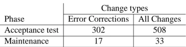
Change types
Phase Error Corrections All Changes
Acceptance test 302 508
Maintenance 17 33
Table 1: Data points according to category
2.2
Available data
Although we would like to assume that all changes are similar in size, this may not be so for enhance-ments, which range from trivial to extensive. How-ever, we can assume similarity in the size of changes for error corrections.
Table 1 shows the count of data points from the ac-ceptance test and maintenance phases (error correc-tions are a subset of all changes). Although our orig-inal goal was to focus on maintenance changes, the limited data encouraged us to include acceptance-test changes. However, interpretation of that data is difficult owing to the different environments, as dis-cussed in Section 4.
2.3
Analysis and threats to validity
The study tests our hypotheses by checking for re-lationships between the independent variables con-cerning software design complexity and the depen-dent variables concerning change isolation effort, change implementation effort, and number of mod-ules changed. The appropriate statistical approach for univariate analysis is a correlation analysis. As will be explained in Section 3, both the isolation and implementation effort metrics lie on an ordinal scale, so we must use a correlation technique which does not require ratio or interval-scale data. We planned to compute Spearman rank-correlation coefficients with respect to single complexity measures of the modules and the maintainability measures.
Based on the notion that a combination of inde-pendent variables might better explain high change effort than only a single variable, we planned to analyze multiple variables in combination using a machine-learning technique called Optimized Set Reduction (OSR) [BTH93, BBH93]. OSR finds patterns in the independent (explanatory) variables which reliably predict values of a single dependent variable. The OSR approach is insensitive to the scale of the data, but requires a large data set, ide-ally several hundred points. We planned to apply the OSR technique to the full data vectors; i.e., consider all explanatory variables together.
If we can find strong correlations between de-sign complexity values and change effort values, or can find patterns of large design complexity values that reliably predict which modules are expensive to change, we will have confirmed our hypotheses for this data set.
There were at least two threats to internal valid-ity. First, the nature of a case study meant that we were not able to control or even measure the factors that influenced the SEL personnel during their day-to-day activities. Second, individual differences may be responsible for some variation (i.e., noise) in the data.
One significant threat to external validity is the specialization of the software-system design used by the SEL. These results may not be applicable to other
FORTRAN systems.
3
Complexity and Maintainability
Curtis refines the concept of software ity into algorithmic and psychological complex-ity [Cur80]. Algorithmic (or computational) com-plexity characterizes the run-time performance of an algorithm. Psychological complexity affects the per-formance of programmers trying to understand or
modify a code module. We measured two aspects of psychological complexity, namely the vertical design complexity (the relationship between specifications and modules) and the horizontal design complexity (the relationship between modules). A module is a file with a single subroutine. These relationships are illustrated in Figure 2. g mod z Spec S1 imple-ments mod x mod y Horizontal complexity Vertical complexity writes read by calls
Figure 2: Vertical and horizontal design complexity
3.1
Vertical complexity:
the relationship
between specifications and modules
The vertical complexity of a modulex is thenum-ber of specifications the module helps implement. To measure vertical complexity, we count how many specifications a module implements directly (men-tioned in the documentation) or indirectly (invoked by another module that implements the specification directly or indirectly). An example is shown in Fig-ure 2, where modulexhelps implement specification
S1 directly and calls moduley, meaning that module yhelps implement S1 indirectly.
3.2
Horizontal complexity: the relationship
between modules
The horizontal complexity of a modulex is
module and other modules. An example is shown in Figure 2, where moduley writes data into a global
variableg, that is read in turn by modulez. We
ana-lyzed the source code to gather data for the following metrics:
Number of COMMON blocks which are
refer-enced in a module.
Number of visible global variables; i.e., the
variables defined in the referenced COMMON blocks.
Number of used global variables; i.e., the
vis-ible global variables that were also used in the code.
Ratio of used global variables to visible global
variables.
For modules p andq, and a variable x within
the static scope of both p and q, a potential
data binding is defined as an ordered triple
(p;q;x)[HB85].
Again usingp,q, andx, a used data binding is a
potential data binding wherepandqeither read
a value from or assign a value tox[HB85].
The fan-in measure of a module is the number
of other modules which call the module.
The fan-out measure of a module is the number
of other modules which the module calls.
3.3
Maintainability
Maintainability is an abstract concept that cannot be assessed directly but may be defined using attributes of the software that can be measured. We use change effort as our metric for maintainability.
Changes. The SEL distinguishes between three types of changes. An error correction repairs faults in the software. An enhancement implements changes for extended specifications. An adaptation makes provisions for alterations in the system’s en-vironment. For us, the error corrections were of pri-mary interest.
Effort data. The analyses presented here are based on a four-step model of the change activity that guides data collection. In step one, the develop-ers/maintainers become aware of the need for a change. Step two involves isolating the modules to be changed. In step three, they plan and implement the change. Finally, in step four they test the changed code. The change effort data that was available to us were limited to the following, routinely collected items [Nat91b]:
Isolation effort: the effort to determine which
modules must be changed (step two).
Implementation effort: the effort to plan,
imple-ment, and test the change (steps three and four)
Locality: the number of components affected
by a change.
Effort expended during the maintenance phase is collected as a point on an ordinal scale, namely “less than one hour,” “one hour to one day,” “one day to one week,” “one week to one month,” and “greater than one month.” Effort expended during the accep-tance test phase is collected using the ordinal scale of “less than one hour,” “one hour to one day,” “one day to three days,” and “more than three days.”
4
Context of the Study
The study was conducted on two projects developed by the Flight Dynamics Division (FDD) of NASA’s
Goddard Space Flight Center. Data about the FDD’s projects are gathered by the Software Engineering Laboratory (SEL), a cooperative effort of NASA’s FDD, Computer Sciences Corporation, and the Uni-versity of Maryland. The SEL was founded and be-gan collecting data about the FDD’s development ac-tivities in 1976. Data collection from maintenance activities began in 1988 [RUV92].
4.1
FDD Staff
The staff who performed the changes were famil-iar with both the application domain (ground-support software for satellites), which were similar for both systems, and the solution domain (FORTRAN), which was identical for both systems.
4.2
Activities in the acceptance test phase
During the acceptance test phase, the original devel-opers exercise the system to detect failures and repair faults as needed [Nat91a]. Enhancements and adap-tations may also be made to the software during this phase owing to new requirements.4.3
Activities in the maintenance phase
During the maintenance phase, a team of software engineers who were not the original developers tests the software using simulators and modifies the sys-tems as needed [Nat91a]. These engineers are ex-perts in their application domain, but not necessar-ily highly familiar with the software systems. The maintenance phase essentially ends when satellites are launched; in any case, no data are collected fol-lowing the launch.4.4
The software systems
Project 1 and Project 2 (names have been changed) are ground-support software systems that were coded
in FORTRAN. Both were single-mission systems.1 Their sizes were approximately 130 and 180 KSLOC (carriage returns). These systems determine the ex-act position of a satellite with respect to other plane-tary bodies using data sent by the satellite. The sys-tems do not run continuously, they are not subject to real-time constraints, and they are not required to meet highly stringent reliability requirements. For both projects, the software architecture and docu-ment standards are highly similar and specific to the FDD environment.
4.4.1 Specifics of Project 1
Project 1 consists of 582 modules. Of those, 23 mod-ules are assembler modmod-ules, with a range of 6–3100 SLOC (carriage returns). The other 559 modules are
FORTRAN modules (range 2–3200 SLOC). The
sys-tem consists of 15 subsyssys-tems.
Changes in acceptance test. The developers pro-cessed 179 change requests during acceptance test-ing. Those change requests directly affected 163 unique modules, but owing to multiple changes to the same modules, there were 306 changes to code modules. Of the 163 changed modules, 32 modules were not available to us, or were assembler modules that were not analyzed. Therefore 48 changes to in-dividual modules and 33 change requests total could not be analyzed.
Project 1 was in development (design, code, and test activities) for approximately 28 calendar months. Of those 28 months, the acceptance test phase lasted approximately 5 months.
1A single-mission system is expected to cost 2% of
de-velopment costs per year in maintenance until it is taken out of service, while a multi-mission system is expected to cost 10% [PS93].
Changes in maintenance. The single maintainer processed 15 change requests during maintenance. Of those, 5 were corrections, 9 were enhancements and 1 was an adaptation. Those change requests di-rectly affected 28 unique modules, but because of multiple changes to the same modules, there were 37 changes to code modules. The assembler modules were not considered (5 change requests, 2 modules). The maintenance phase for Project 1 began in 1988. Because of launch delays, it lasted about 33 months. The level of effort was extremely low for much of that time.
4.4.2 Specifics of Project 2
Project 2 consists of 816 modules. Of those, 31 mod-ules are assembler modmod-ules (range 6–7300 SLOC). In addition to the 747FORTRAN modules (range 3–
2800 SLOC), there are 38 data files (range 9–400 SLOC). The system consists of 30 subsystems.
Changes in acceptance test. The developers pro-cessed 413 change requests during acceptance test-ing. Those change requests directly affected 346 unique modules, but because of multiple changes to the same modules, there were 850 changes to code modules. Of the 346 changed modules, 119 modules were not available to us, or were assembler modules which were not analyzed. Therefore 238 changes to individual modules and 136 change requests total could not be analyzed.
Project 2 was also in development for approxi-mately 28 calendar months. Of those 28 months, the acceptance test phase lasted approximately 7 months.
Changes in maintenance. The four maintainers processed 25 change requests during maintenance. Of those, 12 were corrections, 12 were enhance-ments, and 1 was an adaptation. Those change
requests directly affected 55 unique modules, but because of multiple changes to the same modules, there were 67 changes to code modules. Fortunately for our analysis, the assembler modules were not changed.
The maintenance phase for Project 2 began in 1988 and lasted about 19 months.
5
Results
After discussing some problems with the data, we present results from analyzing the maintenance and acceptance test data and sketch results from related work.
5.1
Data difficulties
We encountered some difficulties while trying to col-lect the data for the metrics defined in Section 2. In all fairness to the SEL, their data-collection forms were not designed to support such a detailed investi-gation, and we could not change data collection after the fact, so some problems were to be expected.
First, collecting data for metric M1 depended both on the modularity of the specification and the trace-ability of the specification to the code. At one ex-treme of modularity, the whole project can be seen as one single specification, while at the other extreme, every condition such as “x ¿ 0” can be also seen as a specification. We began by using the system de-scription document, in which a system is divided into 40–70 subspecifications. Even with this coarse level of modularity, it was not possible to map the mod-ules to the subspecifications with any hope of accu-racy because there was no document containing this information. We resolved this difficulty by simplify-ing the problem. Because the subsystems (Projects 1 and 2 had 15 and 30, respectively) were easily iden-tifiable both in the requirements document and in the
code, we essentially labeled each subsystem a “spec-ification.” Then we traced modules back to subsys-tems by analyzing the calling structure of the code.
The change effort data presented a second prob-lem. In the SEL environment, a change activity oc-curs in response to a change request, and may affect many modules. The effort data are collected for each change activity, but no data for the change effort per
module are collected. Because it is impossible to
de-termine from the data how much change effort was expended on individual modules, we could not ob-tain values for metrics M10, M11, and M12 as orig-inally planned. We resolved this difficulty by using an average for each change, namely the average of the complexity measures that were collected from the modules affected by that change. All analyses therefore are focused on changes rather than mod-ules. However, by averaging, we reduced the range in complexity values, possibly losing significant dif-ferences.
Finally, we concluded that significant differences in effort were hidden by the ordinal scale of the ef-fort data. For example, a maintenance change that required 9 hours of implementation effort is quite different from one that required 39 hours, but both are classified identically as “one day to one week.”
5.2
Results from the maintenance data
5.2.1 Vertical complexity measures
First we tested hypothesis 1 using maintenance data, subject to the caveats discussed in Section 5.1.
Data collection process. We built a prototype tool that extracted the module calling trees from theFOR
-TRAN code for each subsystem. This information told us which modules were part of a particular sub-system. While collecting these data, we found that not all of the modules changed are executable
mod-ules, and therefore are not in the call tree. Mea-sures of change effort were obtained by querying the SEL database [Nat90] and by examining the data-collection forms completed by the maintainers after making the changes.
Results from univariate analyses. For Project 1, 19 modules that were changed were found in the call tree. Of those 19 executable modules, only 3 sup-ported multiple subsystems; i.e., helped implement more than one specification. For Project 2, 32 mod-ules that were changed were found in the call tree. Of those 32 executable modules, only 1 supported mul-tiple subsystems. This left us with 4 data points for changed modules which supported multiple subsys-tems. None of the 4 modules participated in changes with above-average isolation or implementation ef-fort.
Results from multivariate analyses. The OSR technique requires a large set of data to be effective. Because the maintenance data set was too small to be used, we have no multivariate results.
Interpretation. We could not support hypothe-sis 1; the answer to questions 2.1, 2.3, and 2.5 was “not for these data.” Although our analysis found many modules that supported more than one sub-system, few of those modules were changed. We later learned that many of the modules which are widely reused are utility functions or so-called “insti-tutional software.” This term refers to modules that are reused repeatedly from project to project and are rarely changed.
We also learned that subsystems are designed mostly in isolation from one another, with the re-sult that modules are not reused widely across sub-systems. Although our definition of a “specifica-tion” was arguably too coarse, we could not refine
the traceability further without a detailed familiarity with the systems.
An interesting result was that for Project 1, 12 of the 19 changed executable modules were from a sin-gle subsystem. No comparable, frequently changed subsystem was identified in Project 2, although the changes were clustered in 5 of the 30 subsystems.
5.2.2 Horizontal complexity measures
Next we tested hypothesis 2 using maintenance data.
Data collection process. We built a prototype tool which counted the use of common blocks and common-block variables in the FORTRAN code, and
reused the calling-tree information from the analy-sis of vertical complexity for the measures of fan-in and fan-out. After loading all the resulting data into a database system, it computed the necessary com-plexity values. Recall that module comcom-plexity values were averaged on a per change basis as explained in Section 5.1. Effort data were obtained as discussed in Section 5.2.1.
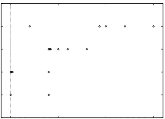
Results from univariate analyses. Figure 3 uses data about error corrections from the maintenance phase to plot isolation effort against the average number of used common blocks (metric M2) in the modules affected by each change. This figure shows a trend towards higher effort when the average num-ber of common blocks is also high. Thus encour-aged, we computed correlations for the change data from the maintenance phase.
Table 2 shows the Spearman rank-correlation co-efficient values for the relationships between all in-dependent and in-dependent variables for all changes during maintenance; Table 3 shows only the coeffi-cient values for error corrections. The correlations were computed as explained in Section 2.3. An ap-proximation of the .05 cutoff (a 5% chance of
obtain-0 1 2 3 4 5 0 5 10 15 Isolation effort
Average number of common blocks
Figure 3: Data for error corrections in maintenance
ing the numbers by chance) is given in both tables to help judge the significance of the results.
Results from multivariate analyses. As men-tioned previously, we had too few data points to ap-ply OSR to the maintenance data.
Interpretation. When considering all changes during maintenance, all measures of global variables correlated positively (some significantly) with isola-tion effort. The counts of used globals and actual data bindings showed the most significant correla-tion of all measures; in an absolute sense the corre-lation is weak (approximately 0.60). These results support the idea that global variables make a pro-gram difficult to understand, although this conjecture was not supported by [LZ84] (see also Section 5.4). We found no significant correlation between com-plexity measures and implementation effort, nor be-tween complexity measures and the number of mod-ules changed. The measures of control-flow com-plexity were not helpful. To summarize the results for all changes, we can support hypothesis 2 in some
Independent variables
Dependent variables Isolation Implem’n Modules
(averages per change) effort effort changed
M2: Common blocks .415 .088 -.376
M3: Visible global vars .575 .207 -.303
M4: Used globals vars .628 .228 -.198
M5: Ratio used:visible globals .534 .303 .105
M6: Potential data bindings .528 .193 -.330
M7: Used data bindings .599 .214 -.294
M8: Fan-in -.268 -.010 .067
M9: Fan-out .322 .181 -.363
N = 33, critical r (.05) t approximation = .343
Table 2: Spearman rank-correlation coefficients for all changes during maintenance
Independent variables
Dependent variables Isolation Implem’n Modules
(averages per change) effort effort changed
M2: Common blocks .738 .403 -.169
M3: Visible global vars .785 .511 -.143
M4: Used global vars .799 .511 .000
M5: Ratio used:visible globals .619 .493 .164
M6: Potential data bindings .770 .511 -.214
M7: Used data bindings .813 .511 -.102
M8: Fan-in -.406 -.208 -.096
M9: Fan-out .610 .545 -.143
N = 17, critical r (.05) t approximation = .482
respects; the answer to question 2.2 (isolation effort) is a qualified yes for some of the measures, but the answer to questions 2.4 (implementation effort) and 2.6 (locality) is “not for these data.”
When considering just the error corrections during maintenance, the measures of global variables cor-relate positively and much more strongly with the isolation effort than previously. Both the counts of used globals and actual data bindings again showed the most significant correlations, in this case fairly strong in an absolute sense (approximately 0.80). We also found correlations with implementation effort; some were significant but again weak in an absolute sense (approximately 0.50). Fan-out correlated posi-tively weakly with both measures of effort. No mea-sures correlated with the number of affected mod-ules. To summarize the results for the error correc-tions, we can support hypothesis 2 strongly; the an-swers to questions 2.2, 2.4, and 2.6 are a reasonable yes, a weak yes, and another “not for these data.”
Finally, we found it interesting that the number of changed modules frequently correlated negatively, although weakly, with the complexity values. We are unable to explain this result.
5.3
Results from the acceptance test data
As mentioned earlier, we extended the scope of the study to include data from the acceptance test phase. The results must be interpreted carefully, because the measures of the source code were computed using the code as it existed at the end of the maintenance phase. A version of the code from the end of the acceptance test phase was not available.5.3.1 Vertical complexity measures
Due to the problems discussed in Sections 5.1 and 5.2.1, we did not test hypothesis 1 using accep-tance test data.
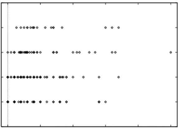
0 1 2 3 4 5 0 5 10 15 20 25 Isolation effort
Average number of common blocks
Figure 4: Data for error corrections in acceptance test
5.3.2 Horizontal complexity measures
Finally, we tested hypothesis 2 using the acceptance test data.
Data collection process. The measures M2 to M9 were computed from the source code as of the end of the maintenance phase. Again, module complexity values were averaged on a per change basis as explained in Section 5.1. Measures of change effort were obtained by querying the SEL database [Nat90].
Results of univariate analyses. Figure 4 uses data about error corrections from the acceptance test phase to plot the isolation effort against the average number of common blocks in the modules affected by each change. Plots of isolation and implementa-tion effort against other independent variables were similarly random, which discouraged us from com-puting univariate correlations.
Results of multivariate analyses. Because we had data for several hundred changes in the acceptance test phase, we were able to apply the OSR tech-nique [BTH93, BBH93]. Based on the results achieved when working with the maintenance data, we restricted the data set to the error corrections. All analyses took the approach of trying to iden-tify whether the error corrections (changes) would be inexpensive or expensive, where inexpensive was defined as requiring one day or less (the lower two values on the ordinal scale) and expensive was de-fined as requiring more than one day (the upper two values). The technique found reliable patterns when using isolation effort as the dependent variable, but found no reliable results when using implementation effort or locality as the dependent variable.
All results are expressed as OSR patterns. Pat-terns provide interpretable models where the impact of each predicate can be easily evaluated [BTH93]. An OSR pattern is a set of one or more predicates, where predicates have the form (EVi
2EVclass ij),
meaning that a particular explanatory (independent) variable EVibelongs to part of its value domain, i.e.,
EVclassij. Taken as a whole, the pattern predicts
whether the value of the dependent variable will be in the high-cost or the low-cost class. For each pattern, we state the reliability of the prediction (a measure of pattern accuracy), and the significance level of the reliability (whether the pattern is based on a suffi-ciently large set of data to be trusted). The OSR tech-nique found reliable and significant patterns which predict low and high isolation effort. We present pat-terns which had high reliability values (¿ 0.8) and low reliability significance values (¡ 0.05).
Pattern L1:
Fan-in226-100% AND
fan-out20-50%)low
(reliability 0.85, rel. sig. 0.011)
Pattern L1 suggests that modules with medium to
high fan-in values and low fan-out values were easy to change (predicts low isolation effort). This pattern may indicate leaf modules (such as library subrou-tines) which are called frequently but call few other modules.
Pattern L2:
Used var20-12% OR
used db20-11%)low
(reliability 0.92, rel. sig. 0.001)
Pattern L2 suggests that modules with low num-bers of used variables or low numnum-bers of used data bindings were easy to change (predicts low isolation effort).
Pattern H1:
Fan-in28-26% AND
(used db220-100% OR
used var220-100%))high
(reliability 1.00, rel. sig. 0.000)
Pattern H1 suggests that if a module is called by a relatively low number of other modules, and addi-tionally has many used data bindings or many used variables, then that module was expensive to change (predicts high isolation effort).
Pattern H2:
Ratio used:visible263-100% AND
(vis var234-100% OR
used db230-100%))high
(reliability 1.00, rel. sig. 0.001)
Pattern H2 suggests that if a module has a high ra-tio of used to visible global variables, and addira-tion- addition-ally has many visible variables or many used data bindings, then that module was expensive to change (predicts high isolation effort).
Pattern H3:
Fan-out242–100%
AND used db259-100%)high
(reliability 1.00, rel. sig. 0.007)
Pattern H3 suggests that modules which call many other modules and have many data bindings to other modules were expensive to change (predicts high isolation effort).
Interpretation. The univariate analyses were not helpful, but the OSR analysis identified some pat-terns that reliably characterize modules which par-ticipated in error corrections with both low and high isolation effort. All of the patterns support hypothe-sis 2. We have not established a causal relationship between the patterns and isolation effort, no statisti-cal analysis technique does so, but we have identified a set of patterns that may be suitable for further in-vestigation.
5.4
Results from related studies
We summarize the results of previous studies and ex-periments that analyzed the effects of design com-plexity on various dependent variables. Note that comparisons with related work are dangerous owing to different definitions of both independent and de-pendent variables.
Lohse and Zweben [LZ84] ran a controlled exper-iment to examine the effects of data coupling (data flow among modules) via global variables versus for-mal parameters, in the context of performing mainte-nance changes (enhancements) to two software sys-tems. The primary dependent variable was the time required to implement the enhancement. They found no significant differences attributable to the use of global variables versus formal parameters.
Card et al. [CCA86] performed a case study on five SEL FORTRAN systems to examine the impact
of various design practices on the dependent vari-ables fault rate and cost in the context of develop-ment. They found no correlation with the percentage of referenced variables in COMMON blocks but a positive correlation with the number of descendants (fan-out). The percentage of unreferenced variables from COMMON blocks correlated with faults, but not with cost.
Rombach [Rom87] ran a controlled experiment to examine the effects of various programming-language constructs on isolation effort, implementa-tion effort, and locality in the context of performing maintenance changes (enhancements) to two soft-ware systems. Complexity was measured in terms of information flow, which includes both data bind-ings and control flow between modules. He found a correlation of both isolation effort and locality with external complexity, but no correlation of implemen-tation effort with external complexity. Our results support his with respect to isolation and implemen-tation effort, but not locality.
Card and Agresti [CA88] performed a case study on SELFORTRAN systems to test for a relationship
between a combined complexity measure and either productivity (lines of code delivered per unit of time) or fault rate in the context of development. Their combined measure of local complexity (e.g., cyclo-matic complexity) and structural complexity (e.g., module fan-out) correlated well with productivity and number of faults. Because their study does not separate local (internal) complexity from structural (external) complexity, we cannot compare results.
6
Conclusion and Lessons Learned
The data from the two SEL systems support our hy-pothesis 2, so we can answer in the affirmative that horizontal design complexity appears to affect main-tenance effort (isolation effort for error corrections).
However, we have only demonstrated a possible rela-tionship. We cannot establish causation using a case study.
Next we summarize the results of the study in terms of what the SEL can learn, what we learned, and what the software-engineering community can learn. Our analyses, which we primarily see as point-ers for further investigation, found a number of re-lationships between software design complexity and maintenance effort that might help the SEL predict maintenance effort. Univariate analysis showed that the metrics “used globals” and “used data bindings” correlated strongly with the isolation effort for er-ror corrections performed during the maintenance phase. Data for other metrics relating to the defini-tion and use of global variables also correlated with isolation effort, but much less strongly with imple-mentation effort. The measure of fan-out was also somewhat helpful in explaining high isolation effort. Multivariate analysis of acceptance test data using OSR found a number of patterns which were strong indicators of both low and high isolation effort in this data set. Future studies could be performed using other SEL systems to test whether the relationships and patterns which we found hold for more than just the two systems that we analyzed.
We gained a better understanding of the data re-quired for thoroughly testing our hypotheses. First, to measure vertical complexity, both the modularity of the specification and its traceability to the code must be addressed. To solve the latter problem, a traceability matrix could be constructed in which the rows represent individual code modules and the columns represent units of the specification. A mark in the matrix means that the module of that row im-plements the unit of specification of that column. To build such a matrix, the modularity of the specifica-tion is critical, but beyond the scope of this paper. Second, to measure the effort required for a change, we need to collect the isolation and
implementa-tion effort on a per-module basis whenever possible. A minor change to the SEL’s data-collection forms could be to collect an estimate of the percentage of the total effort required by each module. However, some effort, such as the effort to test the changed modules together, cannot be allocated to individ-ual modules. Third, the simplest and most helpful change to the SEL’s data collection forms (from our point of view) would be the use of a ratio scale such as days or hours for collecting effort data instead of the ordinal scales currently in use. This would al-low us to distinguish more precisely between differ-ent changes as well as to compare effort data between the maintenance and acceptance test phases.
Finally, we believe that an empirical investigation such as this one uncovers more challenging ques-tions than it answers. Future work might include replicating our study by analyzing the designs of other SEL software systems or systems from other software development organizations. Our data might also be used as a basis for planning and running a controlled experiment such as the one discussed in [Rom87] to test our hypotheses more rigorously. In a controlled experiment, programmers (subjects) might implement changes of similar sizes in mod-ules that have low, medium, and high software de-sign complexities. This would allow the researchers to control for many effects as well as to measure the effort required on a per-module basis to implement changes. Such an experiment would offer stronger evidence for refuting or accepting our hypotheses than any case study.
7
Acknowledgements
We would like to thank Lionel Briand and Alfred Br¨ockers for help with the analyses, Dieter Rombach for suggesting the hypotheses, Jon Valett for answer-ing our questions, and most importantly, the SEL for
trusting us with their systems and data.
References
[BBH93] Lionel C. Briand, Victor R. Basili, and Christopher J. Hetmanski. Developing interpretable models with optimized set reduction for identifying high-risk soft-ware components. IEEE Transactions on
Software Engineering, 19(11):1028–1044,
November 1993.
[BR88] Victor R. Basili and H. Dieter Rom-bach. The TAME Project: Towards improvement–oriented software environ-ments. IEEE Transactions on Software Engineering, SE-14(6):758–773, June 1988.
[BTH93] Lionel C. Briand, William M. Thomas, and Christopher J. Hetmanski. Modeling and managing risk early in software devel-opment. In Proceedings of the Fifteenth
International Conference on Software En-gineering, pages 55–65. IEEE, May 1993.
[BW84] Victor R. Basili and David M. Weiss. A methodology for collecting valid software engineering data. IEEE Transactions on
Software Engineering, SE-10(6):728–738,
November 1984.
[CA88] David N. Card and William W. Agresti. Measuring software design complexity.
Journal of Systems and Software, pages
185–197, June 1988.
[CCA86] David N. Card, Victor E. Church, and William W. Agresti. An empirical study of software design practices. IEEE
Trans-actions on Software Engineering,
SE-12(2):264–271, February 1986.
[Cur80] Bill Curtis. Measurement and experi-mentation in software engineering.
Pro-ceedings of the IEEE, 68(9):1144–1157,
September 1980.
[Epp94] Andreas Epping. An empirical investi-gation of the impact of the structure of two software systems on their maintain-ability (in German). Master’s thesis, De-partment of Computer Science, University of Kaiserslautern, 67653 Kaiserslautern, Germany, April 1994.
[HB85] David H. Hutchens and Victor R. Basili. System structure analysis: clustering with data bindings. IEEE Transactions on Software Engineering, SE-11(8):749–757,
August 1985.
[LZ84] John B. Lohse and Stuart H. Zweben. Ex-perimental evaluation of software design principles: An investigation into the ef-fect of module coupling on system modi-fiability. Journal of Systems and Software, 4(4):301–308, November 1984.
[Nat90] National Aeronautics and Space Adminis-tration. Software Engineering Laboratory (SEL) Database Organization and User’s Guide, Revision 1. Technical Report SEl-89-101, NASA Goddard Space Flight Center, Greenbelt MD 20771, February 1990.
[Nat91a] National Aeronautics and Space Adminis-tration. Manager’s handbook for software development. Technical Report SEL-84-101, NASA Goddard Space Flight Center, Greenbelt MD 20771, 1991.
[Nat91b] National Aeronautics and Space Adminis-tration. Software engineering laboratory
(SEL) relationships, models, and manage-ment rules. Technical Report SEL-91-001, NASA Goddard Space Flight Center, Greenbelt MD 20771, February 1991. [PS93] Rose Pajerski and Donald Smith. Recent
SEL experiments and studies. In
Pro-ceedings of the Eighteenth Annual Soft-ware Engineering Workshop, pages 81–
94. NASA Goddard Space Flight Center, Greenbelt MD 20771, 1993.
[Rom87] H. Dieter Rombach. A controlled exper-iment on the impact of software structure on maintainability. IEEE Transactions on
Software Engineering, SE-13(3):344–354,
March 1987.
[RUV92] H. Dieter Rombach, Bradford T. Ulery, and Jon Valett. Toward full life cycle con-trol: Adding maintenance measurement to the SEL. Journal of Systems and Software, 18(2):125–138, May 1992.