Multi-objective analysis of machine learning algorithms using model-based optimization techniques

(1)

fakultät

statistik

Multi-objective Analysis of Machine Learning Algorithms

Using Model-based Optimization Techniques

Dissertation

by

M.Sc. Data Science DANIELHORN

in partial fulﬁllment of the requirements for the degree of

Doktor der Naturwissenschaften

Submitted: Dortmund, January 2019 Primary referee: Prof. Dr. Claus Weihs Secondary referee: JProf. Dr. Andreas Groll Commission chairperson: Prof. Dr. Jörg Rahnenführer

Assessor: Dr. Michel Lang Day of the oral examination: 20th February 2019

(2)

(3)

Preambel

This dissertation summarizes my work during the last ﬁve years, from October 2013 to December 2018 and covers all of my publications originating from this period. Since it is cumulative, only brief summaries of the contributed articles are given. Exhaustive results are mostly omitted and the original articles are referred instead. This text arranges the publications into the big picture and gives introductions to their respective research ﬁelds, starting from the absolute basics. For more in-depth details I recommend to read the respective articles themselves. Apart from the introduction and the conclusion, each chapter of this work concludes with a section on the con-tributed material. After a simple enumeration of the concon-tributed papers and software libraries, a short description on how they arose follows.

Since this dissertation covers the fields of optimization, machine learning and algorithm se-lection, it was not possible to use a consistent notation throughout all chapters. Notation is only locally valid and can change when advancing to another research field. However, I tried to use some letters consistently during the entire work. X always corresponds to an influential parame-ter, whileY corresponds to a target variable and f to the functional connection betweenX andY. Variations of these are used to describe the observations and parameter spaces. Table 1 gives an overview to this notation and can be used as an look-up table.

This work would not have been possible without the help of many people. At ﬁrst, I want to thank Prof. Claus Weihs. I still remember this afternoon in January in 2013. I was about to start working on my master thesis and just made up my mind that I would like to stay at the university afterwards as an Ph.D. student. After his lecture in the course classiﬁcation methods, I told him

X(i) i-th inﬂuential parameter Y/Y(i) (i-th) target variable

X parameter space Y objective space

X(i) _{space of the}_i_{-th parameter} _Y(i) _{space of the}_i_{-th objective}

xxx observation vector y/yyy corresponding target value(s)

xxxj optional numbering ofxxx yj/yyyj optional numbering ofy/yyy

x(i) observation of thei-th parameter y(i) observation of thei-th objective

f:X →Y functional relation of theX(i)andY fˆ estimator / model for f

Table 1: Notation used consistently through the entire work.

(4)

about my decision and asked if I could start working at his chair. He just answered with the counterquestion: "Okay, when would you like to start?", and afterwards I was employed. Claus Weihs had trust in my competence and gave me the opportunity to follow my own ideas from the ﬁrst day on. I am very grateful for this.

At second, I want to thank Bernd Bischl. Although Claus Weihs is the official supervisor of my dissertation, Bernd surely was my mentor, at least during its first years. Most of the things I have learned during the last year of my master’s degree and in the first years of my graduation, I have learned from or because of Bernd. Since he left to Munich halfway through my graduation, it was complicated to continue the good collaboration in the subsequent years. Nevertheless, without Bernd many of the contributed work would not have been possible.

Moreover, I have to thank all remaining co-authors of my contributed publications. Tobias Wagner, especially for introducing me to many people in the multi-objective optimization com-munity. Aydın Demircio˘glu and Tobias Glasmacher for their support in the project SVMs for large data sets. Jakob Richter, Jakob Bossek, Janek Thomas and Michel Lang as the remaining members of themlrMBOteam. Martin Zaefferer for his work on hierarchical Kriging kernel, who had a hard time remotivating me after some ﬁrst frustrating results. My student workers Karin Schork and Rosa Pink, who supported me in many ways. Swetlana Herbrandt and Nadja Bauer, as well as the remaining members of the chair for computational statistics, for all the informative discussions during the last ﬁve years. Andreas Groll, for agreeing to co-review this dissertation.

A special thank has to go to Rosa Pink, once again, for proof reading this text. I cannot count the hours we spend on discussing single sentences, even words, until this work was finally finished. Additional thanks go to Claus Weihs, Andreas Groll, Michael Kirchhoff, Jennifer Neuhaus-Stern, Marie-Louise Vosteen and Steffen Maletz for finding many mistakes and giving helpful comments. And, at last, my biggest thank has to go to TU Dortmund university’s faculty of statistics and all the countless students and colleagues I met during the last ten years. You made this place a home and yourselves a family for me.

(5)

Introduction

Data is the sword of the 21st century, those who wield it the samurai.

– Jonathan Rosenberg, former Senior Vice President of Products at Google

This and many other quotes can be heard these days when talking about data and data science. Data is called theoilor even thesoilof the 21st century, data science thesexiestjob. Many com-panies have distinct data science departments and some comcom-panies like Google or Facebook make billions of dollars every year, mainly based on their ability to process large datasets. Nowadays, to collect, analyze and learn from large amounts of data is both a challenge and an opportunity.

At the same time, data science has a relatively young history. The term itself goes back around forty years and has started to be more frequently used in the last decade. Study courses on data science aren’t sprouting more than two or three years ago. However, data has been collected for much longer. The Romans and even earlier cultures performed population censuses and mea-sured other related information, the probably most popular data collection is even mentioned in the Christmas story. Although it has not been called data science, data has been analyzed ever since. At the beginning of the 20th century, the term statistic arose for this scientific field and its mathematical foundations were laid. Data, however, was scarce, and statistic is often focused on making the best out of only a few observations. Today, in the age of the world wide web with companies like Google and Facebook, data is produced at a rapid pace. Ten years ago, in 2008, Google alone processed estimated 20 peta bytes of data per day.1 Hence, data science often suffers from an abundance of available data, rendering most classic statistical methods inappropriate or even inapplicable. Nevertheless, both fields rely on the same foundation: on data.

Most data sets consist of two types of variables. First, there is a set called target variables, here denoted withY. These are the variables one wants to gain new knowledge about. Examples are the quality of a product, the risk of an accident happening or the (monetary) proﬁt. Often, only a single target variable is considered, however, in some situations it is necessary to investigate multiple ones. Second, there is a set called the independent variables, here denoted withX. These

1_{https://www.niallkennedy.com/blog/2008/01/google-mapreduce-stats.html}_{, 09/18/2018}

(8)

variables can be any other property of the unit of observation, as for example the height and the sex of a person, or some diagnostic measures of a workpiece. Moreover,X variables are assumed to have an inﬂuence on theY variables: If the value of anXvariable is changed, it is expected that also the value of the target variables changes, i.e. some kind of relationshipX →Y is assumed.

Although data science and statistics are all about data, it is neither theX nor theY variables one is mostly interested in. Instead, it is the arrow in-between those variables: To understand the relationship between the dependent and the target variables. Typical questions are:

• Interpretation: If a certainXvariable is changed, how will it affect theY variables?

• Prediction: Given values of theXvariables, what values will theY variables take?

• Optimization: Which values of theX variables will result in optimal values of theY variables? Finding good answers to these questions often requires a deep understanding of both, theX and theY variables, as well as of the underlying data generating process.

Most times, these questions demand an important intermediate step: To find a good model describing the relationship between X andY, also known as model selection. Here, not only an adequate model class has to be found, but also its hyperparameters have to be set. Hence, finding a good model is not only an intermediate step in most data analyses, it is also a data analysis itself, where the target variable is defined as the quality of the model and the dependent variables are the choice of the model class and its subsequent hyperparameters. Many data science problems imply solving this internal optimization problem, the optimization of the model quality. Therefore, the main focus of this work lays on optimization. It is organized as follows:

The second chapter gives an introduction into the topic of optimization. At first, an overview over different disciplines within the topic is given and the training of a support vector machine is presented as an exemplary task. Afterwards, the sequential model-based optimization approach for expensive problems and its extensions for multi-objective optimization problems are presented. The third chapter focuses on hyperparameter tuning as a special optimization problem. At first, an introduction to machine learning and the general machine learning scheme is given. Again, the SVM is used as an example, here for tuning its hyperparameters, both in a single- and a multi-objective setting. Tuning as an optimization problem can have difficult properties. It can be both expensive and stochastic, and the parameter space can include mixed and hierarchical parameters. The chapter continues with adapting sequential model-based optimization for these properties.

The fourth chapter discusses algorithm selection. This special data science task deals with the choice of the best algorithm for solving a given problem. Here,Y is the available algorithm, while

X variables include performances of the algorithms on various problems. This work addresses a multi-objective context. In contrast to the single-objective case, here not only a single but a whole set of optimal algorithms has to be selected with respect to multiple contradicting perfor-mance measures. Once again, the SVM is used as an application: Approximate SVM solvers are compared with respect to the objectives training time and missclassiﬁcation error.

(9)

Chapter 2

Optimization

Optimization problems (OPs) occur in many – if not all – practical data analyses. In technical processes it may be the quality of the produced objects, in biometrics the efficacy of a drug, or model qualities in general statistic applications. No matter how diverse these situations are in their details, they do not differ in their main components. All of them feature some kind of process, which is controlled by several parameters. Given a parameter setting, i.e. a specific value for each parameter, the process can be executed and some sort of performance value is returned. The goal is to find parameter settings that result in best performances. This procedure is called optimization, the best setting, corresponding to an optimal performance, is called the optimum.

Mathematically, the underlying process can be described by a function f :X →R, where

X =X(1)_×_X(2)_×_..._×_X(d)_{denotes the set of all feasible parameter settings. For a speciﬁc} parameter settingxxx= [x(1)_,_x(2)_,...,_x(d)_]T_∈_X_{, where}_x(i)_∈_X(i)_{is the value of parameter}_X(i)_, the associated ﬁtness value is denoted by f(xxx). Since maximizing f is equivalent to minimizing

−f, only minimization problems are considered here. The (global) minimum of f is deﬁned as the set of all solutions fulﬁlling

min

xxx_∈_X f(xxx):={xxx∈X|xxx˜˜˜∈X : f(xxx˜˜˜)< f(xxx)}.

The class of all OPs contains an incredible amount of rather distinct problems. Therefore, the existence of a global optimization strategy, working quite well for every OP, is pretty unlikely. An algorithm that performs reasonably well for many OPs is the most simple one: random search. Random search (RS) iteratively draws uniformly distributed settings fromX and evaluates them with funtil some kind of termination criterion is reached, usually a predeﬁned budget. Finally the setting with minimal target value is considered as the optimum.

It has actually been proven by Wolpert and Macready (1997) that all optimization algorithms have the same expected performance as random search if the OP is chosen uniformly from all possible OPs. This behavior is known as theno free lunch theorem(NFL). However, it is a merely theoretic result and, in practice, algorithms do perform better than RS. Random search’s most important advantage is also a huge disadvantage: It incorporates (almost) no application speciﬁc knowledge. Hence, if meta-information about a speciﬁc subclass of OPs is available, a reasonable

(10)

algorithm using this information should give better results than RS. This is not in contradiction with the NFL, since now the OP is not chosen from a uniform distribution of all possible OPs, but comes from a smaller subclass.

One example is the subclass of purely continuous OPs. In this subclass, the parameter space

X(i)_{of each parameter}_X(i)_{is given by an interval}_x(i) le f t;x

(i) right

. If it can also be assumed that f

is convex and if the analytical form of its derivative is known, Quasi-Newton algorithms and espe-cially the BFGS method (simultaneously published by Broyden, Fletcher, Goldfarb and Shanno in 1970) have shown to be very effective.1 Another example is the pure discrete setting. Here, each parameter Xi can only take a ﬁnite number of different values. If the cardinality ofX is small enough, every parameter setting can be evaluated with f and, consequently, the global optimum of f will be found.

In both examples, X is described by so-called box-constraints and no further restrictions are given. Such OPs are called unconstrained. Though, in many practical applications further restrictions on X do exist. For example, X can be confined by constraint functions gand h. A setting xxx is only feasible if both g(xxx)≥0 and h(xxx) =0 hold. In section 2.1 an exemplary constraint OP is presented. As a second example, hierarchical parameter structures can exist. A hierarchical parameter X(i) _{is only active (i.e., has an influence on} _f_{) if other parameters fulfill} certain conditions. Instances of such OPs are given in chapter 3. Further restrictions onX may be possible, but are not investigated here.

In the ﬁrst example subclass, some major information on the structure of f is given: f is convex. However, in many practical OPs the structure of f is mostly unknown, aside from the pa-rameter spaceX. This class of OPs is referred to as blackbox OPs. It can be further distinguished between pure continuous settings, where all parameters are continuous, and mixed settings, where both continuous and discrete parameter do exist. Both, continuous and mixed blackbox OPs are addressed later in this work.

State-of-the-art approaches for solving continuous blackbox OPs include evolutionary strate-gies2(ESs). Especially the Covariance Matrix Adaption ES (CMA-ES) by Hansen et al. (2003) shows on-top performances in many ongoing benchmarks, for example in the blackbox optimiza-tion benchmarks by Hansen et al. (2016). However, ESs require (hundreds of) thousands of func-tion evaluafunc-tions until they converge towards the global optimum. This is infeasible for many applications due to possible high costs of single evaluations. Here, the term cost mostly refers to the time a single evaluation takes, but can also be interpreted in other application dependent ways as its monetary costs. Such OPs are referred to as expensive OPs.

In recent years, a class of algorithms for solving expensive OPs has been developed. Based on the efﬁcient global optimization (EGO) procedure by Jones et al. (1998), their main idea is

1_{See, e.g., Weihs et al. (2013) for an introduction to Quasi-Newton methods.} 2_{See, e.g., Yu and Gen (2015) for an introduction to evolutionary strategies.}

(11)

EXAMPLE: SUPPORT VECTOR MACHINES 5

to replace f by an inexpensive surrogate function ˆf. In order to estimate ˆf, some evaluations have to be performed with f itself. These so called sequential model-based optimization (SMBO) approaches iterate between evaluating f and optimizing ˆf. Parts of this work are focused on extending the general SMBO approach for some special applications.

This chapter continues by introducing the training of support vector machines (SVMs) as a speciﬁc class of OPs as well as a dedicated specialized optimization algorithm. Subsequently, the SMBO approach is explained in its details. For some OPs, not only a single but multiple objectives have to be optimized mutually. These multi-objective OPs are introduced in the last section, along with related extensions for the SMBO procedure.

2.1 Example: Support Vector Machines

The Support Vector Machine (SVM) (Cortes and Vapnik, 1995) is a binary classiﬁcation method. Fornobservations(xxxT

1,...,xxxTn)T ofdcontinuous parameters and a binary labelyi∈Y =:{−1,1} for each observation, the SVM estimates the true, unknown relationship f:X →Y. In its most simple form, the so-called linear hard-margin SVM assumes linearly separable classes. Thus, f is modeled by

ˆ

f(xxx) =sign(βββTxxx−β0),

withβββ ∈Rd andβ0∈Rsuch that yi·(βββTxxxi−β0)≥1 holds for all observations andβββTxxxi−β0

equals−1 and+1 for at least one observation. The lineβββTxxxi−β0=0 is called decision boundary.

Since there is an inﬁnite amount of feasible vectors(β0,βββ), the SVM uses an additional optimality

criterion: the size of the so-calledmargin. It is deﬁned as the distance between the two hyperplanes βββT_xxx₋_β

0=±1. As known from linear algebra, this distance is given by _||_βββ2_||

2, whose maximization

is equivalent to the easier minimization of 1₂||βββ||2₂. Hence, training a linear hard-margin SVM means solving the optimization problem

min β∈Rd 1 2||βββ|| 2 2 subject to yi·(βββTxxxi−β0)≥1 ∀i=1,...,n.

The assumption of linear separable classes is rather unrealistic. Therefore, the soft-margin SVM allows some observationsxxxi to lie inside the margin, i.e. yi·(βββTxxx−β0)∈[0; 1), or even on

the wrong side of the decision boundary, i.e. yi·(βββTxxx−β0)<0. Figure 2.1 shows an exemplary

data situation, including ﬁve observations violating the margin. The former hard constraints are softened by introducing so-calledslack variablesξiand the OP is be extended to optimizing both the size of the margin and the sum of the slack variables. A hyperparameterCis introduced to

(12)

● ● ● ● ● ● ● ● ● ● ● ● ● ● ● ● ●● ● ● ● ● ● ● ● ● ● ● ●● ● ● ● ● ● ● ● ● ● ● ● ● ● ● ● ● ● ● ● ● ● ● ● ● ● ● ● ● ● ● ● ● ● ● X(1) X ( 2 ) βTx− β0=0 βTx− β0= −1 βT_x_{− β} 0=1 ● ● Class −1 Class 1 ξi ξi ξi ξi ξi

Figure 2.1 Example classiﬁcation problem for classes -1 and 1. The solid line corresponds to the decision boundary, the dashed lines visualize the margin.

control the trade-off between those two objectives, resulting in the optimization problem min β∈Rd 1 2||βββ|| 2 2+C n

∑

i₌1 ξi subject to yi(βββTxxxi−β0)≥1−ξi ∀i=1,...,n.

The assumption of a linear decision boundary between the two classes is also quite naive. To handle classiﬁcation problems with non-linear decision boundaries, the SVM utilizes the so-called

kernel-trick: By applying a functionΨthe parameters are transformed into a higher-dimensional feature space, in which the classes are more likely to be linearly separable. Finally, the OP of the non-linear SVM can be formulated as

min β∈Rd 1 2||βββ|| 2 2+C n

∑

i=1 ξi subject to yi(βββTΨ(xxxi)−β0)≥1−ξi ∀i=1,...,n.

According to Bottou and Lin (2007), this so-called primal OP is a quadratic, convex OP and can be solved with appropriate standard algorithms. However, some information on the structure of the OP is available and should be utilized. At ﬁrst, the Karush-Kuhn-Tucker conditions (Kuhn

(13)

SEQUENTIAL MODEL-BASED OPTIMIZATION 7

and Tucker, 1951) can be used to formulate the so-called dual OP max α∈Rn n

∑

i₌1 αi− 1 2 n

∑

i₌1 n

∑

j₌1 αiαjyiyjΨ(xxxi)TΨ(xxxj) (2.1) subject to n

∑

i=1 yiαi=0 and 0≤αi≤C ∀i∈ {1,...,n}.

This OP does no longer depend on the true coordinatesΨ(xxx) of the observations in the higher-dimensional feature space, but only on the results of the scalar productsΨ(xxxi)TΨ(xxxj) =:k(xxxi,xxxj). Hence, instead of deﬁning and computingΨexplicitly, it is implicitly given by the kernel func-tion k that maps two observationsxxx1 andxxx2 to a real number, the scalar product. In order to

deﬁne a proper kernel,kmust be a proper inner product.3 In particular, the kernel matrixKKKwith

K

KKi,j:=k(xxxi,xxxj) must be positive semi-deﬁnite. A kernel enjoying most popularity is the radial basis function (RBF) kernel, deﬁned by

k(RBF)(xxx1,xxx2):=exp −||xxx1−xxx2||2 2γ2 , whereγis an additional kernel hyperparameter.

The dual OP is typically solved using thesequential minimal optimization(SMO) algorithm by Platt (1998), among others it is implemented in the C++ library LIBSVM (Chang and Lin, 2011). SMO refers to the strategy of analytically solving minimally sized sub-problems that allow for feasible update steps. Utilizing some additional performance enhancing techniques, the SMO algorithm is able to solve equation (2.1) with high precision. However, its runtime scales up to cubic with the data size (Bottou and Lin, 2007) and is therefore not suitable for large data sets. This problem is further addressed in chapter 4. The choice of the hyperparamterC, the kernel and its parameters is postponed to chapter 3.

2.2 Sequential model-based optimization

Sequential model-based optimization describes a class of algorithms developed for solving expen-sive optimization problems. It is a modular framework and can thus be customized for a variety of different tasks. Based on Bischl et al. (2017c), it consists of the following six main steps.

Step (1): Sample an initial design, containingninit parameter settingsxxxj ∈X and evaluate it with f to yield outcomesyj=f(xxxj), j=1,...,ninit. Setn=ninit.

Step (2): Fit a surrogate model ˆf to the current design respecting tuples(yj,xxxj),j=1,...,n. Step (3): Optimize an inﬁll criterion to proposelnew parameter settingsxxxn+j, j=1,...,l. Step (4): Evaluate the proposed settings and add tuples(yn+j,xxxn+j), j=1,...,lto the design.

(14)

Step (5): If the termination criterion is not fulﬁlled, setn=n+land proceed with step 2. Step (6): If the termination criterion is met, return the best evaluated parameter setting.

This general description is also illustrated in Figure 2.2. It omits most details, since each step can be instantiated in many different ways. Therefore, each step is explained more in-depth in the next paragraphs. As it is the ﬁrst representative of his kind, the original implementations of the Efﬁcient Global Optimization procedure by Jones et al. (1998) for continuous unconstrained OPs are highlighted.

(1) Initial Design The initial design is the starting point of the SMBO procedure. It is sampled fromX, evaluated with f and used to ﬁt the initial surrogate model. Any design of experiment (DoE) technique can be used here, reaching from pure random sampling towards D-optimal de-signs.4 However, most SMBO implementations rely on Latin hypercube sampling (LHS) as EGO does (Stein, 1987).

Recent studies have shown that the choice of the DoE techniques does not have a significant influence on the quality of the optimization result (Steponaviˇc˙e et al., 2016). Even optimization results using pure random sampling are indistinguishable from results with more advanced DoEs. It just seems to be important for the initial design to completely cover X. If the design is too small, the fit of the initial model may be poor, it may even be impossible to fit the model. If the size of the initial design is too large, the remaining budget may be too small to sufficiently optimize f. Common recommendations forninitreach from 5dto 10d+1 parameter settings.

(2) The Surrogate model The surrogate model ˆf is reﬁtted in each iteration and represents the current state of knowledge about f. Since ˆf is cheap to evaluate, it can be extensively scanned in order to ﬁnd promising points for real evaluations with f. Every regression model class can be used as the surrogate, including simple linear models, random forests or neuronal nets5. However, using linear models as surrogates results in poor optimization performance (Weihs et al., 2017).

(1) Create initial Design (2) Fit surrogate model (5) Termination? (6) Return best setting (3) Propose new setting(s) (4) Update Design yes no

Figure 2.2: Sketch of the SMBO approach.

4_{See e.g. Montgomery (2006) for an introduction to design of experiments.} 5_{See, e.g. Hastie et al. (2009) for an overview on regression model classes.}

(15)

SEQUENTIAL MODEL-BASED OPTIMIZATION 9

Common model class choices for ˆf are Gaussian processes (and, especially, Kriging models) as in EGO or radial basis functions (Powell, 1992).

The choice of the model class (and its hyperparameters) is not easy, since typically no a-priori knowledge on the structure of f is available. Therefore, modern approaches include a model selection step. Here, multiple models from different classes (possibly including hyperparameter tunings) are ﬁtted in each iteration and the best model is chosen. Bagheri et al. (2016) include a model selection step into an SMBO approach for solving constraint OPs. However, model selection can be time consuming, and, in extreme cases, more expensive than evaluating f itself.

(3a) Infill criterion The infill criterion is defined on the output of the surrogate model. It mea-sures the potential of parameter settings for evaluation with f itself, balancing exploitation and exploration. This is usually achieved by combining posterior mean μ(xxx) and posterior standard deviations(xxx)in a well-balanced single formula. Bothμ(xxx)ands(xxx)are estimated by ˆf. Assum-ing that ˆf is somewhat spatial in the sense that higher values ofs(xxx)indicate regions of the search space where no design points have been evaluated yet and / or the structure of f has not been well learned, parameter settings with lowμ(xxx)and highs(xxx)are most promising.

Arguably the most popular choice is the expected improvement EI(xxx) =E(I(xxx)), where the random variable I(xxx) =max(ymin−μ(xxx),0) deﬁnes the potential improvement for a parameter

settingxxx over the currently best observed function value ymin. It was originally published by Mockus et al. (1978), its ﬁrst uses in the context of SMBO go back to the EGO procedure (Jones et al., 1998). Ifμ(xxx)follows a normal distribution, as it does in the case of Kriging as the surrogate model, EI(xxx)can be expressed analytically in closed form as

EI(xxx) = (ymin−μ(xxx))Φ ymin−μ(xxx) s(xxx) +s(xxx)φ ymin−μ(xxx) s(xxx) ,

whereΦ andφ are the probability and density function of the standard normal distribution, re-spectively. A simpler approach to balanceμ(xxx)ands(xxx)is given by thelower conﬁdence bound

LCB(xxx,λ) =μ(xxx)−λ·s(xxx),

whereλ >0 is a constant that controls theexploration versus exploitationtrade-off. Weihs et al. (2017) show, that EI and LCB reach comparable optimization results .

(3b) Optimization of the infill criterion New parameter settings are proposed by optimizing the chosen infill criterion overX. A single evaluation of the infill criterion is cheap, since it is based on cheap predictions with the surrogate model. Hence, a large number of different parameter settings can be investigated in order to find the most promising one. Since the infill optimization is just an intermediate step in the SMBO procedure, finding a quite good instead of the most promising parameter setting is sufficient. Therefore, any blackbox optimizer can be used here and

(16)

its choice should not have a significant impact on the global optimization result. Typical choices are ESs or branch-and-bound algorithms (Land and Doig, 1960) as in the original EGO procedure. Contrary to proposing the single best parameter setting found through infill optimization, mod-ern approaches try to findl>1 settings per iteration. This is usually achieved by adapting the infill optimization step, Bischl et al. (2014) for example use an multi-objective infill optimization in-stead. Another option is to optimizelinfill criteria in parallel and to propose each optimal point.

(4) Update In this intermediate step, the proposed points are evaluated with f. If more than one point is proposed (l>1), these evaluations should be made simultaneously in order to de-crease evaluation time. Especially in computer simulation, the usage of multiple CPUs for parallel evaluations can speed up optimization by an idealized factor up to the number of used CPUs. Afterwards the evaluated tuples are added to the current design.

(5) Termination SMBO implementations typically terminate when a given budget on time or number of function evaluations is exceeded. This behavior is poor, since no convergence guarantee can be given. Both early-stopping (the global optimum is not yet reached) and late-stopping (the global optimum was reached some iterations before) can occur. However, SMBO is motivated by practical applications that have prescribed budgets. If these budgets are exceeded, it is often not possible to continue the optimization, even in the case of early-stopping. Still, early-stopping should at least be detected and reported, and late-stopping is an issue that should be addressed. Finding useful termination criteria that prevent both early and late stopping is still a research question, some ideas have been published by Huang et al. (2006) and Weihs et al. (2017).

(6) Return Finally, an optimization result has to be returned. Typically, this is the parameter setting with the lowest observed function value. There are some other options available, such as ﬁtting a ﬁnal model and returning the best predicted setting, but they are not used frequently.

2.3 Multi-objective optimization

In some situations it is not sufﬁcient to optimize a single objective. Examples may be technical processes, where not only quality, but also monetary costs have to be examined. In case of the soft-margin SVM, the size of the margin and the sum of the slack variables have to be considered. Instead of optimizing them simultaneously, the SVM reduces this biobjective OP into a single-objective one by summation of the single-objectives and introduces a hyperparameterCto balance them. OPs like these with multiple objective functions (f1, ..., fm) =: fff, fff :X →Rm, are called multi-objective OPs (MOPs). In general, the objectives are contradicting, and best achievable trade-offs are sought. Hence, in contrast to single-objective OPs, the optimum of a MOP is a set containing all parameter settings with optimal trade-offs.

(17)

MULTI-OBJECTIVE OPTIMIZATION 11

xxxis at least as good asxxx in all objectives and strictly better in at least one objective:

xxx≺xxx⇔∀i∈ {1,...,m}: fi(xxx)≤fi(xxx) ∧∃ ∈ {1,...,m}j: fj(xxx)<fj(xxx).

This relation defines a partial order onX, allowing incomparable parameters. It is sufficiently strong for a definition of optimality: a solutionxxx is called Pareto optimal if and only if it is not dominated by any other solutionxxx. The setf(xxx)xxx∈X is Pareto optimalof all non-dominated solutions is called Pareto front and is approximated in multi-objective optimization.6

MOPs are typically solved using evolutionary strategies. Since ESs are set-based optimizers, they can easily be extended to approximate Pareto fronts. Many multi-objective ESs (MOES) have been published in recent years, but they can not overcome the main disadvantage of their single-objective counterparts: A high number of function evaluations is required to reach the global optimum. Thus, MOESs are inappropriate for solving expensive MOPs. As in the single-objective case, the objective functions can be replaced by surrogate models. Several different approaches on extending the SMBO procedure towards MOPs, called model-based multi-objective optimization (MBMO) algorithms, have been proposed. Two of them are presented here, full taxonomies can be found in Horn et al. (2015) and Deb et al. (2017).

The ﬁrst algorithm, ParEGO (Knowles, 2006), belongs to the class of scalarization-based MBMO algorithms. In each iteration, themobjectives are scalarized to a single one before the model is ﬁtted. For scalarization, ParEGO uses the augmented Tschebyscheff norm

κ(xxx) = max j=1,...,d wj·(fj(xxx)−iiij) +ρ

∑

d j₌1 wj·(fj(xxx)−iiij). (2.2) Here,iii:= min xxx_∈_R f1(xxx),...,minxxx_∈_Rfd(xxx)

is the ideal point, wwwwith ∑m_j₌₁wj =1 is a weight vector controlling the trade-off between the objectives andρ is a small, positive constant, typically set to 0.05. Afterwards, the general SMBO procedure is used in its original EGO instantiation to optimize the scalarized objectives. In order to generate optimal points along the entire Pareto front, ParEGO samples the weight vector anew in each iteration. In Horn et al. (2015), two extensions for the standard ParEGO algorithm are presented.

First, it is proposed to exchange the EI with the LCB inﬁll criterion, since experiments based on artiﬁcial test functions show a clear advantage of LCB over EI. However, a newly discovered

(18)

implementation bug leaves doubt on the bad performance of the EI.7Nevertheless, the LCB shows comparable results to other MBMO approaches and therefore offers a reasonable alternative.

Second, a multi-point extension for ParEGO is suggested. The original algorithm proposes only a single new point in each SMBO iteration. Horn et al. (2015) suggested to sample c·l

different weight vectors per iteration. Afterwards, the most similar vectors are eliminated until onlylremain. Hence, the selected weights cover the weight space in an almost uniform way. In their experiments, Horn et al. (2015) setc=5. The approach showed top performance compared to other multi-point approaches, even exceeding the performance of original ParEGO withl=1.

The second MBMO algorithm, SMS-EGO (Ponweiser et al., 2008), belongs to the class of direct indicator based algorithms. It fits individual models for each objective in step (2) of the general SMBO approach. Afterwards, in contrast to single-objective SMBO, the infill criterion is based on thosem>1 models. It measures the contribution of new parameter settings to the current approximation of the Pareto front using the hypervolume indicator (Zitzler et al., 2003). Consequently, the infill criterion still returns a single continuous value, and the standard SMBO procedure for proposing new points can be applied. SMS-EGO shows top performances among other MBMO algorithms in the experiments by Horn et al. (2015).

Just like for ParEGO, Horn et al. (2015) present a multi-point variant of SMS-EGO. Here, the concept of simulated evaluations is used: The ﬁrst parameter settingxxxn+1is proposed in the

standard way by optimizing the SMS-EGO inﬁll criterion. Afterwards,xxxn₊1 is not immediately

evaluated with the objective function, but its LCB value is added to the current design. Without reﬁtting the surrogate model, a second settingxxxn+2 is proposed by optimizing the inﬁll criterion

again. xxxn₊2 differs fromxxxn₊1, since the inﬁll criterion of SMS-EGO is based on the Pareto front

of the current design including LCB(xxxn+1,λ). By adding the LCB value it is ensured that the

proposed points are not too close to each other. This procedure iterates untill points have been proposed. After evaluating all l settings, the LCB values are replaced with the corresponding objective function values. The experiments in Horn et al. (2015) show that this variant performs slightly worse than the original SMS-EGO algorithm. However, being able to evaluatelpoints in parallel can speed up the optimization enough to justify this small deterioration.

2.4 Contributed publications

D. Horn, T. Wagner, D. Biermann, C. Weihs, and B. Bischl. Model-Based Multi-objective Op-timization: Taxonomy, Multi-Point Proposal, Toolbox and Benchmark. InInternational Con-ference on Evolutionary Multi-Criterion Optimization, pages 64–78. Springer, 2015.

7_{A corrected version of the experiments is available in Bischl et al. (2017c), however, the comparison of the}

(19)

CONTRIBUTED PUBLICATIONS 13 C. Weihs, S. Herbrandt, N. Bauer, K. Friedrichs, and D. Horn. Efﬁcient global optimization: Motivation, variations and applications. Archives of Data Science, Series A (Online First), 2 (1):3–28, 2017.

B. Bischl, J. Richter, J. Bossek, D. Horn, J. Thomas, and M. Lang. mlrMBO: A modular framework for model-based optimization of expensive black-box functions. arXiv preprint arXiv:1703.03373, 2017c.

B. Bischl, M. Lang, J. Bossek, D. Horn, J. Richter, and D. Surmann. BBmisc: Miscellaneous Helper Functions for B. Bischl, 2017b. URL https://CRAN.R-project.org/package=

BBmisc. R package version 1.11.

B. Bischl, M. Lang, J. Bossek, D. Horn, J. Richter, and P. Kerschke. ParamHelpers: Helpers for Parameters in Black-Box Optimization, Tuning and Machine Learning, 2017a. URLhttps:

//CRAN.R-project.org/package=ParamHelpers. R package version 1.10.

Since this chapter presents the fundamentals of my dissertation, the majority of its content is not my own work, but taken from original literature. Only the taxonomy of the MBMO algorithms and their batch proposals have been developed by Bernd Bischl, Tobias Wagner and myself. The results were presented at the 8th International Conference on Evolutionary Multi-Criterion Op-timization 2015 in Guimarães, Portugal and the corresponding paper has been published in the associated conference volume (Horn et al., 2015). Moreover, in Weihs et al. (2017) some results regarding the usage of linear models as surrogates as well as a comparison between the EI and the LCB criterion have been contributed by myself.

In my ﬁrst years as a Ph.D. student, I participated in the development of themlrMBOsoftware.

mlrMBOis anR-package (R Core Team, 2018) that implements the general SMBO approach. It is currently available on CRAN in version 1.1.1, maintained by Jakob Richter. mlrMBOallows the instantiation of most SMBO steps in many different ways. In particular,mlrMBOis based on the

mlrpackage (Bischl et al., 2016) and, therefore, any regression model available inmlrcan be used as surrogate.mlrMBOalso offers implementations of the MBMO algorithms ParEGO, SMS-EGO, ε-EGO (Wagner, 2013) and MSPOT (Zaefferer et al., 2013), integrated into the package mainly by myself. Furthermore, the package offers many user-friendly features like a decent error handling and parallel function evaluations in whose development and implementation I was involved. The development ofmlrMBOresulted in a paper available on arXiv (Bischl et al., 2017c).

mlrMBOuses some helper packages. I am co-author of two of them: ParamHelpers(Bischl et al., 2017b) andBBmisc (Bischl et al., 2017a). BBmisc provides many small functions that makeR programming a little bit more comfortable. ParamHelpers solves two issues: First, it implements a data structure that describes the parameter set of an objective function. Second, it implements a data structure that can trace an optimization process. It can contain all made function evaluations including a lot of additional information. Together with my student worker Karin Schork, I worked on the visualization of optimization processes:ParamHelpersis capable of plotting every stage of arbitrary OPs. An example optimization is visualized in Figure 2.3.

(20)

Figure 2.3 Optimization path of the ZDT1 function (Zitzler et al., 2000) optimized with SMS-EGO. The top left plot shows all evaluated parameter settings in the parameter space. Red points correspond to settings evaluated during the initial design, blue points to settings evaluated during the sequential optimization, the green point to the recently evaluated setting. The blue lines are contour lines of the used Kriging model for the ﬁrst objective. The top right plot shows the evaluated settings in the objective space, using the same colors as the top left plot. The intensity of the points in the upper plots corresponds to the iteration they were proposed in. The bottom plots show the time course. Here, dob is short for date of birth and is equivalent to the iteration of the optimization. In the bottom left plot, the value of each parameter in each iteration is shown, in the bottom right plot the value of each objective in each iteration.

(21)

Chapter 3

Hyperparameter Tuning

As in optimization, in machine learning (ML) a function f is analyzed that describes the relation-ship between a set of parameters {X(1)_,...,_X(d)_} _{and a target variable}_Y_{. In optimization,} _Y _is continuous, f :X →Ris known (or, at least, can be computed) and the goal is to ﬁnd parameter settings corresponding to the smallest values ofY. Contrary, in ML,Y can be both continuous or discrete, f is unknown and the goal is to ﬁnd a good model ˆf approximating f. For this purpose, observations of{X(1),...,X(d)}and corresponding values ofY are required. An example can be found in the SMBO procedure: In each iteration the true target function f is approximated by a surrogate model ˆf, which is estimated using already evaluated parameter settings.

Another example is introduced in section 2.1. The SVM is able to model the relationship between continuous parametersX(i)_{and a binary target variable. Prior to ﬁtting an SVM model,} some hyperparameters have to be set. This applies to the parameterCand the kernel parameterγ if the RBF kernel is used. Depending on the choice of those hyperparameters, thegoodness(or

performance) of the resulting model can vary greatly. Moreover, the performance of hyperparam-eter settings highly depends on the particular data and cannot be estimated a-priori. The process of ﬁnding good hyperparameter settings is calledhyperparameter tuning.

Hyperparameter tuning is not an SVM-speciﬁc problem. In fact, most model classes have multiple hyperparameters inﬂuencing their model’s performances. For many of them, default settings that will often attain high performing models are available. However, hyperparameter tuning is required if model performance has to be maximized. For some classes like the SVM, a good hyperparameter setting is obligatory in order to obtain a reasonable model.

This chapter continues with an introduction to machine learning and hyperparameter tuning. It will eventually turn out that tuning is just a special optimization problem and thus, algorithms from chapter 2 can be used. If the number of observations is large, tuning is an expensive OP and the SMBO procedure should be applied. The following section returns to the SVM and presents both exemplary single- and multi-objective hyperparameter tunings solved with SMBO algorithms. Hyperparameter tuning can be easily extended in a way that the standard SMBO procedure is no longer applicable. The two remaining sections consider two extensions and show how to incorpo-rate them in the SMBO procedure: mixed parameter spaces and stochastic optimization.

(22)

3.1 The machine learning process

Machine learning is an extensive topic covering a lot of different applications. Each of them comes with a different background, history, theory, model classes and much more. However, the general course of action is the same for all of them. It is visualized in Figure 3.1, motivated by the workﬂow of the mlr R-package (Bischl et al., 2016). More details on machine learning and machine learning algorithms are given by Hastie et al. (2009).

The central aspect of each ML problem is the underlying data set. It consists ofnobservations

(xxxT

1,...,xxxTn)T =:XXX ofd variablesX(1),...,X(d), also called parameters or features. As in chapter 2, X(i)denotes the set of all possible values ofX(i)andX :=X(1)_×_X(2)_×_..._×_X(d₎_{. The} parameters are assumed to have an inﬂuence on (typically) a single target variableY with possible values Y. In contrast to chapter 2, Y is not limited to be continuous (Y ⊂R), but can also be discrete, as in case of the SVM (Y ={−1,+1}). Often, observations(y1,...,yn) =:yyyofY are available. This case is referred to as supervised learning. If no values ofY are given, the problem is called unsupervised. Depending on supervision and the type ofY, ML problems can be categorized into the subclasses regression, classiﬁcation and cluster analysis (see table 3.1).

No matter which subclass a specific ML problem belongs to, the goal of an ML algorithm (also calledlearner) is to approximate f :X →Y by a model function ˆf. The calculation of a specific model is called training. Naturally, the goal is not to find any model, but rather to find the best one (or at least one that is good enough). Therefore the model performance, describing the goodness of the model, has to be quantified. Typically, the prediction performance of a learner is of interest, i.e., the model’s ability to predict the outcomeyj for an observationxxxj not present in the data set. Therefore a set of new observations, which are not used for training the model, and

data

training set test set

learner model prediction performance

measure performance

optimize

(23)

THE MACHINE LEARNING PROCESS 17

Y is continuous Y is discrete

Y is available regression classiﬁcation

Y is not available - cluster analysis

Table 3.1: Different subclasses of ML problems, depending on the form of the target variable Y .

corresponding realizations ofY are required. They are typically generated through a resampling procedure. The original data{XXX,yyy}is repeatedly split into training set{XXX(train),yyy(train)}and test sets{XXX(test),yyy(test)}, containingn(train)andn(test)observations respectively.

Hence, a typical ML procedure runs through the following steps (c.f. Figure 3.1): 1. Calculate training and test sets.

2. For each training set: Train the chosen learner on{XXX(train)_,_yyy(train)_}_{and get model ˆ}_f_. 3. Predict with each ˆf on the correspondingXXX(test)to get estimates of the outcomes ˆyyy(test). 4. Evaluate the performance measure using the true and the predicted outcomesyyy(test)and ˆyyy(test). 5. If the performance is not satisfying, go back to step 2.

Training and test sets First, the training and test sets have to be selected via resampling. Typical resampling procedures include holdout, crossvalidation, bootstrapping and subsampling. All of them have in common that a random subset of the data is chosen as training set and the remaining observations are used as test set. This is repeated until the required number of resampling iterations is reached. The methods only differ in how the random subset is chosen: Bootstrapping performs random sampling with replacement, subsampling without. Holdout is equivalent to subsampling with only a single training set. In ak-fold crossvalidation, each observation is guaranteed to be in exactlyk−1 training sets and in one test set. Moreover, in some applications it is be necessary to include additional domain speciﬁc knowledge. For instance, if data ofk different months is available, it might be necessary to use the data ofk−1 months for training and the last month for testing or to use stratiﬁcation so that each month is equally often present in each training set.

Training and prediction Second, the chosen learner is applied to all training sets and the learner returns a model ˆf for each training set. The SVM, for example, trains its model parameters by optimizing the margin size. Afterwards, ˆfis used to predict the outcome of all observations on the corresponding test set: ˆy(_itest)= fˆ xxx(_itest)

,i=1,...,n(test).

Performance Finally, the vector of predicted outcomes ˆyyy(test):= yˆ₁(test),...,yˆ(_ntest_(test))

has to be compared with the vector of true outcomesyyy(test). Therefore a performance function mapping those two vectors to a single, real value has to be deﬁned. Depending on the subclass of the ML problem, typical measures are the mean squared error (MSE) for regression

MSE(yyyˆ(test),yyy(test)) = 1 n(test) n(test)

∑

i=1 ˆ y(_itest)−y(_itest) 2

(24)

and the mean misclassiﬁcation error (MMCE) for classiﬁcation

MMCE(yyyˆ(test),yyy(test)) = 1 n(test) n(test)

∑

i₌1 1 ˆ y(test)_i =y(test)_i ,

where 1 denotes the indicator function. In this manner, a performance measure is calculated for each training set. The global performance of the model then is given by the average of the performance measures over all resampling iterations.

Optimization Combining all prior steps, a process f(tune)is deﬁned that maps a learner with an associated hyperarameter setting to a single real number representing the learner’s performance. Hence, an order can be deﬁned on the models with respect to their performances. By repeating the previous three steps with different learners or hyperparameter settings, it can be searched for the best one. This process is called hyperparameter tuning and can actually be interpreted as an OP with target function f(tune)and parametersX(i)corresponding to the hyperparameters.

Optimal hyperparameters can now be found using standard optimization algorithms. For in-stance, in the case of an SVM, the performance can be optimized with respect to the hyperpa-rametersC andγ. Since the OP has just two continuous parameters, it can be solved using all algorithms for continuous OPs from chapter 2 like random search or the BFGS method. How-ever, since estimating the performance of a model can take quite some time for larger data sets, specialized algorithms for expensive OPs like the SMBO approach should be used.

In a more complex setting,X(1)can be a discrete parameter describing the choice of the learner. Let, for example, X(1)={SVM, randomForest}. IfX(1) _{takes the value}_SVM_{, an SVM model}

is ﬁtted, forrandomForest a random forest (RF, Breiman (2001)) is chosen. The optimizer can vary the model class, in order to automatically determine the best one. This idea might sound promising, but is difﬁcult to put into practice, because the underlying OP is hard to solve. Since

X(1)is discrete and most model classes contain continuous hyperparameter, the OP is very likely to have a mixed parameter space. Moreover, the hyperparameters of a speciﬁc learner only inﬂuence the performance if that learner is chosen and thereforeX includes hierarchical parameters. Hence, an algorithm for solving an expensive OP with mixed and hierarchical parameters is required.

3.2 Example: Hyperparameter tuning of an SVM

As mentioned in the prior sections, the hyperparametersCandγof an SVM can be set via param-eter tuning. This section presents an exemplary hyperparamparam-eter tuning on theeeg-eye-statedata set. For SVM training, the implementation of the SMO algorithm from thelibSVMlibrary (Chang and Lin, 2011) is used, available inRvia the packagee1071(Meyer et al., 2017).

The data set is taken from the OpenML web service (Vanschoren et al., 2013) and was orig-inally published in the UCI machine learning repository. (Dheeru and Karra Taniskidou, 2017)

(25)

EXAMPLE: HYPERPARAMETER TUNING OF AN SVM 19

It contains 14 features measured with the EEG method, describing brain activities of the test per-sons1. The investigation target is to identify whether the eyes of the test person were opened (6 723 persons) or closed (8 357 persons) during the measurement. Although it is not a really large data set (14 980 observations in total), it is already large enough to point out the limits of SVMs.

Now, a performance measure and a resampling procedure have to be selected. Since no ad-ditional information is available, the default performance measure seems adequate and hence the MMCE is used. To reduce the experiment’s runtime, a 3-fold crossvalidation is applied for resam-pling. Moreover, parameter spaces forCandγ have to be deﬁned. Both parameters can take any positive real number. Since the order of magnitudes is known to be more important than the value itself, both parameters are varied on the exponential scale 2[−15,15]. Hence, whileCandγare used for training, the optimizer gets log₂(C)and log₂(γ)as parameters.

At last, an optimization algorithm has to be chosen. Here, the results of two optimizers are compared: Grid search as the probably most prominent tuning algorithm for SVMs, and EGO as the standard SMBO approach. Each algorithm is given a budget of 49 performance measurements (≡ function evaluations). Hence, grid search can evaluate a 7×7 grid. The initial design of the SMBO approach consists of 8 points, leaving 41 evaluations for the sequential optimization. The tuning is performed using themlr–package (internally usingmlrMBO), all remaining tuning parameters are set tomlrdefaults, which can be looked up in themlrmanual.

The results of the tunings are displayed in Figure 3.2. Obviously, the grid search wastes a lot of its budget for hyperparameter settings with high MMCEs, while the SMBO procedure focuses most of its function evaluations on regions with top performances. Both optimizers return hyperparameter settings with comparable MMCEs, slightly favoring the SMBO approach (grid search: 0.0923, SMBO: 0.0909). However, after only 17 of its 41 iterations SMBO ﬁnds a setting with an MMCE of 0.0917, which is already better than the ﬁnal grid search MMCE.

In this example, a single ﬁt of an SVM model took between 10 and 300 seconds (median: 30 seconds).2 _{Taking the three crossvalidation folds and the 49 iterations into account, each tuning}

spend more than two hours on SVM training. This is still an acceptable time for parameter tuning. However, theeeg-eye-state data set consists of less than 15 000 observations. Both, the training time of a single SVM and the sequential computation time of the parameter tuning will quickly increase for larger data sets. Tuning algorithms can be sped up using parallel computing. In particular, the grid search can evaluate all 49 hyperparameter settings simultaneously. Thus, the real elapsed time can be much less than the sequential computation time.

Since many data sets include at least some redundant information, random subsets are likely to capture the data sets main essence. A simple trick to reduce training time is to train the learner on

1_{See, e.g., Teplan (2002) for explanations on EEG measurements.}

2_{The experiments were run on an Intel(R) Core(TM) i5-4460 @ 3.20GHz with 8 GB RAM using}_R _{3.5.0 on}

(26)

−10 0 10 −10 0 10 log2(C) log 2 ( γ ) 0.1 0.2 0.3 0.4 MMCE

(a) Grid Search

−10 0 10 −10 0 10 log2(C) log 2 ( γ ) 0.1 0.2 0.3 0.4 MMCE (b) SMBO

Figure 3.2 Results of the single-objective tuning. The background shows the target function’s landscape. Since the true landscape is unknown, it is interpolated with a Kriging model based on the 49 evaluations of grid search.

such a subset (downsampling). Hereby, each training data setXXX(train)is shuffled at first. For each performance assessment, the model is trained on the firstλ·ntrain observations ofXXX(train), where λ ∈(0,1]is the downsampling rate. The performance itself is still measured on the entire test data setsXXX(test). The smallerλ, the faster the training will be. However, a smaller subset is also more likely to result in a worse MMCE. The effect of downsampling can be studied by multi-objective parameter tuning: In addition to the MMCE, the duration of a single SVM training is minimized as a second objective. λ is considered as an additional hyperparameter and is tuned together with SVM parametersCandγ. The parameter spaces ofCandγare again set to 2[−15,15]_{, while for}_λ

the space 2[−7,0]is used. Again, two tuning approaches are compared: Grid search and ParEGO as a standard SMBO variant. In order to compensate the additional hyperparameterλ, the budget is increased to 125 evaluations. All remaining settings are left at theirmlrdefaults.

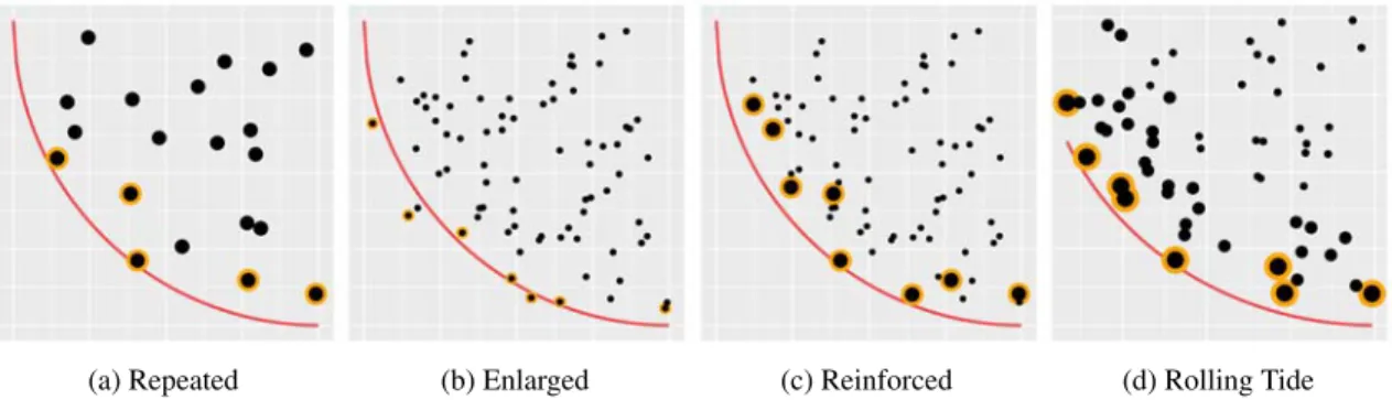
Figure 3.3 shows the resulting Pareto fronts of both tunings. ParEGO reaches a clearly better approximation of the Pareto front, it ﬁnds both more and better points than grid search. The most outstanding part of the fronts may be the cluster of points with an MMCE of 0.45. This MMCE equates to the ratio of the majority class in theeeg-eye-statedata set. Since the SVM falls back to predicting the majority class if parametrized poorly, many settings end up with that error.

The best found hyperparameter settings by ParEGO have MMCEs reaching down to 0.065, even better than the best settings from the single-objective tunings. Apparently, the increased bud-get does not just compensate for the additional parameter but also improves the optimization result. Moreover, since only 42% of the data are used to achieve this top performance, the training time

(27)

TUNING IN MIXED AND HIERARCHICAL PARAMETER SPACES 21 ● ● ● ● ● ●● ● ● ● ● ● ● ● ● ● ● ● ● ● ● ● ● ● ● _{● ●}● ● ● ● ● ● ● ● ● ● ● ● ● ● ●● ● ● ● ● ● ●● ● ● ● ● ● ● ● ● ● ● ● ● ● ● ● ● ●● ● ● ● ● ● ● ● _●_●_●●● ● ● ● ● ● ● ● ● ● ● ●● ● ● ● ● ● ● ● ● ● ● ● ●● ● ● ● ● ● ● ● ● ● ● ● ●● ● ●● ● ● ●_●● ● ● ● ● ● ● ● 1e−02 1e−01 1e+00 1e+01 1e+02 0.1 0.2 0.3 0.4 0.5 MMCE tr aining time 0.05 0.2 0.5 Subsample Rate

(a) Grid Search

● ● ● ● ● ● ● ● ● ● ● ● ● ● ● ● ● ● ● ● ● ● ● ● ● ● ● ● ● ● ● ● ● ● ● ● ● ● ● ● ● ● ● ● ● ● ● ● ● ● ● ● ● ● ● ● ● ● ● ● ● ● ● ● ●● ● ● ● ● ● ● ● ● ● ● ● ● ● ● ● ● _●●_● ● ● ● ● ● ● ● ● ● ● ● ● ● ● ● ● ● ● ● ● ● ● ● ● ● ● ● ● ● ● ● ● ● ● ● ● ● ● ● ● ● ● ● ● ● ● ● ● ● _● ● ● ● 1e−02 1e−01 1e+00 1e+01 1e+02 0.1 0.2 0.3 0.4 0.5 MMCE tr aining time 0.05 0.2 0.5 Subsample Rate (b) SMBO

Figure 3.3 Results from the multi-objective tunings for MMCE vs. training time, Pareto optimal points are marked in red.

is decreased to only 1.5 seconds. Further reductions of training data lead to further improvements in training time, but come with the cost of higher MMCEs.

3.3 Tuning in mixed and hierarchical parameter spaces

In the previous section the standard SMBO procedure was used, since all considered hyperparam-eters were continuous. However, many ML algorithms have discrete hyperparamhyperparam-eters. Further, if the learner itself is considered as an additional hyperparameter, also hierarchical parameters are present. Both discrete and hierarchical parameters can not be handled by the standard SMBO procedure. Horn and Bischl (2016) explain how it can be extended towards such mixed and hier-archical parameter spaces. This is achieved by adapting each individual SMBO step.

(1) Initial Design In most SMBO algorithms, LHS is used as initial design, which is deﬁned for continuous parameter spaces only. Horn and Bischl (2016) propose an alternative based on a thinning approach: First, a pure random design with sizec·ninit,c1, is sampled. Afterwards, pairwise distances between all design points are calculated and one of the two points with minimal distance is removed from the design repeatedly until the design is reduced to sizeninit. Thus it is ensured that no two points are too close to each other and the complete parameter space is covered. The approach leaves open the choice of an appropriate distance measure. For mixed and hierarchical parameter spaces, the Gower distance (Gower, 1971) may be used.

(2) The surrogate model Most SMBO approaches use Kriging or RBF models. Both model classes presume the parameter space to be continuous and, thus, they are not applicable here.

(28)

However, since any regression model can be picked as surrogate, they can be replaced by a more suitable one. Hutter et al. (2011) propose to use random forests, Horn and Bischl (2016) adopt this idea. RFs are a model class with many practical properties: They allow both continuous and discrete parameters and, given enough data, can model any functional relationship. Moreover, they often result in high-performance models even without hyperparameter tuning.

The handling of the hierarchical parameter space is a different matter. Even if theith parameter of a settingxxxis inactive, a valuexxxi is still available, although it does not have an inﬂuence on the objective function. Hence, the missing information has to be encoded in some way. Horn and Bischl (2016) propose to treat these values as missings. Although an RF can ﬁt a model on this missing values, a simple imputation technique should be applied to increase performance. Missing values of a continuous parameter X(i) _{are imputed with} _x(i)

right+2· x (i) le f t−x (i) right , i.e. a value outside its parameter space

x(_{le f t}i) ;x(_righti)

, for discrete features a new level is introduced. Since the trees of the RF perform splits based on single variables, it can split the data into active and inactive settings in a single node of each tree. Thereby it is ensured that the RF can still recognize and utilize the missing-information in the data.

(3b) Infill optimization In each SMBO iteration, the infill criterion has to be optimized. Since it is defined on the same parameter space as the target function, the optimizer has to operate on both mixed and hierarchical parameters. Since the evaluation of the infill criterion is cheap, it can be evaluated with a large number of different parameter settings. Therefore, even RS is a suitable alternative here. Horn and Bischl (2016) describe an enhanced version called focus search. It performs multiple RS iterations and, in between the iterations, shrinks the parameter space around currently found optima.

(3a, 4 – 6) Inﬁll criteria, Update, Termination, Return None of these three steps is affected by the parameter space and, thus, no adaption is needed.

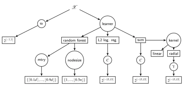
Horn and Bischl (2016) survey whether these adaptions result in a reasonable SMBO variant. In their experiments, the performance measures false-positive rate and false-negative rate are op-timized simultaneously on nine different binary classiﬁcation data sets, i.e. a ROC like curve is estimated.3 The multi-objective tuning is performed over three different model classes (RF, SVM and regularized logistic regression), where the choice of the model is a tuning hyperparameter itself. Moreover, weighting the positive class is allowed via weight-hyperparameter ω. Hereby each observation of the positive class is given the weight ω. Forω →∞, all observations will be classiﬁed in the positive class and therefore the false-positive rate will eventually be 1, while the false-negative rate will be 0, and vice versa forω →0. Hence, a trade-off between the two objectives can be achieved usingω. The resulting parameter space is shown in Figure 3.4. The adapted SMBO variant outperformed a baseline on nearly all considered data sets.