Family Background, School Quality, Ability and Student Achievement in Rural China –Identification Using Famine-Generated Instruments

Family Background, School Quality, Ability and Student Achievement in

Rural China

–Identification Using Famine-Generated Instruments

Qihui Chen

Department of Applied Economics, University of Minnesota, St. Paul MN55108

Selected Paper prepared for presentation at the Agricultural & Applied Economics Association 2009 AAEA & ACCI Joint Annual Meeting, Milwaukee, Wisconsin, July 26-29, 2009

Copyright 2009 by Qihui Chen. All rights reserved. Readers may make verbatim copies of this document for non-commercial purposes by any means, provided that this copyright notice appears on all such copies.

Family Background, School Quality, Ability and Student Achievement in

Rural China

–Identification Using Famine-Generated Instruments

Qihui Chen

Department of Applied Economics, University of Minnesota, St. Paul MN55108

This paper investigates the determinants of academic achievement in basic education (grade 1-9) for a sample of children (aged 9-12 in 2000) from rural China. A set of instrumental variable generated by the Great Famine in China, 1958-1961, is used to instrument an error-ridden measure of child innate ability, the cognitive ability score of each sampled child. Empirical results indicate strong effects of family background variables such as household income and parental education. Father’s education has significantly positive effect on academic achievements for both boys and girls, while mother’s education only matters for girls. Consistent with the common findings in the literature, most of school quality variables do not have significantly positive effects on child academic achievements.

Key words student achievement, school quality, ability, Famine in China 1958-1961

Education is widely seen as a key determinant of income growth in developing countries in the past decades (Psacharopoulos 1985, 1994). Evidence from rural China suggests that education has contributed to income growth in a number of ways, during China’s transition from a planned economy to a market economy since the early 1980s. For example, education raised farm income by enhancing managerial skill and labor productivity in agricultural production (Yang 1997a). More importantly, when restrictions on factor markets were loosen during the transition, rural households with better-educated members acted more quickly in allocating productive inputs to non-farm activities, capturing higher returns yielded by these activities (Yang 2004). For example, better-educated people tend to specialize in non-farm and better-paid jobs (Yang 1997b). In particular, people who had completed high school education were more likely to participate in non-farm employment than people with lower levels of education (Zhao 1999). Recent empirical evidence (de Brauw and Rozelle, 2008) also shows that the returns to post-primary education exceed the returns to primary education for off-farm workers in rural China.

Although less studied than other measures of educational outcomes (e.g., years of schooling), academic skills are shown to contribute to income growth. For example, math and English skills are found to have positive effects on household income in Ghana (Jollife 1998). In China, academic skills acquired at the basic education stage (grades 1-9) is of particular importance because admission into high schools is based only on students’ performance in their high school entrance exams. Only students that have acquired sound academic skills in their basic education can enter high schools and thus achieve higher earnings when they participate in labor markets where returns to high school education are high.

Child academic skills (measured as scores of academic achievement tests) are often determined by three sets of variables : family background variables such as household income

and parental education; school quality variables such as teachers’ experience and physical facilities; and child characteristics such as gender, age, and ability (see Haveman and Wolfe, 1995, and Glewwe 2002 for thorough reviews). The common findings in the literature are the positive and significant effects of family background variables (Behrman and Knowles 1999) and the statistically insignificant effects of school quality variables (Hanushek 2003). The strong associations between family background and child academic achievements have been well documented. For instance, the marginal benefits from investing in child education may be

positively correlated with household income, because richer parents can afford educational inputs of higher quality (Behrman and Knowles 1999). Better-educated parents might place higher value on child education and may be more able and more willing to help their children.

Family background would be expected to be important in determining child academic skills in rural China. For example, the funding structure of rural education suggests that household income matters. The fiscal reform in basic education in 1986 has shifted the financial responsibilities of funding basic education from central government to local governments and local communities.1 Local communities, in turn, raised funds by charging rural households high tuition and numerous fees (Tsang, 1996). Since rural households often do not have easy access to credit, household income is the major resource available to parents to pay for school education and other education inputs. Child characteristics might also matter. For example, in addition to genetic differences, the gender bias still prevalent in most rural areas suggests that gender will affect academic skills. Finally, school quality should also matter since formal education is the main channel through which rural children acquire academic skills. Unfortunately, despite the importance of academic skills to boost future income growth and the commitment of China’s

1

For example, rural primary school teachers are mostly non-government employees (known as min ban teachers), and they obtain their salaries from the local communities, not from the state or provincial government.

government to continue to alleviate rural poverty, few studies have focused on analyzing which factors are among the most important determinants of academic skills in rural China.4 As a result, policy makers have little empirical evidence that they can base on to decide what to invest in to raise academic skills of rural people in China.

In addition to the lack of research inside China, empirical analysis might suffer from econometric problems among the existing studies (Glewwe and Kremer, 2006). For example, the omission of child innate ability could bias the estimated effects of family background variables. Because children’s innate ability and parental ability are genetically interlinked, children’s innate ability is correlated with parental education and household income, which are determined by parental ability. Also, the failure to control for unobserved school quality variable has been found to be another source of omitted variable bias (e.g., Glewwe et al. 2004). Unobserved school quality may bias estimates of the impacts of school quality variables. Moreover, it may also lead to biases in the estimated impacts of family background variables. The is because family

background and school quality are likely to be correlated due to parents’ behavioral responses to school quality known to them but unobserved by researchers. Hence, in order to obtain consistent estimates, it is important to deal with these estimation problems.

This paper has two goals. The first is to analyze the determinants of academic skills acquired in basic education in rural China. The second is to investigate the potential biases that arise from the failures to control for unobserved child ability and unobserved school quality. Clearly, any empirical analysis will only be consistent and reliable for policy concerns after potential biases are carefully accounted for. Therefore, the sizes and the directions of biases caused by these two sources of omitted variables will be assessed in this paper.

4

This paper makes two contributions in achieving these two goals, one empirical and one methodological. Empirically, this paper is one of the few studies that look at the determinants of child academic skills acquired in basic education in rural China. Methodologically, the main novelty of this paper is the development of an instrumental variable (IV) procedure to control for child ability. A “natural experiment” generated by the 1958-1961 famine in China, is used to construct a set of instrumental variables for an error-ridden measurement of innate ability (a cognitive ability test score).

We begin the rest of the paper by developing both the conceptual framework and the estimation framework of demand for academic skills. We also discuss potential identification issues and develop possible identification strategies. Some facts in the Great Famine in China, 1958-1961, and the IV generated by the Famine are then discussed. Next, we detail the data used in this study and estimation results in the empirical analysis. Summary and concludes are provided at the end of this paper.

Conceptual Framework

The demand for academic skills

This section sketches a simple conceptual model for thinking about the relationships between child academic skills and the set of determinants. This sub-section derives the demand function for child academic skills, which forms the basis of our empirical analysis. The next sub-section discusses the effects of family background and school quality on child academic skills. In particular, the analytics provides some insights on the directions of these effects, which have been overlooked in previous studies.

(1) U = ( ,U C H),

where C is the composite household consumption good and H stands for child academic skills, as measured by academic achievement test scores. The household faces two constraints in the maximization process: the budget constraint and the technology constraint.

The household budget constraint is defined as:

(2) _{j j}

j

C +

∑

where Ij is the j-th element of the educational input vector, I, pj is the corresponding j-th element

in the price vector, p; m is the total amount of monetary resources available to the household. The vector I includes years of schooling and other educational inputs, such as textbooks, extra reading materials and tutoring services. Correspondingly, p may include tuition, school fees and the cost of tutoring.

The technology constraint is expressed as a production function of child academic skills: (3) H = H_P( ; , , )I k f q ,

where the subscript P denotes HPas a production relation. The vector k is a set of child (kid)

characteristics, including gender, age and innate ability (denoted A). The vector f is a set of household characteristics, say, parental education. The vector q represents school quality including teacher experience, quantity/quality of the physical facilities and other aspects. HP (·) is

assumed to have usual properties of a production function, e.g. concavity and differentiability, to ensure that maxima are achievable in the household equilibrium. Note that variables in vector I

are all endogenous, while variables in k, f, q are all exogenously given.5 By including these

5

School quality q could be endogenous if multiple schools of different qualities were available for households to choose from (Glewwe and Jacoby 1994). If this were the case, schools of higher quality might attract children with higher ability. Then school quality would then become endogenous when ability is not controlled for and thus left in the error term. However, in China, a child is restricted to enroll in nearest school that is located in the districts where his/her family reside in. Because of this, q can be reasonably treated as exogenous in our setting of rural China.

exogenous variables in the production function, we allow for heterogeneity in the production technique used to produce academic skill across families and schools.

Solving the optimization problem (1), subject to constraints (2) and (3), yields the following demand functions:

(4) C = ( , ; , , )C p m k f q , (5) I_j = ( , ; , , )I_j p m k f q .

Equation (4) is the demand function for household consumption, and equation (5) is the demand function for educational input. Substituting (4) and (5) into equation (1), we obtain the demand function for child academic skills:

(6a) H = H_P( ( , ; , , )); , , )I p m k f q k f q .

Since each element of the vector I is also a function of the same set of exogenous variables, (p,m;

k, f), equation (6a) can also be expressed as the following equation: (6b) H = H_D( , ; , , )p m k f q

Because variables in (6b) are all exogenous, equation (6) is a reduced form demand equation (as opposed to the structural relationship in equation (3)). The subscript D denotes HD as a demand

function. From the above derivations, one can see that the reduced form relationship characterized in equation (6b) takes into account the behavioral adjustments to I in response to exogenous shocks in any exogenous variable in (p, m, k, f, q), while holding others constant. Because of these, equation (6b) is probably the most relevant for policy makers (Blau, 1999), and thus is of the main interest in this paper and the basis of empirical analysis in the later sections.

Linearizing equation (6b), we have the following estimating equation: (7) H = xβ +qη+ αA+ ε ,

where x = (p, m; k, f) is the matrix of all (unobservable) exogenous variables, and ε is the error term. Child ability A and school quality q are listed separately because they are the sources of potential biases in estimation that will be discussed in more detail in section 3 below. Equation (7) is the equation that will be estimated in the empirical analysis.

Effects of family background variables and school quality variables

In this section, we examine the effects of family background variables and school quality variables in more details. In equation (7), each element in the parameter vector β and η captures the total effect of an exogenous change in the corresponding element in x and q, holding other variables constant. Since the total effect incorporates indirect behavioral adjustments, the structural relationship in equation (3) will also assist in analyzing the effects of x and q on H.

The effects of family background variables, f, are expected to be positive. Consider the effect of the l-th variable in f, say, father’s education, fl. Differentiating both sides of equation (6a)

with respect to fl, we have:

( ( , ; , , )); , , ) j D P P P j l l j l l I H H H H m f f I f f ∂ ∂ ₌ ∂ ₌ ∂ ₊∂ ∂ ∂ I p k f q k f q

∑

The left hand side, i.e., D l H f ∂

∂ , measures the total effect of father’s education on child academic skills. The total effect D

l H f ∂

∂ is composed of two distinct effects: the direct effect of fl on HD that

is captured by the term P l H f ∂

∂ and the indirect effect of fl on HD, captured by the term

j P j j l I H I f ∂ ∂ ∂ ∂

∑

which works trough parental behavioral adjustments I, j l I

f ∂

∂ . Since each exogenous variable is expected to have a positive effect on the acquired academic skills in the production function

(equation (3)), both P l H f ∂ ∂ and P j H I ∂

∂ are positive. Additionally, 0 j l I f ∂ > ∂ since more-educated parents are expected to be more able and more willing to invest in their children.

Then P j I j l I H I f ∂ ∂ ∂ ∂

∑

they are both positive.

The effects of school quality variables can be derived in the same fashion. Differentiating both sides of equation (6a) with respect to the k-th school quality variable, qk (say teacher

experience), we have D P j P j k j k k I H H H q I q q ∂ ∂ ₌ ∂ ₊∂

∂

∑

q ∂

∂ ,

includes both the direct effect P k H

q ∂

∂ and the indirect effect

j P j j k I H I q ∂ ∂ ∂ ∂

∑

However, the direction of the total effect is not unambiguous. Since both P k H q ∂ ∂ and P j H I ∂

∂ are positive, the sign of kD H

q ∂

∂ is determined by the sign of j k I q ∂

∂ , which captures the

adjustments in educational inputs by parents in response to variation in school quality. If j k I q ∂ ∂ were positive, D k H q ∂

∂ would be unambiguously positive. However, j k I q ∂

∂ could also be negative. This would occur if parents respond negatively to school quality qk, that is, if parental inputs are

substitutes to school quality. For example, parents might reduce their educational inputs, e.g.,

stop hiring tutors if they know their children are enrolled in a good school. When j k I q ∂ ∂ is negative,

6 _{The latter holds other things constant while the former does not. As has been correctly pointed out by Glewwe and Kremer}

(2006), different effects found in different studies do not necessarily imply the existence of biases; they could merely represent effects of variables in different underlying relationships.

the sign of D k H

q ∂

∂ is determined by the relative magnitude of the indirect effect

j P I j k I H I q ∂ ∂ ∂ ∂

∑

the direct effect P k H

q ∂

∂ . If the educational inputs have large direct effects on academic achievement, i.e., P j H I ∂ ∂ is large in magnitude, kD H q ∂

∂ could even be negative. The possibility that

0 D k H q ∂ _<

∂ suggests that negative impacts of school quality variables found in some previous studies7 are not necessarily counterintuitive and do not necessarily imply the existence of biases; it could simply be reflecting that parent inputs and school quality are substitutes.

Identification Issues

Although the estimated effects of exogenous variables in the reduced form have important policy implications, they are reliable only when possible biases in econometric analysis are ruled out. Also, causality between these effects and child academic achievements can be established only if possible confounding factors are appropriately controlled for. The two factors that are most likely to cause biases are the unobserved school quality q andthe child’s innate ability A, which have been highlighted explicitly in equation (7). If child ability A is omitted and if A is correlated with any variable in x, the estimates of the parameters associated with those variables, and probably all variables in equation (7), will be inconsistent, by standard econometric theory. The same situation occurs when one or more elements in q are omitted. The following subsections discuss these possibilities.

Unobserved school quality

7

The possibility of omitted school quality variables is suggested by the finding that the impacts of school characteristics on student achievement are often statistically insignificant (Glewwe and Kremer 2006).8 By comparing prospective estimates and retrospective estimates using data in Kenya, Glewwe et al (2004) find evidence of omitted school quality variables, even when controlling for other observable school quality variables.

Obviously, the omission of some school quality variables can lead to biases in the estimated effects of the school quality variables that are included in the regression. The quality of school is reflected in many dimensions. Moreover, variables that measure different dimensions of school quality could be correlated to each other. For example, a school with good reputation might attract both better teachers and more social investments in physical facilities, and thus reputation, teacher quality and physical facilities are correlated. However, some dimensions of school quality are more difficult to measure than others. Such school quality variable as reputation is difficult to measure and thus is likely to be omitted. As a result, the estimated effects of school quality variables could be biased. The directions of possible biases would depend on whether the omitted school quality variables are substitutes or compliments to the school quality variables that remain in the regression.

Similarly, the omission of some elements in q could lead to biased estimates of the effects of x. The directions of such biases depend on whether family background variables, such as parental education, are substitutes or compliments to school quality.

Unobserved Ability

8 _{Some studies have tried to include many school quality variables in an attempt to avoid the omitted variable problem. For}

example, the Jamaican study by Glewwe et al. (1995) used more than 40 school characteristics variables. However, their findings show that most variables are still statistically insignificant.

Ability can never be perfectly observed. The omission of child innate ability could lead to upward biases on the estimated impacts of family background characteristics (Behrman and Rosenzweig, 1999). The omitted variable bias arises because child innate ability A and family background f are often correlated. For example, A is positively correlated with f through the genetic link between child ability and parental ability and the effect of parental ability on f. Furthermore, A and f could also be correlated through parents’ behavioral response to child ability. This correlation and thus the directions of biases in estimated effects of f caused by omitted ability are theoretically ambiguous.

Intelligence Test Score as Imperfect Proxy for Unobserved Ability

Another problem caused by unobserved ability comes from the attempts to control for child ability in practice. To avoid omitted ability biases, many studies have used some measure of the innate ability, most often the score of an “Intelligence” test (ITS), as a proxy variable for innate ability. For example, Kingdon (1996) used Raven’s Coloured Progressive Matrices test score as a proxy of innate ability and replaced A directly with the Raven’s score in the regression. However, none of the measurements available now can perfectly measure innate ability. They can at most serve as an “imperfect proxy” for ability. The use of imperfect proxy will probably lead to biased estimates.

The biases caused by directly applying the proxy variable solution, i.e., replacing ability A directly by the imperfect proxy, ITS, can be seen below. In theory, one can always write a linear projection of ITS on the innate ability A as L(ITS|A ) = γAA. Then, ITS can be redefined by adding

a residual term e that is uncorrelated with A: (8) ITS ≡ γAA + ,e

However, in addition to A, the ITS score could also reflect the influence of environmental factors (American Psychological Association 1995) and the test-taking skill that are not correlated with A. Most relevant for our case, one set of environmental factors includes a subset of school quality variables in q. Since China’s policy regarding school enrollment rules out the correlation between school quality and child ability, q will remain in e. Then equation (8) becomes:

(9) ITS ≡ γ_AA + qδ+ ,u

where u includes other environmental factors that are either uncorrelated with A or that are random. Simple algebra yields:

(10) A A A ITS u A γ γ γ = −q δ − .

Inserting (10) into (7), we have:

(11) ( ) A A A H A ITS u α ε α α α _ε γ γ γ = + + + = + − + − + xβ qη xβ q η δ

When A is replaced by ITS, equation (11) is estimated instead of equation (7). There are at least two problems with estimating equation (11). First, if some components in δ are nonzero the estimates of coefficients on q are biased. The estimates are off by the magnitude of

A α γ −δ .

Furthermore, the bias cannot be corrected because δ and γA are not estimable (since A is

unobserved). Second, when equation (11) is estimated, ITS will be correlated with the error term

A u

α _ε

γ

− + through its correlation with u. Consequently bias arises. In contrast to the first

problem, the second problem, which is similar to the usual measurement error problem, can be solved using an instrumental variable approach to eliminate the correlation between ITS and u. Furthermore, in practice, there are always possibilities that some components in q are omitted.

Estimates of the effects of q could still be biased even when the second problem is eliminated. Hence, in order to eliminate possible biases due to unobserved school quality and unobserved child ability, one needs to control for them simultaneously. The strategy used in this paper, the IV-fixed effect approach will be discussed next.

Identification Strategies

If information on multiple students enrolled in the same schools is available, a natural method to control for unobserved school quality is simply to use school fixed effects. Take equation (7) for example, for the i-th student in the m-th school, the achievement demand function can be rewritten as, (7’) im im im m im im im m im H A A s α ε α ε = + + + = + + + x β q η x β

The vector of school quality, qm, are constant across all students in school m. The entire set of qm,

together with its coefficient vector η, can be pooled into a school-specific constant, sm (=qmη).

Then the usual fixed effects estimation procedure applies. The fixed effect estimator is attractive because it allows x to be correlated with unobserved q variables since the latter are included in the regression through sm. Note that the term sm captures the effects of all school level

characteristics that do not vary within school m, both observed and unobserved.

Even when school fixed effects are controlled for, one still needs to control for the unobserved child ability Aim in equation (7’) above. Since this paper also uses an ability measure9

to control for unobserved innate ability, the identification issues caused by imperfect proxy for

9

In this paper, child ability is measured by the score of a cognitive ability test that was administered to each sample child in 2000 when almost all the sample children were enrolled in primary schools.

child ability must be addressed here. The IV solution applied in this paper is the approach proposed by Griliches and Mason (1972) and also applied in Blackburn and Neumark (1992). The idea is to treat ITS as an indicator, instead of a proxy variable, of the true innate ability, and then apply standard IV procedures to this indicator.10 When an error-ridden measure of child ability (IQ) is available, equation (11) highlights the needs to apply fixed effects and IV estimation techniques simultaneously. The term _m( )

A α γ −

q η δ in (11) is simply absorbed into the term sm, and then equation (11) becomes:

(11’) = ( ) = im im m im im im A A A im m im im im A A H ITS u s ITS u α α α _ε γ γ γ α α _ε γ γ + − + − + + + − + x β q η δ x β

Controlling for school fixed effects, consistent estimates of the effects of family background variables can be obtained if plausible instrument variables are available. The next section describes the set of suitable IV used in this paper.

Famine in China, 1958-1961 and the Famine-generated IVs

Good IVs are difficult to find. But history helps. A natural experiment generated by the Great Famine in China, 1958-1961, provides candidates for the IV needed. The famine resulted from the agricultural crisis in 1958 and the following political decisions regarding food allocation.11 At the national level, grain production plunged by 15 percent in 1959 from its peak of 200 million tons in 1958. It declined by another 15 percent in 1960 and stayed flat in 1961 (State Statistical

10

One possible approach can be found in the Ghana study by Glewwe and Jacoby (1994). The authors extracted an innate ability factor as a household fixed effect, using parental ability measures. In other words, the ITS variable, i.e. the Raven score of the child, is instrumented by using father and mother’s Raven’s scores and other exogenous variables. Note that this approach is valid only if measurement errors in parental ability and child ability are uncorrelated. Also, because parental ability measures are not available in the data set used in this paper, other possibly suitable IVs are needed.

11

Detailed analysis of the causes of this famine can be found in Lin (1990), Lin and Yang (1998), Lin and Yang (2000), among others.

Bureau, 1991). In addition to the food shortage caused by the declined agricultural output, food allocation decisions that set high priority to urban food consumption, established during that period exacerbated the shock of original output decline in the rural area (Lin and Yang, 2000). To guarantee the success of the Great Leap Forward in 1958, Chairman Mao’s ‘One Chessboard’ speech in the spring of 1959 reaffirmed the urban bias in food allocation and gave a high priority to city grain supplies over rural localities.

The famine in 1958-1961 is now recognized as the worst in human history. It has been estimated that the famine caused excess deaths of some 30 million of people and lost births of more than 30 million, mostly in rural areas (Ashton et al. 1984). Gansu province, the study area in this paper, was seriously affected by the famine and the urban-biased policies that followed. The administration extracted 361 thousand tons of grain from Gansu to support the urban food supply between 1959 and 1960 despite the food shortage in the province (Walker 1984). At the same time, the rigorously implemented residence registration (Hukou) system prevented rural people from migrating to urban areas. As a consequence, death rates increased dramatically in Gansu: 11.1 ‰ in 1957, 21.1‰ in 1958, 17.4 ‰ in 1959, 41.3 ‰ in 1960, and 11.5 ‰ in 1961. The death rate in Gansu in 1958 was the third highest among all 28 provinces for which data were available.

It is clear that the famine cohort, people who were born during or slightly before the famine period (i.e. people who spent their early childhoods during the famine) and survived could be a very different cohort. In particular, people in the famine cohort might have higher ability endowment than those who failed to survive and those who were born after or long before the famine because the famine “selected” out people with higher ability.12

12

Note that there is no contradiction between this argument and that in Chen et al (2007). Famine could not only select out people with high endowment, but also affect their lives badly ever since. The idea here is that, their high endowment could have been

In addition to the selection effect, the famine can also have a somewhat offset effect on parents’ ability through poor prenatal nutrition intake. Recent studies on the long-term impacts of the famine (Chen et al. 2007) indicates that people born during the famine period have significantly lower heights than they would otherwise have had, which implies low nutrition intakes during the famine. Early prenatal nutrition has been found to be essential in human brain development. For example, Villar et al. (1984) found that infants whose head growth slowed due to poor prenatal nutrition before 26 weeks of gestation (as measured by ultrasound) grew slower than otherwise, and scored lower in mental performance in preschool years. Similarly, one would expect the famine-born cohort to have lower ability than they would otherwise. This nutrition effect could offset the effect the famine selection on high ability.

If some of the parents of the sample children belong to the famine cohort, then famine can serve as an IV for three reasons. First, there is a large literature showing that parents’ innate ability is closely correlated with their children’s innate ability. Second, since the famine affects parents’ ability, either through the selection effect or through the poor prenatal nutrition effect, the famine is likely to be correlated with children’s ability. Third, assuming equation (7) is fully specified, controlling ability A, famine will not have explanatory power on child academic achievement. In other worlds, the famine can affect children’s academic skills only through its effects on children’s innate ability in a fully specified model.

Data

The data used in this paper come from the Gansu Survey of Children and Families (GSCF). This longitudinal survey follows 2000 sample children over years (2000, 2004 and 2007) in Gansu, a poor province located in northwestern China. During the survey, a stratified sampling strategy

was first used to select 20 counties from all non-urban, non-Tibetan counties in the province. Within each of the 20 counties, 5 villages were selected. Within each village, 20 children in the correct age range (9-12 in 2000) were randomly drawn. Separate questionnaires were administered to the sample children, their parents, local village leaders as well as to teachers and principals of the schools the sample children enrolled in at the time of the survey.

This paper uses only the 2004 cross-section of the GSCF panel. In this sample, all children were enrolled in grades 1-9. This sub-sample was chosen for two reasons. First, basic education is an important issue in China. Nine years of basic education has been made compulsory in China since 1986, and the universal completion of basic education is one of the main goals of China’s educational policy (Tsang 1996). Second, using this sub-sample rules out selectivity issues caused by schooling choice in selecting high schools. Since high school admissions decisions in China are based on students’ performances in high school entrance examinations, school quality will be correlated with student ability and student achievement acquired in basic education, for high school students. Thus, including high school students in our analysis will bring about both selectivity and simultaneity issues in estimation.

The dependent variables are child academic skills measured by math test scores. In 2004, a math test was administrated to all sample children. All children used the same test instrument, which ensures that academic skills are measured by math score at the same level of difficulty. Note that those sample children that were interviewed in 2000 but dropped out since then also took the academic achievement tests in 2004. The inclusion of these children eliminates sample selection biases caused by dropping out of school.

The most important family background variable is the household income per capita. In household surveys, household income is often subject to measurement error caused by

under-reporting (Deaton 1997). Household expenditure is often a better measurement of household income. However, since household expenditure data is often recall data, it is susceptible to measurement error unless household members keep a detailed record of daily consumption. To deal with measurement error in expenditure data, household wealth per capita in 2000 is used as an instrument variable. The household wealth is calculated as the total value of house assets plus the value of the house. During the survey, the enumerators conducted the interviews in the household residence and thus were able to record all the assets households had. Since the household wealth came from record data, it does not suffer from measure error problems. Also, as a long term (probably 5-10 years) decision, educational investment should depend on long term household resources instead of current yearly household resources. Using wealth in 2000 as instrument for household expenditure is similar to exacting a long term wealth component from the current household resource measure. In all regressions below, the logarithm of household expenditure per capita is instrumented by the logarithm of household wealth per capita in 2000.

Other family background variables include parental education, number of younger siblings and number of older siblings, and dummy variables indicating whether the parent in living in the household. A parent is defined as not living in the household when he or she has been living outside the household for at least three months during the survey year. This variable reflects labor market conditions and future return to schooling for the child in terms of information on urban labor market and migration networks. Similarly, landholding per capita is included to capture future occupational choice of the child.

Child characteristics include gender, child age measured in month, and its square. A cognitive ability test was administrated to each sample child in 2000 when they aged 9 to 12, which serves as the (error-ridden) measure for child innate ability.

School quality variables used here include the most commonly used ones in previous studies, such as student-teacher ratio and teacher experience (the share of teachers with more than 5 years’ teaching experience). A set of physical facility variables that have been used in China studies by Brown and Park (2002), and Zhao and Glewwe (forthcoming) is also included. This set of physical facility includes the fraction of dangerous classrooms, the fraction of rainproof classrooms, and the fraction of classrooms that have good condition of light. Finally, a set of dummy variables indicating the existence of libraries, computers, science labs and whether desks are available to all students in the school is included. Table 1 summarizes definitions and summary statistics of the key variables used in empirical analyses below.

Empirical Results

Evidence of cognitive ability score being imperfect proxy for true ability

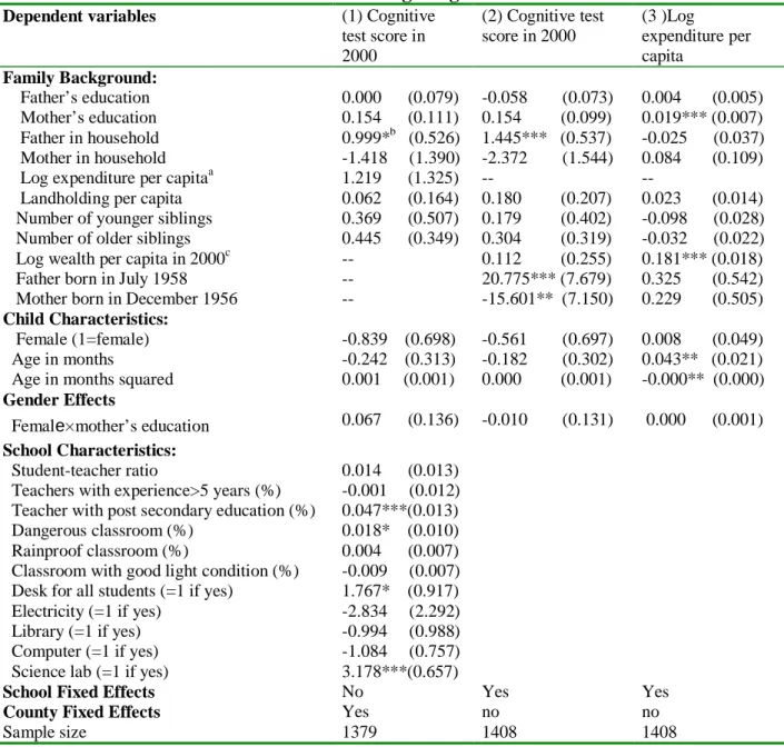
Before reporting the results in the academic skills demand function estimations, it may be helpful to provide evidence that supports the rationale of the fixed effect-IV estimator discussed above. The rationale comes from equation (9). Equation (9) points out that the ability measure, ITS, might include both effects of some school quality variables (q) and random measurement error (u) that are not components of child ability, A.

To examine this possibility, a version of equation (9) is estimated, using all exogenous variables mentioned above:

(9’) ITS = qδ+xθ+γ_AA + ,u

where child innate ability A is not observable in equation (9’), and thus A enters the composite error termγ_AA + u. Since A is not correlated with q given China’s policy regarding basic education, leaving it in the composite error term will not cause biases in the estimated

coefficients on q13. Hence, any significant effects of school quality will lend support to the hypothesis that either δ ≠ 0 or some school quality variables are omitted. The estimation results (column (1) in table 2) show that two school quality variables, i.e., teacher experiences and the existence of science labs have positive effects on ITS, at the five percent level. For example, students enrolled in a school with science labs are estimated to score more than three points higher than students enrolled in a school without science lab. This finding suggests that either δ≠

0 or some school quality variables are omitted. 14 In either case, the school fixed effects estimator is appropriate to control for school quality.

Demand for academic skills

This section reports estimates of equation (11’), for math score. Ideally, when estimating the reduced form demand functions, one should include all prices variables, e.g. prices for consumption goods and prices for educational inputs. Since the consumption good has been treated as numeraire in the conceptual model, we simply add county dummies in regressions to control for local prices. County dummies also control for labor markets conditions and possibly future return to education. All endogenous variables, such as years of schooling and parental time spent helping with child homework, are excluded, for the reduced form regressions. Furthermore, several interactions are explored. For example, interaction between gender and parental education, interaction between parental residential status and parental education are included. However, none of these interactions, except the interaction between gender and mother’s education, is

13

Note that omitted school characteristics variables can lead to biases in estimated coefficients on q here. But this also lends support to our fixed effect strategy to control for unobserved school quality.

14

Another interpretation is that this variable captures the effect of unobserved school quality. Note that significant effect of science lab is also found in Zhao and Glewwe (forthcoming). Using the same data as ours, they find that schools with science labs keep students in schools longer before they dropped out of schools. However, it is hard to establish causality between science labs and dropout decisions. A more plausible explanation is that science labs pick up, at least partly, the effects of some unobserved school quality: it is the unobserved school quality (e.g., school reputation) that keeps students in school longer. Along the same line, our finding here suggests that some unobserved school quality variables.

found to be significant predictors of student achievement at five percent level. Therefore, only the interaction between gender and mother’s education is included below to capture gender effects.

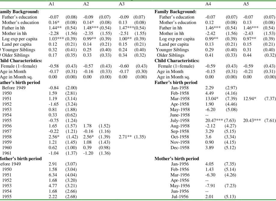
These significant predictive powers of endogenous variables in the first-stage regressions (column (2) and (3) in table 2) indicate that our IVs might not suffer from the weak IV problem. The instrument for household income (as measured by the logarithm of annual expenditure per capita) is the logarithm of household wealth per capita in 2000. As can be seen in column (3) in table 2, the logarithm of household wealth per capita in 2000 has strong predictive power of logarithm of annual expenditure per capita (p = 0.0000). The (famine-generate) IVs for ITS, the cognitive ability score are dummy variables indicating that the father was born in July of 1958 and that the mother was born in December of 1956.15 They are jointly significant at p = 0.0000 level in the first-stage regression (column (2) in table 2).

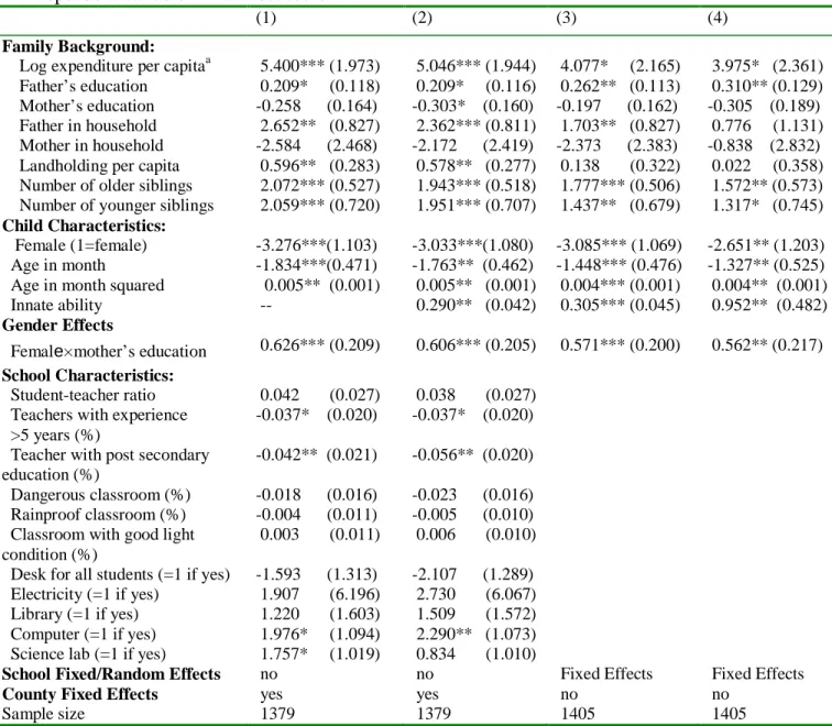
Effects of school quality variables

Columns (1) and (2) in table 3 report the effects of school quality on students’ math achievements. Column (1) leaves ability A in the error term, while column (2) adds ITS as a proxy variable for innate ability A. The estimated effects of school quality could be biased, however, due to the two possible sources of bias discussed above: omitted school quality variables and the school quality measured in ITS. Nevertheless, the bias in the estimated effects of school quality in column (1)16 is expected to be smaller than that in column (2). This is because estimated effects of school quality in column (1) will not suffer from the second source of bias, since A is left in the error term and A is not correlated with q in our sample.

15

The construction of this set of famine-generated IV can be found in Appendix II.

16

Consistent to the findings in previous studies, most of the school quality variables do not have positively significant effects on students’ math skills (column (1) in table 3). The two teacher quality variables, the proportion of teachers with more that 5 years of teaching experience and the proportion of teachers with post-secondary degrees, have significantly negative effects on student math achievement. For example, increasing one percent of teachers with more than five years of teaching experiences is associated with a decrease in math score by -0.04 points. Note that as has been discussed above, the negative effects are not necessarily implausible; they could result from parents’ investment behavior in responses to school quality.

The only two variables that have significant effects in column (1) are the existence of computers and that of science labs. Note that Zhao and Glewwe (forthcoming) find schools with science labs keep students longer in schools using the same data set used in this paper. However, it is difficult to establish causality between science lab and dropout decisions and better math achievements. A more plausible explanation is that science labs capture the effects of some unobserved school quality; it is the unobserved school quality (e.g. school reputation) that keeps students in school longer and contributes to students’ math skills.

Adding the ability measure ITS in the model (column (2) in table 3) does not change the signs of the estimated effects of school quality variables, but it does change the magnitudes of some estimated effects. For example, the effect of teachers’ experience becomes more negative (-0.056). This is expected because it has been shown in section 7.1 (column (1) in table 2) that teachers’ experience has a significant positive effect on ITS. Also, the significant effects of science labs disappear when ITS is added. This is also expected given the strong positive effect of science labs on ITS score (column (1) in table 2). Given that ITS serves as an imperfect proxy for

child ability, A, we believe the estimated effects of school quality in column are believed to be more plausible.

Although some significant effects of school quality that consistent to previous findings are found, the effects of school quality could still suffer from bias due to omitted school quality variable17, and thus one needs to interpret these effects of school quality with caution.

Effects of family background variables

We have pointed out above that unobserved school quality may cause bias in the effects of family background variables. Thus, we only discuss the estimated effects of family background in the fixed effects-IV estimations (column (4) in table 3). As expected, most family background variables have significant effects for math score in 2004, controlling for both school quality and child ability (column (4) in table 3). First, the effect of household income is positively significant. Since household income is measured in the logarithm scale, one percent increase in household income is estimated to be associated with 0.04 points increase in math score; or equivalently, doubling income is associated with 4 points (or 0.3 standard deviation) increase in math score. Note that for households in our sample, the mean annual household expenditure per capita was only 1276 yuan in 2004, which was equal to 155 U.S. dollars in 2004. This means that doubling household income for an average household is not very demanding, and transferring cash to poor household could have big effects on child academic achievement.

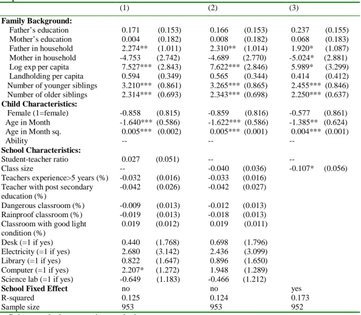
17

A simple data experiment is used to explore this possibility, and this simple experiment offers evidence of omitted school quality variable. The data set includes one variable, the class size at the class level, as opposed to the school level. This variable enable us to compare the estimated effects of class size before and after school fixed effects are controlled for since class size has extra variation after school fixed effects are controlled for. The results of this data experiment are reported in table A1 in

Appendix. Note in table 3, we use student-teacher ratio for the full sample, because the class size variable is available for only 952 observations. To ensure that results are comparable when we replace student-teacher ratio by class size, column (1) in table A1 repeats the exercise of column (1) in table 3, using only observations with variable class size available, while column (2) in table A1 replaces student-teacher ratio by class size. It can be seen that this simple substation does not change much of the result, except that the class size variable has a negative impact on student achievement. Column (3) in table A1 controls for school fixed effects. After controlling for school fixed effects, the impact of class size becomes negatively significant at 10% level, which is more close to common sense and provides evidence of omitted school quality variables.

Second, parental education has significant impacts on child math achievement, but the effects of father’s education and mother’s education differ. Other things being equal, an additional year of father’s education is associated with about a 0.3 point increase in math achievement, for both boys and girls (since interaction between gender and father’s education is not significant and thus is excluded). In contrast, mother’s education matters only for girls, and the effect of mother’s education is almost doubled in size as that of father’s education. The finding that mother’s education plays different roles in boys and girls’ math achievements suggests potential gender bias in education decision makings. The finding that girls scored significantly (three points) lower than boys and the fact that more than 500 mothers’ in the sample have never been in schools imply that females have been discriminated against for more than one generation in terms of education in rural Gansu. Thus, one possible explanation for the differential effects of mother’s education for boys and girls is that more-educated mother might provide a role model for girls, who provide higher motivation for their daughters who would be discriminated against otherwise. This lends supports for designing policy to raise female education in order to reduce gender inequality in the future.

The number of siblings, either younger or older, has positive effect on math achievement. Significant sibling effects indicate that children may benefit from helping each other at home. In other words, learning in family is a public good within the household.

Potential biases

Although the actual size of biases cannot be calculated here because the columns in table 3 use different estimators. However, we can get some information about these biases by comparing estimated effects across columns in table 3. The total biases caused by both

unobserved school quality and child ability can be assessed by comparing coefficients in column (1) and column (4). Income effects are overestimated (column (1)) to be about 1.5 points (or 75 percent) higher than the consistent estimates (3.97 points) in column (4), when one does control for either unobserved school quality or child ability. Also, the effect of father’s education is underestimated in column (1). The biases caused by unobserved school quality (by comparing column (3) and (2) in table 3) have the similar effects as the total biases discussed above.

Comparing columns (3) and (4) in table 3 provides some information on the biases caused by random measurement error (u in equation (9), not the part that caused by school quality) in the ability measure. The large increase in the coefficient on the child ability measure (from 0.3 to 1) indicates the existence of attenuation bias caused by measurement errors. The biggest bias in other estimates is the estimated effect of fathers living in the household. Column (3) suggests that father living in the household can increase math score by 1.7 points, controlling for income and father’s education. But this effect is no longer significant when the famine-generated IVs are used. These imply that having a migrating father is not necessarily harmful for child education; this is probably because fathers that participate in migration in rural China are mostly temporary migrants and they do spend a certain amount at home each year. In short, the bias caused by u is probably not a serious problem when school fixed effects are controlled for. This suggests that the biases caused by failing to control for unobserved school quality may be more serious than measurement error in the ability measure.

Summary and Conclusions

This paper investigates the determinants of academic skills acquired in basic education for a sample of rural children (in grades 1-9) from Gansu, China. Consistent with the common findings

in the literature (without controlling for school fixed effects), most school quality variables do not have significantly positive effects on child academic achievements. Teacher quality variables, i.e., teaching experience and degree held, have significantly negative effects on child academic achievements. Although they seemed counterintuitive, they are plausible if parents behave negatively in response to school quality. The existences of computers and science labs, in contrast, are found to have significantly positive effects on child academic achievements.

However, given the possibility of omitted school quality variables, we interpret this finding with caution. It could be that the existence of science labs captures some unobserved school quality variables, e.g., school reputation, and it is these unobserved school quality variables that contribute to student achievements. Without further information, we cannot conclude these significant effects are indeed the causes of student achievements, and thus we defer policy implications to future research.

The causality between family background and student achievement can be established with more confidence using our school fixed effect-IV estimator using the famine-generated IVs. Significant income effects are found in reduced form estimations, which imply that governmental transfer programs might have big effects in raising child academic achievement. For example, A cash transfer of 150 U.S. dollars can increase the child’s math achievement by 4 points ( or 0.3 standard deviations) for an average household. Father’s education has significant impacts on both boys’ and girls’ academic skills. However, the magnitudes of these effects are small, which is consistent with the common finding in previous studies (Behrman and Knowls 1999).

Interestingly, mother’s education is significant for girls only, suggesting that the possible existence of gender bias in investing in child education in rural China. Given the evidence that

girls perform significantly lower than boys, raising mother’s education may have an important impact on closing gender inequality in rural China.

Biases caused by unobserved school quality and unobserved child ability are also assessed. Although they can both cause biases in the estimates of family background effects, the biases caused by unobserved school quality are more serious than that caused by unobserved child ability. This finding points out the need to develop methods for appropriately controlling for school quality in future research in child educational outcomes.

References

Ashton, B., K. Hill, A. Piazza, and R. Zeitz. (1984). “Famine in China, 1958-61.” Pop. Develop. Rev. 10(4): 613-45

Behrman, J. R., M.R. Rosenzweig, and P. Taubman. (1994). “Endowments and the Allocation of Schooling in the Family and in the Marriage Markets: The Twins Experiment.” J. Polit. Econ. 102(6):1134-74

Behrman, J. R., and M. R. Rosenzweig. (1999). “‘Ability’ biases in schooling returns and twins: a test and new estimates.” Econ. Educ. Rev. 18(2):159-67

Behrman, J. R., and M. R. Rosenzweig. (2002). “Does Increasing Women’s Schooling Raise the Schooling of the next Generation? ” Amer. Econ. Rev. 92(1):323-34 Behrman, J. R., and J. C. Knowles (1999). “Household Income and Child Schooling in

Vietnam.” World Bank Econ. Rev. 13(2): 211-56

Blackburn, M., and D. Neumark. (1992). “Unobserved Ability, Efficiency Wages, and Interindustry Wage Differentials.” Quart. J. Econ. 107(4):1421-36

Blau, D., M.(1999).“The Effect of Income on Child Development.”Rev.Econ.Stat. 81(2): 261-76 Brown, P. H. (2006). “Parental Education and Investment in Children's Human Capital in

Rural China.” Econ. Develop. Cultur. Change 54(4):759–789

Chen, Y. and L. Zhou. (2007). “The long-term health and economic consequences of the 1959– 1961 famine in China”, J. Health Econ. 26 (4): 659-681

de Brauw, A., and S. Rozelle. (2008). “Reconciling the Returns to Education in Off-Farm Wage Employment in Rural China” Rev. Develop. Econ. 12(1):57-71

Deaton, A. (1997).“The Analysis of Household Surveys.” Baltimore: The Johns Hopkins University Press.

Glewwe, P. (2002). “Schools and skills in developing countries: Education policies and socioecomic outcomes”. J. Econ. Lit. 40(2):436-82

Glewwe, P., and H. G. Jacoby. (1994), “Student Achievement and Schooling Choice in Low- Income Countries: Evidence from Ghana.” J. Human Res. 29(3): 843-64

Glewwe, P., H.G. Jacoby, and E.M. King. (2001). “Early childhood nutrition and academic achievement: a longitudinal analysis.” J. Public Econ. 81(3): 345-68

Glewwe, P., and E. M. King. (2001). “The Impact of Early Childhood Nutritional Status on Cognitive Development: Does the Timing of Malnutrition Matter?” World Bank Econ. Rev. 15(1): 81-113

Gleww, P., and M. Kremer. (2006). “Schools, Teachers, and Education Outcomes in

Developing Countries” In Hanushek, Eric A., and Finis Wlech (Eds.), Handbook of the Economics of Education, vol. 2. North-Holland, Amsterdam: Elsevier

Glewwe, P., M. Kremer, S. Moulin, and E. Zitzewitz. (2004). “Retrospective vs. prospective analyses of school inputs: the case of flip charts in Kenya” J.Dev.Econ. 74: 251-68 Glewwe, P., and E. A. Miguel. (2008). “The Impact of Child Health and Nutrition on

Education in Less Developed Countries.” In Schultz, T.P., Strauss, J. (Eds.), Handbook of Development Economics, vol.4. North-Holland, Amsterdam: Elsevier

Griliches, Z.and W.M. Mason. (1972). “Education, Income, and Ability.” J.Polit. Econ.80 (S3):S74-S103

Griliches, Z. (1977). “Estimating the Returns to Schooling: Some Econometric Problems.” Econometrica 45(1): 1-22

Hanushek, E. A. (2003). “The Failure of Input-Based School Policies” Econ. J. 113: F64-98 Haveman, R., and B. Wolfe. (1995). “The Determinants of Children’s Attainments: A Review of

Methods and Findings.” J. Econ. Lit. 33(4):1829-78

Heckman, J. J. (2003). “China’s Investment in Human Capital.” Econ. Develop. Cultur. Change 51:795–804

Jolliffe, D. (1998). “Skills, Schooling, and Household Income in Ghana” World Bank Econ. Rev. 12 (1): 81-104

study of India.” Oxford Bull. Econ. Stat. 58(1): 55-80

Lin, J. Y. (1990). “Collectivization and China's Agricultural Crisis in 1959-1961.” J. Polit. Econ. 98(6):1228-52

Lin, J. Y., and, D. T. Yang. (1998). “On the causes of China's agricultural crisis and the great leap famine.” China Econ. Rev. 9(2): 125-40

Lin, J. Y., and, D. T. Yang.. (2000). “Food Availability, Entitlements and the Chinese Famine of 1959-61”. Econ. J. 110(460):136-58

Plug, E., and W. Vijverberg. (2005). “Does Family Income Matter for Schooling Outcomes? Using Adoptees as a Natural Experiment.” Econ. J. 115: 879-906

Psacharopoulos, G. (1985). “Returns to education: A further international update and implications.” J. Human Res. 20(4): 583-604

____________. (1994). “Returns to investment in education: A global update.” World Develop. 22: 1325-44

Tan, J.-P., Lane, J., and Coustere, P. (1997). “Putting inputs to work in elementary schools: What can be done in the Philipines?” Econ. Develop. Cultur. Chang 45(4): 857-79 Tsang, M. C. (1996). “Financial Reform of Basic Education in China.” Econ. Educ. Rev.

15(4):423-44.

Villar, J., V. Smeriglio, R. Martorell, C. H. Brown, and R. E. Klein. (1984). “Heterogeneous Growth and Mental Development of Intrauterine Growth-Retarded Infants During the First 3 Years of Life” Pediatrics 74(5): 783-91

Walker, K. R. (1984). “Food grain procurement and consumption in China.” Cambridge and New York: Cambridge University Press.

Yang, D. Tao. (1997a). “Education in Production: Measuring Labor Quality and Management”

Amer. J. Agr. Econ. 79(3): 764-72

Yang, D. Tao. (1997b). “Education and Off-Farm Work” Econ. Develop. Cultur. Change 45: 613–32

Yang, D. Tao. (2004). “Education and allocative efficiency: household income growth during rural reforms in China.” J. Develop. Econ. 74(1):137-62

Zhao, M., and P. Glewwe. “Determinants of Education Attainment: Evidence from Rural Area in Northwest China.” Econ. Educ. Rev. (forthcoming)

Zhao, Y. (1999). “Labor Migration and Earnings Differences: The Case of Rural China.” Econ. Develop. Cultur. Change 47(4):767–82

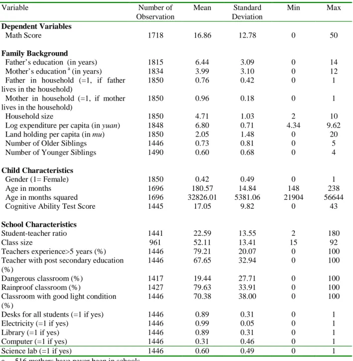
Table 1. Variable Definition and Summary Statistics Variable Number of Observation Mean Standard Deviation Min Max Dependent Variables Math Score 1718 16.86 12.78 0 50 Family Background

Father’s education (in years) 1815 6.44 3.09 0 14

Mother’s education a (in years) 1834 3.99 3.10 0 12

Father in household (=1, if father lives in the household)

1850 0.76 0.42 0 1

Mother in household (=1, if mother lives in the household)

1850 0.96 0.18 0 1

Household size 1850 4.71 1.03 2 10

Log expenditure per capita (in yuan) 1848 6.80 0.71 4.34 9.62

Land holding per capita (in mu) 1850 2.05 1.48 0 20

Number of Older Siblings 1446 0.73 0.81 0 5

Number of Younger Siblings 1490 0.60 0.68 0 4

Child Characteristics

Gender (1= Female) 1850 0.42 0.49 0 1

Age in months 1696 180.57 14.84 148 238

Age in months squared 1696 32826.01 5381.06 21904 56644

Cognitive Ability Test Score 1445 17.05 9.82 0 43

School Characteristics

Student-teacher ratio 1441 22.59 13.55 2 180

Class size 961 52.11 13.41 15 92

Teachers experience>5 years (%) 1446 79.21 20.07 0 100

Teacher with post secondary education (%)

1446 67.65 32.94 0 100

Dangerous classroom (%) 1417 19.44 27.71 0 100

Rainproof classroom (%) 1427 79.63 33.91 0 100

Classroom with good light condition (%)

1446 70.38 38.00 0 100

Desks for all students (=1 if yes) 1446 0.89 0.31 0 1

Electricity (=1 if yes) 1446 0.99 0.05 0 1

Library (=1 if yes) 1446 0.89 0.31 0 1

Computer (=1 if yes) 1446 0.31 0.46 0 1

Science lab (=1 if yes) 1446 0.60 0.49 0 1

a. 516 mothers have never been in schools.

b. Yuan is the Chinese currency. One dollar= 8.27 Yuan in 2004.

Table 2. First-Stage Regressions

Dependent variables (1) Cognitive

test score in 2000 (2) Cognitive test score in 2000 (3 )Log expenditure per capita Family Background: Father’s education 0.000 (0.079) -0.058 (0.073) 0.004 (0.005) Mother’s education 0.154 (0.111) 0.154 (0.099) 0.019*** (0.007) Father in household 0.999*b (0.526) 1.445*** (0.537) -0.025 (0.037) Mother in household -1.418 (1.390) -2.372 (1.544) 0.084 (0.109) Log expenditure per capitaa 1.219 (1.325) -- --

Landholding per capita 0.062 (0.164) 0.180 (0.207) 0.023 (0.014) Number of younger siblings 0.369 (0.507) 0.179 (0.402) -0.098 (0.028) Number of older siblings 0.445 (0.349) 0.304 (0.319) -0.032 (0.022) Log wealth per capita in 2000c -- 0.112 (0.255) 0.181*** (0.018) Father born in July 1958 -- 20.775*** (7.679) 0.325 (0.542) Mother born in December 1956 -- -15.601** (7.150) 0.229 (0.505)

Child Characteristics:

Female (1=female) -0.839 (0.698) -0.561 (0.697) 0.008 (0.049) Age in months -0.242 (0.313) -0.182 (0.302) 0.043** (0.021) Age in months squared 0.001 (0.001) 0.000 (0.001) -0.000** (0.000)

Gender Effects

Female×mother’s education 0.067 (0.136) -0.010 (0.131) 0.000 (0.001)

School Characteristics:

Student-teacher ratio 0.014 (0.013) Teachers with experience>5 years (%) -0.001 (0.012) Teacher with post secondary education (%) 0.047***(0.013) Dangerous classroom (%) 0.018* (0.010) Rainproof classroom (%) 0.004 (0.007) Classroom with good light condition (%) -0.009 (0.007) Desk for all students (=1 if yes) 1.767* (0.917) Electricity (=1 if yes) -2.834 (2.292) Library (=1 if yes) -0.994 (0.988) Computer (=1 if yes) -1.084 (0.757) Science lab (=1 if yes) 3.178***(0.657)

School Fixed Effects No Yes Yes

County Fixed Effects Yes no no

Sample size 1379 1408 1408

a. Robust standard errors are in parenthesis.

b.*** Significant at 1% level; ** significant at 5% level; * significant at 10% level. c. Household wealth is defined as value of fixed assets plus value of the house.