Technological University Dublin Technological University Dublin
ARROW@TU Dublin
ARROW@TU Dublin
Conference papers School of Accounting and Finance
2011
Volatility Analysis of Precious Metals Returns and Oil Returns
Volatility Analysis of Precious Metals Returns and Oil Returns
Lucia MoralesTechnological University Dublin, [email protected]
Bernadette Andreosso
Follow this and additional works at: https://arrow.tudublin.ie/buschaccon
Part of the Finance and Financial Management Commons
Recommended Citation Recommended Citation
Morales, Lucia and Andreosso, Bernadette: Volatility analysis of precious metals returns and oil returns. Working paper
This Working Paper is brought to you for free and open access by the School of Accounting and Finance at ARROW@TU Dublin. It has been accepted for inclusion in Conference papers by an authorized administrator of ARROW@TU Dublin. For more information, please contact [email protected],
[email protected], [email protected]. This work is licensed under a Creative Commons Attribution-Noncommercial-Share Alike 3.0 License
Volatility Analysis of Precious Metals Returns and Oil Returns: An ICSS Approach
Keywords: Stock Returns, Precious Metals Returns, GARCH modeling, ICSS algorithm.
JEL Codes: F, G.
Abstract
This study examines volatility persistence on precious metals returns taking into account oil returns and the three world major stock equity indices (Dow Jones Industrials, FTSE 100, and Nikkei 225) using daily data over the sample period January 1995- May 2008. We first determine when large changes in the volatility of each market returns occur, by identifying major global events that would increase the volatility of these markets; the Iterated Cumulative Sums of Squares (ICSS) algorithm helps identify the break points or sudden changes in the variance of returns in each market using the standardized residuals obtained through the GARCH(1,1) mean equation. Our main results identify a clear relationship between precious metals returns and oil returns, while the interaction between precious metals and stock returns seems to be an independent one. In relation to volatility persistence, the results are showing clear evidence of high volatility persistence between these markets.
1. Introduction
Already in the 1980s, research showed that increases in oil prices generated important effects in macroeconomic variables such as Gross National Product (GNP) (Hamilton 1983); Gilbert and Mork, 1984). In particular, Hamilton (1983) concluded that increases in oil prices are responsible for declines in real GNP; therefore, if oil prices play an important role in the economy, it is reasonable to expect the existence of correlations between oil prices and stock prices. Furthermore, given that investors use portfolio diversification as a strategy to minimize risk, the question arises as to what would the relation of these variables be with precious metals. The analysis of interlinkages between these variables is of high importance for investors. Consequently, the objective of this paper is to examine the effects of oil returns on precious metals markets, including the major financial markets (US-Dow Jones Industrial, Japan-Nikkei 225, and UK-FTSE 100) as a proxy to identify the strength of volatility persistence among these markets.
Ross (1989) argued that volatility is a measure of information flows; the analysis can be viewed as an investigation of the extent to which the rate of information flow in correlated across markets. The increasing integration of major financial markets throughout the world has generated interest in studying the transmission of financial markets shocks across markets (Ewing et al., 2002). It is important for financial markets participants to understand the volatility transmission mechanism across time and sector in order to facilitate optimal portfolio decisions. Thus, it is natural to be concerned with how information, and therefore, volatility, may flow from one market to another. Since index futures and options are an important tool that financial market participants can use in order to hedge against portfolio risk, and because the volatility of the index is a key determinant of futures and options valuation, it is important to understand what affects index volatility in those markets (Ewing et al., 2002).
A number of techniques have been used to model volatility. The autoregressive conditional heteroskedasticity (ARCH) model developed by Engle (1982), and later generalized by Bollerslev (1986) is the most popular method used for analyzing high-frequency financial time series data. Multivariate generalized autoregressive conditional heteroskedasticity (GARCH) models have been used to estimate the spillover effects and
volatility among different markets. It has been concluded that higher levels of conditional volatility in the past are associated with higher conditional volatility in the current period, which is associated with a volatility persistence value that is normally very close to one. A persistence value close to one is indicative of an integrated GARCH (IGARCH) process. The estimates of volatility persistence for each return series provide information about the extent to which post shocks and volatility matter in the construction of forecast of future conditional variance. The greater the persistence, the more weight should be given to recent observations of volatility, in terms of explaining future behavior of the variance. The volatility of the series will return to its conditional variance faster than would be the case when there is greater persistence. An alternative way of interpreting volatility persistence is to compute the half-life of an innovation or shock to the series, which will provide the days that return series take to lose half of it effect of the variance.
The recent situation in energy markets is an area of great interest for researchers when oil prices are soaring, and investors’ eyes tend to divert to commodities markets; therefore, we consider of interest the analysis of interactions between stock returns, oil returns and precious metals returns. The behavior of oil prices has received special attention, as the oil market has undergone structural transformations that have placed oil prices on a new high path, where new large consumers like China and India are playing an important role in the current market behavior. The rise in oil prices and the increase in oil price volatility have resorted to a wide list of drivers including strong demand (mainly from outside the OECD area), lack of spare capacity in upstream oil, distributional bottlenecks, OPEC supply response, geopolitical and weather shocks and the increasing role of speculators and traders in price information (Fattouh, 2007). The level of volatility in financial markets influence the corporate sector’s investment decisions and banks’ willingness and ability to extend credit facilities (Panetta et al., 2006). Therefore, it is important to know what impact changes in the volatility level might have on financial stability. The current economic situation reminds us the Bretton Woods system and brings to our minds the following questions:
a) Is it possible to be thinking about the importance of precious metals markets as
a key variable that could be used by governments to help in maintaining financial stability?
b) Precious metals are a source of increasing value; they are perceived as important and stable stores of value; why not use them to diversify portfolios?
Because risk management practices have improved considerably during the past years, financial institutions are better equipped to mitigate adverse effects in volatility. Financial factors affect volatility, investors’ risk tolerance, hedging strategies, structural changes in financial markets, etc. Financial derivatives for example have allowed market participant to price, unbundle and disperse risk throughout the financial system. Therefore, the analysis of equity markets, precious metals markets and oil prices deserves particular attention, due to the fact that these markets could be used in order to diversify the investors’ risk.
The hypothesis according to which stock markets are influenced by shocks in oil and precious metals markets, while precious metals markets are more stable and secure assets, is the core of this paper. It is possible to identify an independent behavior of precious metals regarding oil and equity markets during times of crises. This would be a highly valuable information for investors who would be able to design their investment strategies by taking into account the use of precious metals in the composition of their portfolios.
The remainder of the paper follows the ensuing structure. After a brief review of the pertinent literature in section 2, section 3 will describe the data and methodology that is used to detect changes in variance; in this section, the ICSS algorithm and the GARCH model are also discussed. Section 4 reports the main results and Section 5 concludes the analysis.
2. Literature Review
Huan, Masulis and Stoll (1996) studied the relationship between oil futures returns and stock returns during the 1980’s using a vector autoregressive (VAR) approach while controlling for interest rate effects, seasonality and other effects. Their conclusions were that oil futures returns are not correlated with stock market returns. Despite the frequently cited importance of oil for the economy, the authors found little evidence of such a link.
In fact, the lack of correlation suggests that oil futures, like other futures contracts, appear to have little correlation with stocks.
Aggarwal, Inclan and Leal (1999) examined the kind of events that caused shifts in the volatility of emerging stock markets, using an iterated cumulative sum squares (ICSS) algorithm to identify the points of shocks/sudden changes in the variance of returns in each market and how the long shift lasts. They identified that the October 1987 crash was the only global event during the period 1985-1995 that caused a significant jump in the volatility of several emerging stock markets. They examined ten of the largest emerging markets in Asia and Latin America. Their findings showed that the high volatility in emerging markets is marked by several shifts; the large changes in volatility seem to be related to important country-specific political, social and economic events. The number of changes in variance varies from country to country and they also depend on the data frequency; more change points are found with daily returns than with weekly or monthly returns.
Ewing, Malik and Ozfidan (2002) analyzed how volatility in the oil and natural gas sectors changed over time and across markets, examining the bivariate and univariate time-series properties of oil and natural gas index returns. They analyzed daily closing values for the period spanning over 01/04/1996 to 29/10/1999, and they found that volatility (conditional variance) in oil returns is directly affected by its own volatility, and by the volatility in the natural gas returns. Thus, they found significant direct and indirect transmissions effects of volatility in oil returns from the natural gas sector to the oil sector, but they did not find that volatility in oil returns was affected by shocks originating in either the oil sector or gas sector. Also, they did not find evidence of an indirect effect of shock in the natural gas sector on the oil sector. The behavior of natural gas return volatility differs from that of oil.
Al-Eisa, Al-Nsour, and Hammoudeh (2003) provided an institutional analysis of the financial valuations for the individual Gulf Cooperation Council (GCC) markets (Oman, Kuwait, Bahrain, Saudi Arabia and UAE). They examined whether any long-run relationship existed among these markets, using cointegration techniques and investigating the transmission of changes and volatility in oil prices, as represented by NYMEX oil futures prices, to the individual GCC stock markets, using the vector error
correction and GARCH models. They analyzed daily data for the GCC stock indices and the oil prices that cover the period 15/02/1994 to 25/12/2001. They found that the five GCC markets are strongly cointegrated; this means that they have many long-run relationships and that they co-move over time. Oil price volatility spillovers are significant in all the GCC markets; this volatility moves these markets in the same direction with the oil volatility at NYMEX, which means that should the oil prices become more volatile in NYMEX, the share prices in the GCC markets would feel this volatility.
Fernández (2004) examined the presence of structural breaks in volatility using two alternative approaches; the iterative cumulative sum of squares (ICSS) algorithm, and wavelet analysis. She looks at the effect of the outbreak of the Asian crisis and the terrorist attacks of September 2001, on emerging Asia and Latin America. She also analyzed North American and European stock markets. Her results show that the number of shifts detected by the two methods was substantially reduced when filtering out the data for conditional heteroskedasticity and serial correlation. In particular, for the filtered stock data, the ICSS algorithm did not find any volatility shifts over 1997-2002, whereas the wavelet analysis found evidence of volatility breakpoints at some given scales of the data and only for 1997-1998.
Zhang et al (2005) investigated the Shanghai stock exchange and analyzed how regulations affect volatility, applying a CUSUM type test on the SSE Composite Return Index as well as a Markow-Swithching ARCH model. They found that there was at least one break within the last decades and that the volatility of returns shows a significant reduction after the break. Their results show a main structural break happening mid 1997, which was consistent with the fact that some critical regulation improvements appear during that year.
Agren (2006) studied volatility spillovers from oil prices to stock markets within an asymmetric BEKK model, using weekly data on the aggregate stock markets of Japan, Norway, Sweden, the UK and the US. This study brings strong evidence of volatility spillovers for all stock markets with the exception of the Swedish one, where only weak evidence was found.
Wang and Moore (2007) analyzed sudden changes in volatility in the stock markets of new European Union members (Poland, The Czech Republic, Hungary, Slovakia and Slovenia), using weekly data over the sample period 1994-2006. They used the iterative cumulative sum squares (ICSS) algorithm and they found that sudden shifts are largely explained by domestic, economic and financial factors. This is consistent with Aggarwal et al. (1999).
The analysis of the literature shows that oil shocks and stock markets have received much attention, but that there is a lack of evidence regarding the interaction of these markets with precious metal markets. Our objective is to analyze volatility taking into account the ICSS algorithm to detect jumps in volatility using a GARCH (1,1) model. We intend to identify sudden changes in variance which will be used to correct the GARCH model. Therefore, we will be able to do a comparison between the results without taking into account the jumps and the results after the model is corrected for it.
3. Data and Methodology
The graphical analysis of oil prices (figure 1) from January 1995 to May 2008 shows how the crude oil prices have recently been following clear upward movement. Since the same behavior applies to Brent and WTI prices, we decide to use the Crude oil Brent prices in our analysis. In relation to the Dow Jones Industrial, FTSE 100 and Nikkei 225 indices, the graph for the last 13 years (figure 2) allow us to identify clearly the higher instability that exists in the main world equity markets. It is possible to appreciate pronounced downturns in the markets due to a number of factors, such as: the Asian Crisis (1997-1998), the terrorist attacks that affected the United States in September 2001, the dot.com bubble crisis covering roughly the period 1995 to 2001, the burst of the Internet Bubble during 2002 and the Chinese Correction during 2007 that saw?? the global stock market plunge in February 2007. The equity indexes reflect the clear instability of the markets during this particular time period, with special attention to the Nikkei 225 that seems to be the most volatile index of all. The oil and stock market prics seem to be reacting in a negatively manner to these major market crises. However, and according to figure 3, precious metals markets seem to follow a different pattern. They
seem to reflect an independent behavior; a clear upward trend is visible for gold and platinum and in a softer manner for silver prices after the Asian Crisis, a situation that has persisted until now.
3.1 Data
Our analysis focuses on the period 1 January 1995 to 25 April 2008.The data set
consists of daily closing values for the stock market indices for the major markets: US (Dow Jones Industrials), UK (FTSE-100) and Japan (Nikkei 225). In the case of the precious metals data, we took the US$/Troy ounce for gold, the London Free Market Platinum price in US$/Troy ounce, and the Zurich silver price in US$/kilogram, and finally we will use the oil prices taking into account the Crude Oil Brent. All our data series are from DataStream International, giving a total of 3480 observations for each series.
3.2Methodology
3.2.1 ICSS Algorithm
Inclan and Tiao (1994) designed the Iterative Cumulative Sums of Squares (ICSS) algorithm. This algorithm allows for detecting multiple break points in the variance in the case of time series. However, the literature has shown that the ICSS algorithms tend to overstate the number of actual breaks in variance (Fernández, 2004). Bacmann and Dubois (2002) pointed out that the behavior of the ICSS algorithm is questionable under the presence of conditional heteroskedasticity. They have shown that this problem can be solved by filtering the return series by a GARCH (1,1) model, and applying the ICSS algorithm to the standardized residuals. The present analysis will test for volatility shifts before and after filtering the data for conditional heteroskedascity and serial correlation for comparison purposes.
The ICSS algorithm assumes that the time series of interest has a stationary unconditional variance over an initial time period until a sudden break takes place. The unconditional variance is then stationary until the next sudden change occurs. This
process repeats itself through time, giving time series observations with a number of m breakpoints in the unconditional variance in n observations. To estimate the number of changes and the point of time of variance shifts, a cumulative sum of squared residuals is used. This is denoted as:
∑
= = k t t k C 1 2 ε (1)where k = 1,…..T, and {εt} is a series of uncorrelated random variables with zero
mean and unconditional variance 2
t
σ . The variance in each interval is denoted by 2
j σ , with j = 0,1,….., NT, where NT is the total number of variance changes in T
observations. By letting T T N < < < < <κ κ ... κ
1 1 2 be the set of breakpoints, the variance
then is defined as:
2 0 2 σ σt = 1<t<κ1 2 1 σ = κ1 <t<κ2 ... =σ12 t T T N < < κ (2)
The statistic DK is defined as follows,
T k C C D T k k = − with D0 = DT = 0 (3)
where CT is the sum of the squared residuals from the whole sample period. If there are no changes in variance over the whole sample period, Dk oscillates around zero; otherwise, if there are one or more shifts in variance, Dk will depart from zero. The critical values, which define the upper and lower limits for the drifts under the null hypothesis of stationary variance, determine significant changes in the variance of the series. If the maximum of the absolute value of the statistic Dk is greater than the critical value, the null hypotheses of no sudden changes is rejected. Let k* be the value of k at
which maxk¦Dk¦ is attained, and if maxk = (T/2)* Dk exceeds the critical values, then k* is taken as an estimate of the change point. The term (T/2)is used to standardize the distribution. The critical value of 1.358 is the 95th percentile of the asymptotic distribution of maxk = (T/2)* Dk . Therefore, upper and lower boundaries can be set
at ±1.358 in the Dk plot.
The ICSS is an iterative approach because the process must be repeated over subsamples to identify multiple change points. For example, if a point change is observed at τT, then, this point is used to partition the sample into two subsample, to τT and (τT+1)-T. The CSS is then estimated over both subsamples to identify additional point changes. The process is repeated until no new change points are identified.
3.2.2 The GARCH model
Once the change points in variance have been identified the GARCH model is estimated without and with sudden changes in variance. The standard GARCH (1,1) model is defined for the case without sudden changes as follow,
t t
t X e
Y =µ+δ1 −1+ (4)
where et It−1~ N(0, ht) and htis given by the variance equation:
1 1 − − + + = t t t e h h ω α β (5)
The GARCH(1,1) model with sudden changes and taking into account our variables, is as follow: t t t t X Z e Y =µ+δ1 −1+δ2 −1+ (6) 1 1 − − + + = t t t e h h ω α β (7) where:
Yt = Precious Metals Returns (Gold, Silver and Platinum)
Xt = Stock Markets Returns (Dow Jones Industrials, FTSE 100 and Nikkei 225) Zt = Crude Oil Brent,
1
− t t I
e ~ N(0, ht) and ht is given by the variance equation
1 1 1 1 +...+ + − + − + = n n t t t d D d D e h h ω α β (8)
where D1….Dn are the dummy variables, taking a value of 1 for each point of sudden change in the variance onwards, and of 0 otherwise. Given the modified GARCH model, this incorporates the regime shifts detected by the ICSS algorithms. The persistence of volatility, i.e. α + β is predicted to be smaller than that found by the conventional GARCH model. The GARCH (1,1) model would be adapted to our analysis, taking into account precious metals returns vs. stock market returns, and precious metals returns vs. oil returns. Therefore, the mean equation will be adjusted as follows:
yt n t i t i m t i t iSMx OR c PMy = +
∑
α +∑
λ +ε = − = − 1 1 0 (9)∑
∑
= − = − + + + + + = b i yt a i yt T n yt d D d D h h 1 2 1 1 1 1 1 1 1 0 ... β κ µ β (10)Following Kanas (2000) we use continuously compounded stock returns; we also applied the same procedure to work out the precious metals returns, calculated as the first
difference of the natural log. That is: if S= Stock Prices, then
( )
(
s)
t s
t
t P P
S = ln −ln −1 .
Similarly, if PM= Precious Metals Prices, then
(
)
(
PM)
t PM
t
t P P
PM = ln − ln −1 ; and if OR =
Oil Returns, then
(
)
(
OR)
t OR t OR t P P OR = ln −ln −1 .
Where PMy = Gold, Silver, Platinum.
SM = Dow Jones Industrials, FTSE 100, Nikkei 225. OR = Crude Oil Brent.
4. Empirical Results
4.1 Descriptive Statistics
The descriptive statistics of precious metals returns (table 1) show a common trend. The three markets present positive and small mean values. The standard deviation indicates that the gold market is the less volatile with a coefficient of 0.89 per cent; the silver returns are the most volatile with a coefficient of 1.73 per cent, and platinum shows a standard deviation equal to 1.36 per cent. In the case of stock returns, the situation is slightly different; our results show that the mean values for the Down Jones and FTSE 100 are positive and small. This is consistent with the results that we got for the precious metals returns, while the results for the Nikkei 225 are showing a negative mean, explained by the negative performance during the Japanese ‘lost decade’. The analysis of the stock returns volatility shows that overall the Nikkei 225 is the most volatile stock returns series, with a daily standard deviation of 1.39 per cent. Standard deviations are 1.03 per cent and 1.07 per cent in the case of the Dow Jones and FTSE 100 respectively. The analysis of oil returns represented by the Brent returns shows a small positive mean value. The volatility analysis shows that oil returns are the most volatile market in relation to stock returns and precious metals returns, with a coefficient of 2.24 per cent. The skewness and kurtosis coefficients indicate that stock returns, precious metals returns and oil returns are leptokurtic and negatively skewed regarding the normal distribution, which Caporale et al.. (2002) note is a common finding for stock returns. The Jarque-Bera test also rejects the hypothesis that stock returns, precious metals returns and oil returns are normally distributed in all the cases.
Table 1 here
4.2 Unit Roots Tests
The results from the ADF tests are given in table 2. The values of the test statistics indicate that we can reject the null hypothesis of the existence of a unit root in
levels for all variables during all periods indicating that all series are I(0).1 Given that all variables are integrated of the same order, (i.e. I(0)), we proceed directly to perform our volatility analysis using GARCH (1,1) modeling.
Table 2 here
4.3. ICSS Break Points
The ICSS algorithm results are presented in tables 3 to 5. First we decide to run the algorithm using the original series to work out the number of break points. As can be seen in table 3 and table 4, the number of sudden changes in volatility is quite high. The main problem is the non existence of common break points between the sudden changes in volatility for the different indices; this is a problem when introducing all the break points in the variance equation. Another problem is the number of observations that should be considered as a breakpoint. If we consider appropriate to eliminate an important number of observations from the data set, this action could be generating by its own a break point, due to the fact that there will be an important gap between the observation that generated the jump and the last observation included in the sample, where it is considered that the volatility shock disappeared. In order to solve this problem, we decided to implement the GARCH(1,1) model using the mean equation for each of the precious metals under analysis (equation 9). The results are presented in table 5 and in figures 4 to 12. It is possible to appreciate how the numbers of sudden changes in volatility have been reduced for each of the precious metals equation, and also how we solve the problem of getting different numbers and days on volatility jumps.
Table 3-5 here
1
The LMF test results indicated that the ADF tests were free from serial correlation; for the sake of brevity, we do not show the test results here.
4.4 Volatility Results
The analyses of the coefficients for the volatility persistence are presented in tables 6 to 8. The parameter conditions constraints are:β0 ≥0, 1≥β1 ≥0, 1≥κ1 ≥0
) 1
(β1+κ1 ≤ . These constraints are applied to the parameters to enforce stationarity and a positive conditional variance. Volatility persistence will be measured through the sum of the following coefficients for each equation(β1 +κ1 ≤1). The GARCH(1,1) results are obtained through two main regressions:
a) First of all we run a normal GARCH(1,1) model, represented by either equation
(6) or (9) which will give us the variance output represented by equation (7).
b) Then we run a GARCH(1,1) model, represented by either equation (6) or (9),
but in this case the variance will be adjusted to the breakpoints found by the ICSS algorithm in order to compare the volatility persistence results; the variance output is represented by equation (10).
Tables 6-8 here
Regarding the returns-generating process (the results of which are presented through tables 6 to 8) we can draw the following conclusions.
4.4.1 Gold Analysis
The analysis of the GARCH(1,1) model for the Gold equation (table 6) shows a significant negative relation between gold returns and the Dow Jones returns, a positive significant coefficient in the case of Gold-FTSE 100, while the coefficient is insignificant regarding the Nikkei 225. The results for the GARCH(1,1) with dummies show an insignificant relationship between the Gold returns and the three stock markets returns. The results also show that there is a significant positive relationship between the gold market returns and the Brent returns; both the GARCH(1,1) and the GARCH(1,1) with dummies show a positive significant relation between precious metal returns and oil returns, with all the coefficients being significant at the 1% and 5% significance levels.
This situation reflects that, in general when the oil markets are appreciating there is a trend of increasing returns for the gold market.
Examining the variance estimates we can appreciate that for both models the GARCH parameter for volatility persistence is moving between 0.75 (lowest value) to 0.95 (highest value). With regard to volatility persistence, the sum of the GARCH coefficients is close to 1 implying extreme persistence in volatility for both GARCH models.
4.4.2 Silver Analysis
The analysis of the GARCH(1,1) model for the Silver equation (table 7) shows an insignificant relation between silver returns and the Dow Jones returns, while a positive significant coefficient is found in the case of Silver-FTSE 100, and Silver-Nikkei 225. These results are confirmed by the output obtained from the GARCH(1,1) with dummies. The results also show that there is a significant positive relationship between the silver market returns and the Brent returns; both the GARCH(1,1) and the GARCH(1,1) with dummies models show a positive significant relationship between silver precious metal returns and oil returns, with all the coefficients being significant at the 1% and 5% significance levels. This situation reflects that, in general when the oil markets are appreciating there is a trend of increasing returns for the silver market, a result consistent with the findings for the gold market.
Examining the variance estimates we can appreciate that for both models the GARCH parameters for volatility persistence are positive and significant with all the coefficients moving between the two extreme values of 0.82 and 0.94.
4.4.3 Platinum Analysis
GARCH(1,1) results for the Platinum equation (table 8) show a significant positive relationship between platinum returns and both the Dow Jones returns and the Nikkei 225 returns, as well as an insignificant coefficient in the case of Platinum-FTSE 100. These results are corroborated with results from the GARCH(1,1) with dummies model. Our findings also show that there is a significant positive relationship between the platinum
market returns and the Brent returns at the 1 per cent level. Both the GARCH(1,1) and the GARCH(1,1) with dummies show a positive and significant relationship between precious metal returns and oil returns, with all the coefficients being significant at the 1% level. This situation reflects that, in general when the oil markets are appreciating there is also a trend of increasing returns in the platinum market.
Examining the variance estimates, we can appreciate that for both models, the GARCH parameter for volatility persistence is moving between 0.85 and 0.86, implying that volatility tend to last in these markets.
With regard to volatility persistence the coefficients for each of the equations are significant, with the characteristic of a reduction in the magnitude of the GARCH coefficients for the GARCH with dummies. The sum of the GARCH coefficients is close to 1 in all the cases implying extreme persistence in volatility for both GARCH models, results that are influenced by the volatility persistence that characterised equity markets over the period under review. Overall, the results from the GARCH model with dummies show a reduction in the magnitude of the coefficients, implying that the level of volatility persistence tends to be corrected. The results also show a weak evidence regarding the influence of stock returns on precious metals returns, while the oil market seems to have a direct effect on precious metals markets.
4.5 Standardized Residual
The diagnostic tests on the standardised residuals for both GARCH models2 indicate that in the case of the Jarque-Bera test we reject the hypothesis that the residuals are normally distributed in all the cases, hence justifying the use of the Bollerslev-Woolridge robust t-statistics. The Ljung-Box statistics for all metals equations indicate that there are no residual linear or non linear dependencies in most of the cases. Finally, to check the validity of the assumption of constant correlation adopted in the estimation of the models (Kanas, 2000), the LB statistics for the cross products of the standardised residuals from the precious metals returns equation are calculated and these statistics indicated that the assumption of constant correlation over time can be accepted in almost
all the cases. These exceptions are normally corrected after increasing or decreasing the number of lags in the test.
The ARCH-LM residual test results show that overall the variance equation for the GARCH model is correctly specified, as we reject the null hypothesis of remaining ARCH effects in the equation in almost all the cases. This problem is corrected after increasing or decreasing the number of lags used in the estimation. The test results show that the variance equation is correctly specified as well for the GARCH dummy model, as we reject the null hypothesis in almost all the cases.
5. Conclusions
Sudden increases in oil prices (as in the 1970s and 2000s) lead to portfolio diversification, as a strategy to minimize risk. Analyzing the relationship between oil prices, stock prices and precious metals prices is of high importance for investors. This represents the prime motivation of this study. We have used the Inclan and Tiao (1994) iterated cumulative sums of squares (ICSS) algorithm to identify sudden shifts in volatility in precious metals markets (Gold, Platinum and Silver), three major stock markets (Dow Jones Industrials, FTSE 100, and Nikkei 225) and oil prices (Crude Oil Brent). In our analysis, we first implemented the ICSS algorithm to identify sudden changes in variance using each series individually. Our results have shown a great number of breakpoints and inconsistencies among each of the series under analysis in relation to identifying common points that allow to find the relevant dummy variables to be included in the GARCH model so as to analyze volatility persistence. Therefore, and in order to avoid the overestimation of breakpoints detected by the ICSS algorithm, we decided to use the GARCH(1,1) model to obtain the standardized residuals. The model is used to estimate the relevant volatility jumps that would be identified as the main dummy variables to analyze the relationship between precious metals returns, stock returns, and oil returns.
We first used the normal GARCH(1,1) model and afterwards we also used the ICSS-GARCH extended model which incorporates the volatility breakpoints identified by the ICSS algorithm. Our main results show that there is a significant positive relationship
between precious metals market returns and the Brent returns; both the GARCH(1,1) and the GARCH(1,1) with dummies show a positive significant relationship between precious metal returns and oil returns. This situation reflects that, in general when the oil markets are appreciating there is a trend of increasing returns for the gold market. In relation to the equity markets, most of the coefficients appear to be insignificant. This means that shocks in equity markets do not tend to generate major effects in precious metals markets. We also found that all the coefficients for the ICSS model are statistically significant; a characteristic is that the volatility persistence coefficient tends to reduce its value after the inclusion of the dummy variables that correct the results for sudden shifts in conditional volatility.
Our results are of importance to investors due to the fact that stock markets are influenced by shocks in oil and precious metals markets, while precious metals markets are seen as more stable and secure assets. Therefore, the independent behavior of precious metals regarding oil and equity markets during times of crises, and the constant upward trend that these markets are facing represent a highly valuable piece of information for investors who can design their investment strategies by taking into account the use of precious metals in the composition of their portfolios. Our initial results bring some useful evidence on the important implications derived from the new role that precious metals markets could exercise for investors. This is consequently a topic worthy of future research. Subsequent studies could use EGARCH modeling and also data with different frequencies (weekly and monthly); this would provide more evidence on the real importance of precious metals markets.
6. References
Aggarwal, R., Inclan, C. and Leal, R. (1999) Volatility in emerging stock markets, Journal of Financial and Quantitative Analysis 34, 33-55.
Agren, M., (2006) Does Oil Price Uncertainty Transmit to Stock Markets? Uppsala Universitet, Working Paper No.23.
Alberola, R., (2007) Estimating Volatility Returns Using ARCH Models. An Empirical Case: The Spanish Energy Market, Lecturas de Economia 66, 251-276.
Al-Eisa, E., Hammoudeh, S., Al-Nsour, R. (2003) Links and Volatility Transmisión Among the GCC Stock Markets and the NYMEX Oil Futures, Topics in Middle Eastern and North African Economies, Electronic Journal, Volume 5, Middle East Economic Association and Loyola University, Chicago.
Bollerslev. T. (1986) Generalized Autoregressive Conditional Heteroscedasticity, Journal of Econometrics 31, 307-327.
Ewing, B.T., Malik, F., Ozfidan, O., (2002) Volatility Transmission in the Oil and Natural Gas Markets, Energy Economics 24, 525-538.
Engle, R. F. (1982) Autorregresive Conditional Heteroskedasticity with estimates of the variance of UK inflation, Econometrica, 50, 987-1008.
Fang, W., Miller, S., Lee, C., (2007) Cross-Country Evidence on Output Growth Volatility: Non-stationary Variance and Garch Models. University of Connecticut. Workin Paper 2007-20.
Fattouh, B., (2007) The Drivers of Oil Prices: Te Usefulness and Limitations of Non-Structural model, the Demand-Supply Framework and Informal Approaches, Oxford Institute for Energy Studies, Working Paper 32.
Fernandez, V., (2004) Dectection of Breakpoints in Volatility. Estudios de Administracion, vol 11. No.1.
Gilbert, R.J., and Mork, K. A. (1984) Will Oil Markets Tighten Again? A survey of Policies to Manage Possible Oil Supply Disruption. Journal of Policy Modelin 6, pp. 111-142.
Hamilton, J.D. (1983) Oil and the Macroeconomy since World War II. Journal of Political Economy 91, pp. 228-248.
Huan, R., Masulis, R., and Stoll, H., (1996) Energy Shocks and Financial Markets, Journal of Futures Markets 16(1).
Inclan, C. and Tiao, G.C. (1994) Use of cumulative sums of squares for retrospective detection of changes of variance, Journal of the American Statistical Association, 89, 913-923.
Long, T.L., (2008) Empirical Analysis of Stock Return Volatility with Regime Change Using GARCH model: The case of Vietnam Stock Market. Vietnam Development Forum. Working Paper 084.
Malik, F., (2003) Sudden changes in variance and volatility persistence in foreign exchange markets. Journal of Multinational Financial Management 13, 217-230. Mansur, I., Cochran, S., Shaffer, D., (2007) Foreign Exchange Volatility Shifts and
Futures Hedging: An ICSS-GARCH Approach, Review of Pacific Basin Financial Markets Policies, Vol. 10, No.3, 349-388.
Panetta, F. et al., (2006) The Recent Behavior of Financial Market Volatility, Bank for International Settlements, No.29.
Ross, S., (1989) Information and Volatility: The No-Arbirtrage Martingale Approach to Timing and Resolution Irrelevancy. Journal of Finance 44, pp. 1-17.
Wang, P., Moore, T., (2007) Sudden changes in volatility: The case of five central European Stock Markets.
Zhang, D., Dickinson, D., Barassi, M., (2005) Volatility Switching in Shanghai Stock Exchange: Does regulation help reduce volatility?. The University of Birmingham Working Papers.
7. A p p en d ix F ig u re 1 : C ru d e B re n t O il & C ru d e O il – W T I S p o t C u sh in g O il P r ic e s 0 20 40 60 80 1 0 0 1 2 0 1 4 0 01/02/1995 10/10/1995 17/7/1996 24/4/1997 30/1/1998 11/09/1998 17/8/1999 24/5/2000 03/01/2001 12/07/2001 16/9/2002 24/6/2003 31/3/2004 01/06/2005 14/10/2005 24/7/2006 05/01/2007 02/06/2008 W T I B R F ig u re 2 : D o w J o n es , F T S E -1 0 0 & N ik k ei 2 2 5 S t o c k P r ic e s 0 5 0 0 0 1 0 0 0 0 1 5 0 0 0 2 0 0 0 0 2 5 0 0 0 01/02/1995 09/06/1995 05/10/1996 14/1/1997 18/9/1997 25/5/1998 27/1/1999 10/01/1999 06/06/2000 02/08/2001 15/10/2001 19/6/2002 21/2/2003 28/10/2003 07/01/2004 03/07/2005 11/09/2005 14/7/2006 20/3/2007 22/11/2007 D J F T N K F ig u re 3 : G o ld , S ilv er a n d P la tin u m P r e c i o u s M e t a l s P r i c e s 0 ,0 0 5 0 0 ,0 0 1 0 0 0 ,0 0 1 5 0 0 ,0 0 2 0 0 0 ,0 0 2 5 0 0 ,0 0 01/02/1995 19/10/1995 08/06/1996 23/5/1997 03/11/1998 28/12/1998 14/10/1999 08/01/2000 18/5/2001 03/06/2002 23/12/2002 10/09/2003 27/7/2004 13/5/2005 03/01/2006 18/12/2006 10/04/2007 G D S I P L
Table 1: Descriptive Statistics
GOLD SILVER PLATINUM DOW FTSE NIKKEI BRENT
Mean 0.000243 0.000356 0.000445 0.000349 0.000198 -0.000101 0.000570
Std. Dev. 0.008931 0.017309 0.013689 0.010342 0.010788 0.013954 0.022474
Skewness -0.105000 -0.534531 -0.627836 -0.247420 -0.198963 -0.084421 -0.113218
Kurtosis 10.204 1.073 1.785 7.452 6.113 5.161 6.172
Jarque-Bera 7519 8837 32155 2905 1426 680 1464
Table 2: Unit Roots
GOLD SILVER PLATINUM DOW FTSE NIKKEI BRENT
ADF -58.18* -13.04* -13.13* -43.14* -14.71* -43.77* -21.87*
*1% significance level.
Table 3: Precious Metals Break Points* Gold Series Silver Series Platinum Series May 9, 1995 December 29, 1995 March 1, 1996 December 31, 1996 March 4, 1997 May 16, 1997 July 2, 1997 October 9, 1998 September 17, 1999 October 5, 1999 December 8, 1999 February 2, 2000 February 8, 2000 July 19, 2000 January 26, 2001 March 13, 2001 May 17, 2001 September 7, 2001 September 18, 2001 January 31, 2002 August 8, 2002 January 31, 2003 July 22, 2004 December 5, 2005 May 5, 2006 October 3, 2006 November 1, 2007 March 3, 2008 March 17, 2008 March 29, 1995 May 9, 1995 October 2, 1995 December 2, 1996 December 8, 1997 December 16, 1997 May 29, 1998 March 15, 1999 September 27, 1999 September 30, 1999 June 21, 2000 January 1, 2001 May 14, 2001 August 14, 2002 July 14, 2003 January 2, 2004 April 12, 2004 May 10, 2004 March 8, 2005 December 5, 2005 April 14, 2006 June 14, 2006 October 3, 2006 February 25, 2008 March 19, 2008 March 27, 1995 May 9, 1995 March 4, 1996 February 11, 1997 May 28, 1997 August 24, 1998 September 21, 1998 December 10, 1998 December 18, 1998 January 22, 1999 January 27, 1999 September 23, 1999 November 18, 1999 January 26, 2000 February 29, 2000 August 7, 2000 July 13, 2001 October 16, 2001 June 3, 2001 April 9, 2004 May 17, 2004 December 7, 2004 October 28, 2005 May 5, 2006 June 19, 2006 October 30, 2006 November 16, 2006 November 21, 2006 March 14, 2007 September 26, 2007 November 15, 2007 January 22, 2008
*Break points calculated using the ICSS algorithm for each of the series. The ICSS algorithm for the individual series overestimate the number of points where sudden changes in volatility occur.
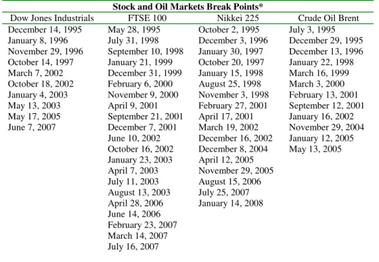
Table 4: Stock and Oil Markets Break Points
Stock and Oil Markets Break Points*
Dow Jones Industrials FTSE 100 Nikkei 225 Crude Oil Brent
December 14, 1995 January 8, 1996 November 29, 1996 October 14, 1997 March 7, 2002 October 18, 2002 January 4, 2003 May 13, 2003 May 17, 2005 June 7, 2007 May 28, 1995 July 31, 1998 September 10, 1998 January 21, 1999 December 31, 1999 February 6, 2000 November 9, 2000 April 9, 2001 September 21, 2001 December 7, 2001 June 10, 2002 October 16, 2002 January 23, 2003 April 7, 2003 July 11, 2003 August 13, 2003 April 28, 2006 June 14, 2006 February 23, 2007 March 14, 2007 July 16, 2007 October 2, 1995 December 3, 1996 January 30, 1997 October 20, 1997 January 15, 1998 August 25, 1998 November 3, 1998 February 27, 2001 April 17, 2001 March 19, 2002 December 16, 2002 December 8, 2004 April 12, 2005 November 29, 2005 August 15, 2006 July 25, 2007 January 14, 2008 July 3, 1995 December 29, 1995 December 13, 1996 January 22, 1998 March 16, 1999 March 3, 2000 February 13, 2001 September 12, 2001 January 16, 2002 November 29, 2004 January 12, 2005 May 13, 2005
*Break points calculated using the ICSS algorithm for each of the series. The ICSS algorithm for the individual
series overestimate the number of points where sudden changes in volatility occur, same situation was found in the case of the precious metals indices. Another problem is that each series are presenting a different number of break points that happened at different days during the period of analysis, therefore and in order to get a common number of break points we we decide to use the standardized residuals of the GARCH(1,1) (equation 9) that will allow us to get the appropriate number of break points to improve our variance equation (equation 10).
Table 5: GARCH(1,1) Residuals Break Points*
Gold-Dow Jones Ind.-Brent Gold-FTSE 100-Brent Gold-Nikkei 225-Brent
March 28, 1995 (obs.63) March 29, 1995 (obs.64) December 30, 1995 (obs.522) May 28, 2001(obs.1672) September 5, 2001(obs.1744) September 12, 2001(obs.1749) March 28, 1995 (obs.63) March 29, 1995 (obs.64) August 15, 1995 (obs.163) November 2, 1995 (obs.220) February 29,1996 (obs.305) July 31, 1996 (obs.414) December 12, 1996 (obs.522) March 28, 1995 (obs.63) March 29, 1995 (obs.64) December 30, 1995 (obs.522) May 28, 2001 (obs.1672) September 5, 2001 (obs.1744) September 10, 2001 (obs.1747)
Silver-Dow Jones Ind.-Brent Silver-FTSE 100-Brent Silver-Nikkei 225-Brent
September 29, 1999 (obs.1239) May 7, 2001 (obs.1657) July 7, 2003 (obs.2222) September 29, 1999 (obs.1239) July 5, 2001 (obs.1657) July 4, 2003 (obs.2221) September 29, 1999 (obs.1239) May 7, 2001 (obs.1657) July 7, 2003 (obs.222)
Platinum-Dow Jones Ind.-Brent Platinum-FTSE 100-Brent Platinum-Nikkei 225-Brent
May 31, 1996 (obs.371) February 10, 1997 (obs.552) August 27, 2002 (obs.1998) May 31, 1996 (obs.371) February 10, 1997 (obs.552) August 27, 2002 (obs.1998) May 31, 1996 (obs.371) February 10, 1997 (obs.552) August 27, 2002 (obs.1998)
*The ICSS algorithm using the GARCH(1,1) standardized residuals have the advantage of reducing the number of
Points where sudden changes in volatility occurs and also have the quality of providing a common break point for our mean equation, allowing us to reduce the number of dummy variables that should be introduce in the GARCH(1,1) variance equation..
GARCH(1,1) Results Table 6: Gold Analysis
Gold-Dow Jones Industrial-Brent Gold-FTSE 100-Brent Gold-Nikkei 225-Brent
GARCH (1,1)
GARCH(1,1)
with dummies GARCH (1,1)
GARCH(1,1)
with dummies GARCH (1,1)
GARCH(1,1) with dummies c0 0.0000 (0.789) 0.0000 (0.665) -0.0001 (0.550) 0.0001 (0.682) -0.0001 (0.643) -0.0001 (0.275) α -0.0349** (0.015) -0.0042 (0.762) 0.0351* (0.009) -0.0083 (0.688) 0.0115 (0.213) 0.0062 (0.480) λ 0.0209* (0.000) 0.0149** (0.011) 0.0146** (0.012) 0.0287* (0.001) 0.0145** (0.013) 0.0229* (0.000) β0 0.0000** (0.018) 0.0000** (0.011) 0.0000** (0.021) 0.0000* (0.000) 0.0000** (0.011) 0.0000* (0.000) β1 0.0505* (0.000) 0.0535* (0.000) 0.0515* (0.000) 0.1746* (0.000) 0.0527* (0.000) 0.1284* (0.000) κ1 0.9510* (0.000) 0.9483* (0.000) 0.9504* (0.000) 0.7582* (0.000) 0.9491* (0.000) 0.8567* (0.000) β1+ κ1 1.00 1.00 1.00 0.932 1.00 0.984
*1% significance level, **5% significance level and ***10% significance level.β1 is the coefficient for previous shocks and κ1 is the
coefficient for persistence.
Table 7: Silver Analysis
Silver-Dow Jones Industrial-Brent Silver-FTSE 100-Brent Silver-Nikkei 225-Brent
GARCH (1,1)
GARCH(1,1)
with dummies GARCH (1,1)
GARCH(1,1)
with dummies GARCH (1,1)
GARCH(1,1) with dummies c0 0.0000 (0.885) 0.0000 (0.910) 0.0000 (0.905) 0.0000 (0.926) 0.0000 (0.941) 0.0004 (0.194) α 0.0135 (0.539) 0.0074 (0.728) 0.0542** (0.011) 0.0427** (0.043) 0.0570* (0.000) 0.0661* (0.000) λ 0.0333* (0.000) 0.0317* (0.001) 0.0323* (0.001) 0.0340* (0.000) 0.0300* (0.002) 0.0635* (0.000) β0 0.0000* (0.001) 0.0000* (0.008) 0.0000* (0.002) 0.0002 (0.314) 0.0000* (0.002) 0.0000* (0.000) β1 0.0579* (0.000) 0.0562* (0.000) 0.0572* (0.000) 0.0836* (0.000) 0.0580* (0.000) 0.1386* (0.000) κ1 0.9393* (0.000) 0.9414* (0.000) 0.9404* (0.000) 0.9093* (0.000) 0.9394* (0.000) 0.8245* (0.000) β1+ κ1 0.996 0.997 0.997 0.992 0.997 0.962
*1% significance level, **5% significance level and ***10% significance level.β1 is the coefficient for previous shocks and κ1 is the
Table 8: Platinum Analysis
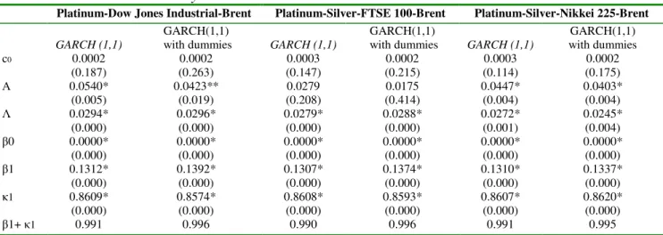
Platinum-Dow Jones Industrial-Brent Platinum-Silver-FTSE 100-Brent Platinum-Silver-Nikkei 225-Brent
GARCH (1,1)
GARCH(1,1)
with dummies GARCH (1,1)
GARCH(1,1)
with dummies GARCH (1,1)
GARCH(1,1) with dummies c0 0.0002 (0.187) 0.0002 (0.263) 0.0003 (0.147) 0.0002 (0.215) 0.0003 (0.114) 0.0002 (0.175) Α 0.0540* (0.005) 0.0423** (0.019) 0.0279 (0.208) 0.0175 (0.414) 0.0447* (0.004) 0.0403* (0.004) Λ 0.0294* (0.000) 0.0296* (0.000) 0.0279* (0.000) 0.0288* (0.000) 0.0272* (0.001) 0.0245* (0.004) β0 0.0000* (0.000) 0.0000* (0.000) 0.0000* (0.000) 0.0000* (0.000) 0.0000* (0.000) 0.0000* (0.000) β1 0.1312* (0.000) 0.1392* (0.000) 0.1307* (0.000) 0.1374* (0.000) 0.1310* (0.000) 0.1337* (0.000) κ1 0.8609* (0.000) 0.8574* (0.000) 0.8608* (0.000) 0.8593* (0.000) 0.8607* (0.000) 0.8620* (0.000) β1+ κ1 0.991 0.996 0.990 0.996 0.991 0.995
*1% significance level, **5% significance level and ***10% significance level.β1 is the coefficient for previous shocks and κ1 is the