Text Databases
Panagiotis G. Ipeirotis
Submitted in partial fulfillment of the requirements for the degree
of Doctor of Philosophy
in the Graduate School of Arts and Sciences
COLUMBIA UNIVERSITY 2004
Classifying and Searching Hidden-Web Text Databases
Panagiotis G. Ipeirotis
The World-Wide Web continues to grow rapidly, which makes exploiting all available information a challenge. Search engines such as Google index an unprecedented amount of information, but still do not provide access to valu-able content in text databases “hidden” behind search interfaces. For example, current search engines largely ignore the contents of the Library of Congress, the US Patent and Trademark database, newspaper archives, and many other valuable sources of information because their contents are not “crawlable.” However, users should be able to find the information that they need with as little effort as possible, regardless of whether this information is crawlable or not. As a significant step towards this goal, we have designed algorithms that support browsing and searching —the two dominant ways of finding information on the web— over “hidden-web” text databases.
To support browsing, we have developedQProber, a system that automatically categorizes hidden-web text databases in a classification scheme, according to their topical focus. QProbercategorizes databases without retrieving any docu-ment. Instead, QProber uses just the number of matches generated from a small number of topically focused query probes. The query probes are au-tomatically generatedusing state-of-the-art supervised machine learning tech-niques and are typically short. QProber’s classification approach is sometimes orders of magnitude faster than approaches that require document retrieval. To support searching, we have developed crucial building blocks for construct-ing sophisticated metasearchers, which search over many text databases at once through a unified query interface. For scalability and effectiveness, it is crucial for a metasearcher to have a gooddatabase selectioncomponent and send queries only to databases with relevant content. Usually, database se-lection algorithms rely on statistics that characterize the contents of each da-tabase. Unfortunately, many hidden-web text databases are completely au-tonomous and do not report any summaries of their contents. To build con-tent summaries for such databases, we extract a small, topically focused doc-ument sample from each database during categorization and use it to build the respective content summaries. A potential problem with content sum-maries derived from document samples is that any reasonably small sample will suffer from data sparseness and will not contain many words that appear in the database. To enhance the sparse samples and improve the database selection decisions, we exploit the fact that topically similar databases tend to have similar vocabularies, so samples extracted from databases with similar topical focus can complement each other. We have developed two database se-lection algorithms that exploit this observation. The first algorithm proceeds hierarchically and selects first the best category for a query and then sends the query to the appropriate databases in the chosen category. The second
data-content summaries with category-specific words. The shrinkage-enhanced summaries characterize the database contents better than their “unshrunk” counterparts do, and in turn help produce significantly more relevant data-base selection decisions and overall search results.
Content summaries of static databases do not need to change over time. How-ever, databases are rarely static and the statistical summaries that describe their contents need to be updated periodically to reflect content changes. To understand how real-world databases change over time and how these changes propagate to the database content summaries, we studied how the content summaries of152 real web databases changed every week, for a pe-riod of52 weeks. Then, we used “survival analysis” techniques to examine which parameters can help predict when the content summaries need to be updated. Based on the results of this study, we designed algorithms that analyze various characteristics of the databases and their update history to predict when the content summaries need to be modified, thus avoiding over-loading the databases unnecessarily.
In summary, this thesis presents building blocks that are critical to enable access to the often valuable contents of hidden-web text databases, hopefully approaching the goal of making access to these databases as easy and efficient as over regular web pages.
1 Introduction 1
2 Classifying Hidden-Web Text Databases 5
2.1 Classification of Text Databases . . . 7
2.1.1 Hierarchical Classification Schemes . . . 7
2.1.2 The Text Database Classification Task . . . 8
2.2 Classifying Databases through Probing . . . 11
2.2.1 Training a Document Classifier . . . 11
2.2.2 Defining Query Probes from a Rule-Based Document Classifier . . . 12
2.2.3 Extracting Query Probes from Numerically Parameter-ized Document Classifiers . . . 15
2.2.4 Adjusting Probing Results . . . 18
2.2.5 Using Probing Results for Classification . . . 20
2.3 Experimental Setting . . . 22
2.3.1 Data Sets . . . 22
2.3.2 Techniques for Comparison . . . 24
2.3.2.1 QProber Variations . . . 24
2.3.2.2 Document Sampling (DS) . . . 24
2.3.2.3 Title-based Querying (TQ) . . . 25
2.3.3 Evaluation Metrics . . . 26
2.4 Experimental Results . . . 28
2.4.1 Tuning QProber and DS . . . 28
2.4.2 Results over the Controlled Databases . . . 30
2.4.3 Results over the Web Databases . . . 39
2.5 Beyond Hidden-Web Text Databases . . . 43
2.6 Further Discussion . . . 46
2.7 Conclusions . . . 47
3 Constructing Database Content Summaries 49 3.1 Background . . . 51
3.1.1 Database Selection Algorithms . . . 51
3.1.2 Uniform Probing for Content Summary Construction . 52 3.2 Focused Probing for Content Summary Construction . . . 54
3.3 Estimating Absolute Document Frequencies . . . 57
3.4 Improving Content Summaries using Shrinkage . . . 60
3.4.1 Overview of our Approach . . . 60
3.5.1 Data Sets . . . 67
3.5.2 Techniques for Comparison . . . 68
3.5.2.1 Sampling Algorithms . . . 68
3.5.2.2 Shrinkage and Frequency Estimation . . . 69
3.6 Experimental Results . . . 69
3.6.1 Effect of Sampling Algorithm . . . 70
3.6.2 Effect of Shrinkage . . . 77
3.6.2.1 Relationship between Content Summaries and Categories . . . 79
3.6.2.2 Properties of Shrinkage-based Content Summaries 80 3.7 Conclusions . . . 84
4 Classification-Aware Database Selection 85 4.1 Exploiting Topic Hierarchies for Database Selection . . . 86
4.2 Improving Database Selection using Shrinkage . . . 90
4.3 Experimental Setting . . . 92
4.3.1 Data Sets . . . 92
4.3.2 Techniques for Comparison . . . 92
4.4 Experimental Results . . . 106
4.5 Conclusion . . . 118
5 Updating Database Content Summaries 123 5.1 Studying Content Changes of Real Text Databases . . . 124
5.1.1 Data for our Study . . . 124
5.1.2 Measuring Content Summary Change . . . 125
5.2 Predicting Content Summary Change Frequency . . . 135
5.2.1 Survival Analysis . . . 135
5.2.2 Cox Proportional Hazards Regression Model . . . 136
5.2.3 Using Cox Regression to Model Content Summary Changes137 5.3 Scheduling Updates . . . 143
5.3.1 Deriving an Update Policy . . . 143
5.3.2 Experimental Results . . . 145
5.4 Conclusions . . . 148
6 Related Work 149 6.1 Document and Database Classification . . . 149
6.2 Database Selection . . . 150
6.3 Constructing Database Content Summaries . . . 152
6.4 Evolution of Text Databases . . . 153
6.5 Miscellaneous Applications of Query Probing . . . 155
7 Conclusions and Future Work 157
2.1 Portion of the InvisibleWeb classification scheme. . . 7
2.2 Sending probes to the ACM Digital Library database with queries derived from a document classifier. . . 15
2.3 Generating rules from a set of weightswiand a thresholdb. . . 17
2.4 Algorithm for classifying a database D into the category sub-tree rooted at categoryC. . . 21
2.5 Classifying the ACM Digital Library database. . . 21
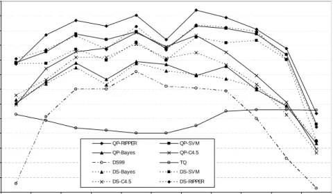
2.6 The averageF1-measure of the different techniques for varying specificity thresholdτes (τec=8). . . 33
2.7 The averageF1-measure of the different techniques for varying coverage thresholdτec (τes=0.4). . . 34
2.8 The averageF1-measure for hierarchies of different depths (τs =
τes=0.4,τc=τec=8). . . 35
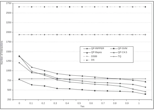
2.9 The average number of “interactions” with the databases as a function of thresholdτes(τec =8). . . 36
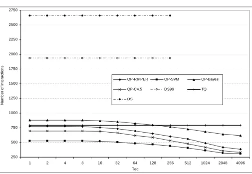
2.10 The average number of “interactions” with the databases as a function of thresholdτec(τes =0.4). . . 37
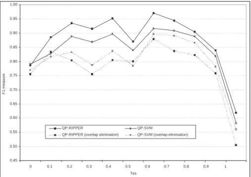
2.11 The averageF1-measure forQP-RIPPERandQP-SVMwith and without overlap elimination, as a function of thresholdτes(τec=
8). . . 38
2.12 The average F1-measure for the classification techniques over databases with boolean and vector-space interfaces, and for varyingτes(τec =8). . . 39
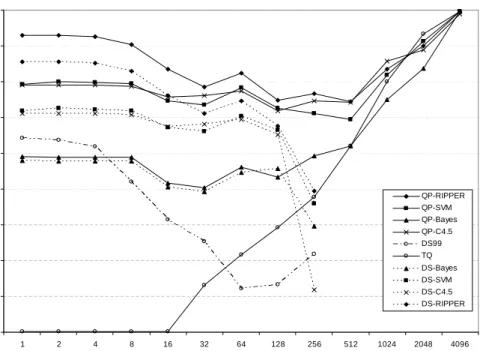
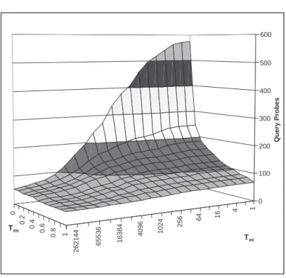
2.13 Average number of query probes for the Web databases as a function ofτesandτec. . . 42
3.1 Generalizing the classification algorithm from Figure2.4to gen-erate a content summary for a database using focused query probing. . . 55
3.2 Querying theCNN Sports Illustrateddatabase with focused probes. 56
3.3 Estimating unknowndf values. . . 57
3.4 A fraction of a classification hierarchy and content summary statistics for word “hypertension.” . . . 62
3.5 Using expectation maximization to determine the λi mixture
weights for the shrunk content summary of a databaseD. . . . 66
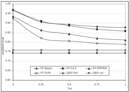
3.6a Weighted recallas a function of the specificity thresholdτes and
for theControlleddata set. . . 71
3.6c Spearman Rank Correlation Coefficientas a function of the speci-ficity thresholdτesand for theControlleddata set. . . 72
3.6d Relative error of thed f estimations, for words withd f >3, as a function of the specificity thresholdτesand for theControlled
data set. . . 72
3.6e Number of interactions per database, as a function of the speci-ficity thresholdτesand for theControlleddata set. . . 73
3.7a Weighted recallas a function of the specificity thresholdτes, for
theControlleddata set and for the case where theFP andQBS methods retrieve the same number of documents. . . 74
3.7b Unweighted recall as a function of the specificity thresholdτes,
for theControlled data set and for the case where theFP and QBSmethods retrieve the same number of documents. . . 74
3.7c Spearman Rank Correlation Coefficientas a function of the speci-ficity thresholdτes, for theControlleddata set and for the case
where the FP and QBS methods retrieve the same number of documents. . . 76
3.7d Number of interactions per database as a function of the speci-ficity thresholdτes, for theControlleddata set and for the case
where the FP and QBS methods retrieve the same number of documents. . . 76
3.8a Weighted recallfor pairs of database content summaries, for the Controlleddata set as a function of the number of common cat-egories in the database pairs. . . 78
3.8b Spearman Rank Correlation Coefficientfor pairs of database con-tent summaries, for theControlleddata set as a function of the number of common categories in the database pairs. . . 78
4.1 Associating content summaries with categories. . . 87
4.2 Selecting theKmost specific databases for a query hierarchically. 88
4.3 Exploiting a topic hierarchy for database selection. . . 89
4.4 Using shrinkage adaptively for database selection. . . 90
4.5 TheRkratio for CORI with stemming over theTREC4data set. 94
4.6 TheRk ratio for CORI without stemming over theTREC4data
set. . . 95
4.7 TheRkratio for CORI with stemming over theTREC6data set. 96
4.8 TheRk ratio for CORI without stemming over theTREC6data
set. . . 97
4.9 TheRkratio for bGlOSS with stemming over theTREC4data set. 98
4.10 The Rk ratio for bGlOSS without stemming over the TREC4
data set. . . 99
4.11 TheRkratio for bGlOSS with stemming over theTREC6data set.100
4.12 The Rk ratio for bGlOSS without stemming over the TREC6
data set. . . 101
4.13 TheRkratio for LM with stemming over theTREC4data set. . 102
4.14 TheRkratio for LM without stemming over theTREC4data set. 103
4.17 TheRkratio for CORI with stemming over theTREC4data set, with and without universal application of shrinkage. . . 109
4.18 TheRk ratio for CORI without stemming over theTREC4data
set, with and without universal application of shrinkage. . . 110
4.19 The Rk ratio for bGlOSS with stemming over theTREC4 data
set, with and without universal application of shrinkage. . . 111
4.20 The Rk ratio for bGlOSS without stemming over the TREC4 data set, with and without universal application of shrinkage. . 112
4.21 TheRkratio for CORI with stemming over theTREC4data set,
for summaries generated with (“-FreqEst” suffix) and without (“-NoFreqEst” suffix) the use of frequency estimation. . . 114
4.22 TheRk ratio for CORI without stemming over theTREC4data
set, for summaries generated with (“-FreqEst” suffix) and with-out (“-NoFreqEst” suffix) the use of frequency estimation. . . . 115
4.23 TheRkratio for CORI with stemming over theTREC6data set,
for summaries generated with (“-FreqEst” suffix) and without (“-NoFreqEst” suffix) the use of frequency estimation. . . 116
4.24 TheRk ratio for CORI without stemming over theTREC6data
set, for summaries generated with (“-FreqEst” suffix) and with-out (“-NoFreqEst” suffix) the use of frequency estimation. . . . 117
5.1 The recall of content summaryO(D,t)with respect to the “cur-rent” content summaryC(D), as a function of timetand aver-aged over each databaseDin the dataset. . . 126
5.2 The weighted recall of “old” QBS-based content summaries with respect to the “current” ones, as a function of the time T between updates and averaged over each database Din the dataset, for different scheduling policies (τ=0.5). . . 127
5.3 The weighted recall of “old”FPS-based content summaries with respect to the “current” ones, as a function of the time T be-tween updates and averaged over each databaseDin the dataset, for different scheduling policies (τ=0.5). . . 127
5.4 The unweighted recall of “old”QBS-based content summaries with respect to the “current” ones, as a function of the time T between updates and averaged over each database Din the dataset, for different scheduling policies (τ=0.5). . . 128
5.5 The unweighted recall of “old”FPS-based content summaries with respect to the “current” ones, as a function of the time T between updates and averaged over each database Din the dataset, for different scheduling policies (τ=0.5). . . 128
5.6 The precision of content summaryO(D,t)with respect to the “current” content summaryC(D), as a function of time t and
averaged over each databaseDin the dataset. . . 130
T between updates and averaged over each database Din the dataset, for different scheduling policies (τ=0.5). . . 131
5.8 The weighted precision of “old”FPS-based content summaries with respect to the “current” ones, as a function of the time T between updates and averaged over each database Din the dataset, for different scheduling policies (τ=0.5). . . 131
5.9 The unweighted precision of “old” QBS-based content sum-maries with respect to the “current” ones, as a function of the timeTbetween updates and averaged over each databaseDin the dataset, for different scheduling policies (τ=0.5). . . 132
5.10 The unweighted precision of “old”FPS-based content summaries with respect to the “current” ones, as a function of the timeT between updates and averaged over each database D in the dataset, for different scheduling policies (τ=0.5). . . 132
5.11 The KL divergence of content summaryO(D,t)with respect to the “current” content summaryC(D), as a function of time t and averaged over each databaseDin the dataset. . . 133
5.12 The KL divergence of “old”QBS-based content summaries with respect to the “current” ones, as a function of the time T be-tween updates and averaged over each databaseDin the dataset, for different scheduling policies (τ=0.5). . . 134
5.13 The KL divergence of “old”FPS-based content summaries with respect to the “current” ones, as a function of the time T be-tween updates and averaged over each databaseDin the dataset, for different scheduling policies (τ=0.5). . . 134
5.14 The survival functionS(t)for different domains (|D| = 1, 000,
τ=0.5,κ1=0.1,QBSsampling). . . 143 5.15 The precision of the updates performed by the different
schedul-ing algorithms, as a function of the average time between up-datesTand forτ=0.5, where theκ1feature is computed using
QBS-based summaries. . . 146
5.16 The precision of the updates performed by the different schedul-ing algorithms, as a function of the average time between up-dates T and τ = 0.5, where theκ1 feature is computed using
FPS-based summaries. . . 147
2.1 Real web databases in theWebset. . . 23
2.2 The F1-measure for QP-Bayes, with and without feature selec-tion (FS), and with and without confusion-matrix adjustment (CMA). . . 30
2.3 TheF1-measure forQP-C4.5, with and without confusion-matrix adjustment (CMA). . . 31
2.4 The F1-measure for QP-SVM, with and without feature selec-tion (FS), and with and without confusion-matrix adjustment (CMA). . . 31
2.5 TheF1-measure forQP-RIPPER, with and without feature selec-tion (FS), and with and without confusion-matrix adjustment (CMA). . . 32
2.6 Results of three-fold cross-validation over theWebdatabases. . 40
2.7 The performance of crawling- and query-based classification for five databases (τes =0.4,τec =8). . . 44
2.8 The crawling-based classification and associated precision (P) and recall (R) for five databases after crawling different frac-tions of each database (τes=0.4,τec=8). . . 45
3.1 A fragment of the content summaries of two databases. . . 51
3.2 The category mixture weights for two databases. . . 65
3.3 Some of the real web databases in theWebdata set. . . 67
3.4 Weighted recall, Spearman Rank Correlation Coefficient, and num-ber of interactions per database, for theWeb,TREC4, andTREC6 data sets and for the case where FP-SVM and QBS-SVM re-trieve the same number of documents. . . 77
3.5a Weighted recall for pairs of database content summaries, as a function of the number of common categories in the database pairs and for theWeb,TREC4, andTREC6data sets. . . 79
3.5b Spearman Rank Correlation Coefficientfor pairs of database con-tent summaries, as a function of the number of common cate-gories in the database pairs and for theWeb,TREC4, andTREC6 data sets. . . 80
3.6a Weighted recallwr. . . 81
3.6b Unweighted recallur. . . 81
3.7a Weighted precisionwp. . . 82
3.7b Unweighted precisionup. . . 82
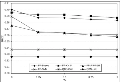
3.8 Spearman Correlation CoefficientSRCC. . . 83
4.1 Percentage of query-database pairs for which shrinkage was applied. . . 108
5.1 Distribution of domains in our dataset. . . 125
5.2 The coefficients of the Cox model, when trained for various sets of features and for different sampling methods for computing theκ1feature. . . 140 5.3 The parameters for the baseline survival functions for the five
domains. The baseline survival functions describe the survival time of a databaseDin each domain with size|D|=1 (ln(|D|) = 0), with average distance between the sample summariesκ1=0 (computed usingQBSorFPS) and for thresholdτ=0. . . 141
5.4 Optimal content-summary update frequencies for two databases.144
First and foremost, I would like to thank my advisor, Luis Gravano, for his truly exceptional guidance and help. He helped me inmanyaspects of my aca-demic and personal life and vindicated multiple times my decision to come to Columbia for my PhD studies. I am indebted to him for everything. Much of the work in this thesis is a result of collaboration. Mehran Sahami gave me invaluable advice and helped me understand in depth many machine learning algorithms. The work in Chapter2is joint work with him and Luis. I have also benefited from my collaboration with Junghoo Cho and Alexandros Ntoulas. The work in Chapter5is the result of the collaboration with Junghoo, Alexandros, and Luis. Many thanks also go to Jamie Callan, who served on my thesis committee, gave me great comments, and helped me improve the clarity and precision of the final manuscript.
I also wish to thank all the past and present members of the Columbia Data-base Group for countless discussions and useful feedback. In particular, Ken Ross helped me improve my presentation skills and was a source of useful criticism for my work. Eugene Agichtein, Nicolas Bruno, and Am´elie Mar-ian were always available for discussion (not necessarily about research) and always ready to share stories about Luis’ comments on our write-ups. I would also like to thank the members of the SDARTS team: Jiangcheng Bao, Tom Barry, Alexander Besidski, Yan Besidski, Noah Green, Boyle Lee, and Sergey Sigelman. They have helped me tremendously with the implementa-tion and they turned my research prototypes into a usable product.
My friends (that I will not list here) helped me achieve balance in my life. Their help was invaluable and I know that without them I would have never finished this thesis.
Κλείνοντας, θα ήθελα να ευχαριστήσω τους γονείς μου, για όλα όσα έκαναν για μένα. Χωρίς αυτούς, και χωρίς την αμέριστη συμπαράστασή τους, δεν θα είχα καταφέρει τίποτα. Ξέρω ότι ποτέ δε θα μπορέσω να τους το ανταποδώσω. Μητέρα, μακάρι να έχω τη δύναμη, την υπομονή και το χαμόγελό σου. Πατέρα, ξέρω πόσο περήφανος ήσουν πάντοτε για μένα. Αυτή τη στιγμή μόνο ένα πράγμα μπορώ να σου υποσχεθώ: ῾῾Πάντα έτσι...᾿᾿. ix
Chapter
1
Introduction
The World-Wide Web continues to grow. Unprecedented amounts of infor-mation are available on regular web pages and also in valuabletext databases whose contents are exposed via search interfaces. Web search engines such as Google1 provide effective access to web pages but, unfortunately, text da-tabases are sometimes more challenging to handle. Specifically, text data-bases often have their contents “hidden” behind search interfaces and their documents cannot be accessed directly through hyperlinks, which effectively makes the database contents invisible to traditional search engines. We refer to such databases as hidden-web text databases. Examples of hidden-web text databases include the Library of Congress database, the US Patent and Trade-mark database, the PubMed database, newspaper archives, and many other valuable sources of information. The main purpose of this thesis is to devise accurate and efficient techniques for classifying and searching hidden-web text databases, thus providing critical building blocks to enable web users to browse and search these databases as easily and efficiently as users access regular web pages via web search engines.
To support browsing, it is desirable to organize text databases in a classifica-tion scheme, so that users can navigate through categories to locate databases of interest. In the past, there have been efforts to manually classify text da-tabases into Yahoo!-like hierarchical categorization schemes. Unfortunately, manual approaches do not scale well over the web, so we present an auto-matic method to place databases in a classification scheme in an accurate and efficient manner.
To support searching, we can buildmetasearchers, which provide a uniform interface for querying multiple databases at once. A typical metasearcher may provide access to hundreds or thousands of databases. However, only a few of the available databases may contain relevant documents for a given query. Therefore, for efficiency and accuracy it is important not to broadcast
the query to all available databases but rather query only databases with rel-evant content. The database selection component of a metasearcher typically relies on a statistical summary of the database contents, which should be com-pleteand reflect the actual,currentcontents of the databases. We present key technologies both for generating accurate and up-to-date database summaries and for improving existing database selection algorithms.
Specifically, the key contributions of this thesis are as follows:
• In Chapter2, we presentQProber, a classification algorithm for text data-bases. QProbercategorizes databaseswithout retrieving any document. In-stead,QProberuses just the number of matches generated from a small number of topically focused query probes. For example, a database that generates a large number of matches for queries like [cancer] and [heart disease] but not for [algorithm] and [operating systems] is more likely to be about “Health” than about “Computers.” The query probes are automatically generated using state-of-the-art supervised machine learn-ing techniques and are typically short. We present experimental results showing that QProberproduces highly accurate classification decisions, sending only a small number of queries to each database.
• In Chapter 3, we build on the classification technique from Chapter 2
and present an algorithm to derive content summaries from hidden-web text databases by using “focused query probes.” The probes adaptively extract documents that are representative of the topic coverage of the databases. We also present a technique for estimating the absolute doc-ument frequency of the database words, which is important for database selection. Unfortunately, Zipf’s law virtually guarantees that any con-tent summary constructed from a reasonably small document sample will suffer from data sparseness and will not contain many words that appear in the database. To address this problem, we exploit the hierar-chical categorization of the databases and adapt the notion of “shrink-age” —a form of smoothing that has been used successfully for doc-ument classification— to the content summary construction task. Our evaluation suggests that the generated content summaries are signifi-cantly more complete than their “unshrunk” counterparts.
• In Chapter4, we present two database selection algorithms that exploit database classification to improve the quality of search results in the face of incomplete, sample-based content summaries. Both algorithms are based on the observation that topically similar databases tend to have related content summaries. First, we present a hierarchical selec-tion algorithm that directs queries to the most promising categories and then to the best databases in these categories. Then, we present a “flat” selection strategy that exploits the database categorization implicitly, via the shrinkage-based content summaries. Our algorithm adaptively de-cides whether to use the shrinkage-based content summaries or their unshrunk counterparts. Our experimental evaluation shows that, in
the presence of incomplete content summaries, the proposed algorithms outperform the state-of-the-art database selection techniques.
• In Chapter 5, we present a study on the evolution of web databases. Content summaries of static databases do not change over time. How-ever, databases are rarely static and the statistical summaries that de-scribe their contents need to be updated periodically to reflect content changes. To understand how real-world databases change over time and how these changes propagate to the database content summaries, we start by studying how the content summaries of152real web data-bases changed every week, over one year. Then, we use “survival anal-ysis” techniques to examine which parameters can help predict when the content summaries need to be updated. Based on the conclusions of this study, we develop algorithms that analyze various characteristics of the databases and their update history to predict when the content sum-maries need to be modified, thus avoiding overloading the databases unnecessarily.
Finally, in Chapter6we discuss related work, while in Chapter7we present conclusions and directions for future research.
Chapter
2
Classifying Hidden-Web Text
Databases
The World-Wide Web continues to grow and unprecedented amounts of infor-mation are available on regular web pages that search engines such as Google crawland index. In addition, the web also hosts valuabletext databaseswhose contents are exposed via search interfaces. The general problem of accurate information access and retrieval on the web thus continues to escalate. A particular aspect of this problem, on which we focus in this chapter, is the categorization of text databases according to their topic.
The information stored in text databases is often of high quality, as the follow-ing example illustrates:
Example1 Consider the US Patent and Trademark (USPTO) database, which con-tains the full text of all the patents awarded in the US since 19761. If we query USPTO for patents with the keywords wireless AND network, USPTO returns 28,013 matches (as of May 27th,2004), corresponding to distinct patents that con-tain these keywords. The full text of the patents is stored locally at the USPTO site and is not distributed over the web.
Unfortunately, text databases often have their contents “hidden” behind search interfaces and their documents cannot be accessed directly through hyper-links. We refer to such databases as hidden-web text databases. For our pur-poses, a hidden-web text database is a collection of text documents that is searchable through a web-accessible search interface. The documents in a text database do not necessarily reside on a single centralized site, but can be scattered over several sites. Traditional search engines cannot index such text databases, since search engines rely on hyperlinks to reach the documents that they index. Hence, search engines ignore the contents of hidden-web databases, as the following real example shows:
Example1 (cont.) Unfortunately, the high-quality contents of the USPTO data-base are not crawlable by traditional search engines. A query2on Google that finds
the pages in the USPTO database with the keywords “wireless” and “network” re-turns0matches (as of May 27th,2004), which illustrates that the valuable content available through this database is ignored by traditional search engines.
Additionally, some web sites prevent crawling by restricting access via a robots.txtfile. Such sites then also become de-facto non-crawlable.
This chapter focuses on the classification of hidden-web text databases. In order to effectively guide users to the appropriate databases, some web sites (described in more detail below) have undertaken the arduous task of manu-ally classifying these databases into a Yahoo!-like hierarchical categorization scheme. While we believe this type of categorization to be immensely helpful to web users trying to find information relevant to a given topic, it is ham-pered by the lack of scalability inherent in manual classification. By providing efficient and automatic means for the accurate classification of text databases into topic hierarchies, we hope to alleviate the scalability problems of manual database classification, and make it easier for end-users to find the relevant information they are seeking on the web.
Consequently, in this chapter we describe our system, namedQProber, which automatically categorizes hidden-web text databasesinto topic hierarchies. QProber uses a combination of machine learning and database querying techniques. We use machine learning techniques to initially build document classifiers. Rather than actually using these classifiers to categorize individual docu-ments, we extract classification rules from the document classifiers, and we transform these rules into a set of query probes that can be sent to the search interface of the available text databases. Our algorithm then simply uses the number of matches reported for each query to make classification decisions, without having to retrieve and analyze any of the actual database documents. This makes our approach very efficient and scalable.
The contributions presented in this chapter are organized as follows. In Sec-tion2.1, we more formally define and provide various strategies for text da-tabase classification. In Section2.2, we present the details of our query prob-ing algorithm for database classification and describe an algorithm to extract query probes from a variety of both rule-based and linear document classi-fiers. In Sections2.3and2.4, we provide the experimental setting and results, respectively. We compare variations ofQProberwith existing methods for au-tomatic database classification.QProberis shown to be both more accurate as well as more efficient on the database classification task. Also, we examine how different parameters affect the performance ofQProberand report results for different classifier types as well as for a variety of probing strategies and document retrieval models. In Section2.5, we show howQProber can be at-tractive for classifyingcrawlabletext databases as well, as an alternative to a more expensive crawling-based classification strategy. Finally, in Section2.6,
WNBA CBS Sportsline
- Basket
ESPN Baseball Basketball Volleyball
Arts Computers Health Science Sports
Root ... ... ... ... ... ... ... ... ... ...
Figure2.1:Portion of the InvisibleWeb classification scheme.
we provide further discussion, and in Section 2.7 we conclude the chapter. The bulk of this chapter has appeared in [IGS00,IGS01b,GIS02,GIS03].
2
.
1
Classification of Text Databases
In this section, we discuss how we can organize hidden-web text databases in a hierarchical categorization scheme, which users can browse to find the resources of interest. First, in Section2.1.1, we define the hierarchical classi-fication schemes that we will consider. Then, in Section2.1.2, we define our text database classification task over a categorization scheme of choice.
2
.
1
.
1
Hierarchical Classification Schemes
Web directories like Yahoo! organize web pages into categories for users to browse. In this section, we extend this notion to hidden-web text databases. Several commercial web directories have started tomanuallyclassify hidden-web text databases, so that users can browse through these categories to find the databases of interest. Examples of such directories include InvisibleWeb3 and SearchEngineGuide4. Figure2.1shows a small fraction of InvisibleWeb’s classification scheme.
Formally, we can define a hierarchical classification scheme like the one used by InvisibleWeb as follows:
Definition1 Ahierarchical classification schemeis a rooted directed tree whose
nodes correspond to (topic) categories and whose edges denote specialization. An edge from category v to another category v0 indicates that v0 is a subcategory of v.
3http://www.invisibleweb.com
Given a classification scheme, our goal is to automatically populate it with text databases, where we assign each database to the “best” category or cat-egories in the scheme. For example, InvisibleWeb has manually assigned WNBA to the“Basketball”category in its classification scheme. In general we can define what category or categories are “best” for a given database in sev-eral different ways, according to the needs that the classification will serve. We describe different such approaches next.
2
.
1
.
2
The Text Database Classification Task
We now turn to the central issue of how to automatically assign databases to categories in a classification scheme, assuming complete knowledge of the contents of these databases. Of course, in practice we will not have such com-plete knowledge, so we will have to use the probing techniques of Section2.2
to approximate the “ideal” classification definitions that we give next. To assign a text database to a category or set of categories in a classification scheme, one possibility is to manually inspect the contents of the database and make a decision based on the results of this inspection. Incidentally, this is the way in which commercial web directories like InvisibleWeb operate. This approach might produce good quality category assignments but, of course, is expensive (it includes human participation) and does not scale well to large numbers of databases.
Alternatively, we could follow a less manual approach and determine the cate-gory of a text database based on the catecate-gory of thedocumentsthat it contains. We can formalize this approach as follows. Consider a web databaseDandn categoriesC1, . . . ,Cn. If we knew the category of each of the documents inside
D, then we could use this information to classify database Din at least two different ways. A coverage-basedclassification will assign Dto all categories for which Dhas sufficiently many documents. In contrast, aspecificity-based classification will assignDto the categories that cover a significant fraction of D’s holdings.
Example2 Consider topic category “Basketball.” CBS SportsLine has a large number of articles about basketball and covers not only women’s basketball but other basketball leagues as well. It also covers other sports like football, baseball, and hockey. On the other hand,WNBAonly has articles about women’s basketball. The way that we will classify these sites depends on the use of our classification. Users who prefer to seeonlyarticles relevant to basketball might prefer aspecificity-basedclassification and would like to have the siteWNBAclassified into node“Basketball.” However, these users would not want to have CBS SportsLine in this node, since this site has a large number of articles irrelevant to basketball. In contrast, other users might prefer to have only databases with a broad and comprehensive coverage of basketball in the“Basketball”node. Such users might prefer acoverage-basedclassification and would like to findCBS SportsLinein the“Basketball”node, which has a large
number of articles about basketball, but notWNBAwith only a small fraction of the total number of basketball documents.
More formally, we can use the number of documents in each category that we find in databaseDto define the following two metrics, which we will use to specify the “ideal” classification ofD. Later, in Section2.2.2, we show how we can approximate these metrics.
Definition2 Consider a database D, a hierarchical classification scheme C, and a category Ci ∈ C. The coverage of a databaseD for Ci, Coverage(D,Ci), is the
number of documents in D in category Ci:
Coverage(D,Ci) =number of D documents in category Ci
Coverage(D,Ci) defines the “absolute” amount of information that database
Dcontains about categoryCi.5
Definition3 In the same setting as Definition2, thespecificity of a database D for Ci, Specificity(D,Ci), is the fraction of documents in category Ci in D. More
formally, we have:
Specificity(D,Ci) =
Coverage(D,Ci)
|D|
where|D|is the number of documents in the database.
Specificity(D,Ci) gives a measure of how “focused” the database D is on a
categoryCi. The value ofSpecificity ranges between 0and 1. For notational
convenience, we define:
Coverage(D) = hCoverage(D,Ci1), . . . ,Coverage(D,Cim)i Specificity(D) = hSpecificity(D,Ci1), . . . ,Specificity(D,Cim)i when the set of categories{Ci1, . . . ,Cim}is clear from the context.
Now, we can use theSpecificityandCoveragevalues to decide how to classify D into one or more categories in the classification scheme. As described above, aspecificity-based classificationwould classify a database into a category when a significant fraction of the documents it contains are of this specific category. Alternatively, acoverage-based classificationwould classify a database into a category when the database has a substantial number of documents in 5It would be possible to normalizeCoveragevalues to be between0and1by dividing by the
total number of documents in categoryCiacrossalldatabases.Coveragewould then measure the
fraction of the universally available information aboutCithat is stored inD. Alternatively, we
could defineCoveragein terms of a variant of the inverse-document-frequency metric (idf) [SM83] to express the extent to which a database covers a topic that is rare overall. Although intuitively appealing, such definitions would be “unstable” since each creation, deletion, or modification of a web database would change theCoverageof the other available databases.
the given category. In general, however, we are interested in balancing both SpecificityandCoveragethrough the introduction of two associated thresholds,
τs andτc, respectively, as captured in the following definition.
Definition4 Consider a classification scheme C with categories C1, . . . ,Cn, and a
database D. TheIdeal classification of DinC is the setIdeal(D)of categories Ci
that satisfy the following conditions: • Specificity(D,Ci)≥τs
• Coverage(D,Ci)≥τc
• Coverage(D,Ck)<τcor Specificity(D,Ck)<τs for each of the children Ckof
Ci
where0≤τs ≤1andτc≥1are given thresholds.
TheIdealclassification definition given above provides alternative approaches for “populating” a hierarchical classification scheme with text databases, de-pending on the values of the thresholds τs and τc. These values should
ul-timately be determined according to the intended use and audience of the classification scheme.6
For example, as an “editorial decision,” we might decide that only databases with a majority of documents on a particular category should be classified under that category. In this case, the specificity thresholdτs should be set to
0.5. The Borland database of technical, programming-related articles7, with
about60% of its articles about theJavaprogramming language, would then be classified under theJavacategory. In contrast, if we decide to be somewhat more “flexible,” we might insist that, say 30% of the database articles be on a particular category. The Borland database, with about30% of its contents aboutC/C++would then be classified under theC/C++ category in addition to theJavacategory. A similar analysis applies to the editorial choice of the value of the coverage thresholdτc.
As an alternative to defining the values of the τs andτcthresholds explicitly,
we could establish these values “by example.” Specifically, we could provide a few examples of known databases together with their “correct” classification. We could then derive the choice of τs and τc that best fit the classification
examples. While we do not explore this direction further, we should note that we follow a closely related idea for the experiments in Section 2.4.3, where 6The choice of thresholds might also depend on other factors. For example, consider a
hy-pothetical database with a “perfect” retrieval engine. Coverage might then be more important than specificity for this database if users extract information from the database by searching. The retrieval engine identifies exactly the on-topic documents for a query, making the presence of off-topic documents in the database irrelevant. Then, the “perceived specificity” of the database for a given category for which it has sufficientCoverageis1, which would argue for the use of a coverage-based classification of the database.
we attempt to estimate the τs andτcused “implicitly” by the human experts
in at the InvisibleWeb site.
Next, we introduce a technique for automatically populating a classification scheme according to the ideal classification of choice.
2
.
2
Classifying Databases through Probing
In the previous section, we defined how to classify a database based on the number of documents that it contains in each topic category. Unfortunately, databases typically do not export such category-frequency information. In this section, we describe how we can approximate this information for a given database without accessing its contents. The whole procedure is divided into two parts. First, we train our system for a given classification scheme. Then, we probe each database with queries to decide the categories to which it should be assigned. More specifically, we follow the algorithm below:
1. Train a document classifier with a set of preclassified documents (Sec-tion2.2.1).
2. Extract a set of classificationrulesfrom the document classifier and trans-form classifier rules into queries (Sections2.2.2and2.2.3).
3. Adaptively issue queries to databases, extracting and adjusting the num-ber of matches for each query using the classifier’s “confusion matrix” (Section2.2.4).
4. Classify databases using the adjusted number of query matches (Sec-tion2.2.5).
2
.
2
.
1
Training a Document Classifier
Our database classification technique relies on a document classifier to create the probing queries, so our first step is to train such a classifier. We use super-vised learning to construct the classifier from a set of preclassified documents. The procedure follows a sequence of steps, described below.
The first step, which helps both efficiency and effectiveness, is to eliminate from the training set all words that appear either very frequently or very in-frequently in the training documents. This initial “feature selection” step is based on Zipf’s law [Zip49], which provides a functional form for the distri-bution of word frequencies in document collections. Very frequent words are usually auxiliary words that bear no information content (e.g., “am,” “and,” “so” in English). Infrequently occurring words are not very helpful for clas-sification either, because they appear in so few documents that there are no significant accuracy gains from including such terms in a classifier.
The elimination of words dictated by Zipf’s law is a form of feature selection. However, frequency information alone is not, after some point, a good indica-tor to drive the feature selection process further. Thus, we use an information theoretic feature selection algorithm that eliminates the terms that have the least impact on the class distribution of documents [KS97,KS96]. This step eliminates the features that either do not have enough discriminating power (i.e., words that are not strongly associated with one specific category) or fea-tures that are redundant given the presence of another feature. Using this algorithm we decrease the number of features in a principled way and we can use a much smaller subset of words to create the classifier, with minimal loss in accuracy. The surviving features are generally useful for classification purposes, so classifiers constructed from these features tend to generalize well to unseen data [KS97,KS96]. In Section2.4.1, we evaluate experimentally the effect of feature selection on database classification.
After selecting the features (i.e., words) that we will use for building the docu-ment classifier, we can use an existing machine learning algorithm to create a document classifier. Many different algorithms for creating document classi-fiers have been developed over the last few decades. Well known techniques include the Naive Bayes classifier [DHS00], C4.5 [Qui92], RIPPER [Coh96], and Support Vector Machines [Vap98], to name just a few. These document classifiers work with a flat set of categories. To define a document classifier over an entire hierarchical classification scheme (Definition1), we train one flat document classifier for eachinternalnode of the hierarchy.
Once we have trained a document classifier, we could use it to classify all the documents in a database of interest to determine the number of documents about each category in the database. Of course, this requires having access to the whole contents of the database, which is not a realistic requirement for hidden-web databases. We relax this requirement presently.
2
.
2
.
2
Defining Query Probes from a Rule-Based Document
Classifier
In this section, we first describe the class ofrule-based classifiersand then we show how we can use a rule-based classifier to generate a set ofquery probes that will help us estimate the number of documents for each category of interest in a text database.
In arule-based classifier, the classification decisions are based on a set of logical rules: the antecedents of the rules are conjunctions of words and the conse-quents are the category assignments for documents. For example, the follow-ing rules are part of a classifier for the three categories“Sports,” “Health,”and “Computers”:
ibm AND computer→Computers
diabetes→Health
cancer AND lung→Health
intel→Computers
Such rules are used to classify previously unseen documents (i.e., documents not in the training set). For example, the first rule would classify all docu-ments containing the words “ibm” and “computer” into the category “Com-puters.”
Definition5 Arule-based document classifierfor aflatcategory set C={C1, . . . ,Cn}
consists of a set of rules pk →Clk,k=1, . . . ,m, where pkis a conjunction of words and Clk ∈ C. A document d matches a rule pk → Clk if all the words in that rule’s antecedent, pk, appear in d. If a document matches multiple rules with dif-ferent classification decisions, the final classification decision depends on the specific implementation of the rule-based classifier.
We can simulate the behavior of a rule-based classifier over all documents of a database by mapping each rule pk → Clk of the classifier into a boolean queryqkthat is the conjunction of all words inpk. Thus, if we send the query
probeqkto the search interface of a databaseD, the query will match exactly the f(qk)documents in the databaseDthat would have been classified by the associated rule into category Clk. For example, we map the rulejordan AND bulls →Sports into the boolean query [jordan AND bulls]8. We expect this
query to retrieve mostly documents in the “Sports” category. Now, instead of retrieving the documents themselves, we just keep the number of matches reported for this query (it is quite common for a database to start the results page with a line like “Xdocuments found”; even ballpark approximations are good enough for our classification task), and use this number as a measure of how many documents in the database match the condition of this rule. From the number of matches for each query probe, we can construct a good approximation of the Coverageand Specificity vectors for a database D (Sec-tion2.1). We can approximate the number of documents in Din categoryCi
as the total number of matches from all query probes derived from rules with categoryCias a consequent. Using this information we can approximate the
CoverageandSpecificityvectors forDas follows:
Definition6 Consider a text database D and a rule-based classifier for a set of cat-egories C. For each query probe q derived from the classifier, database D returns the number of matches f(q). The estimated coverage of D for a categoryCi ∈ C,
ECoverage(D,Ci), is the total number of matches for the Ci query probes.
ECoverage(D,Ci) =
∑
q is a query probe for Cif(q)
Definition7 In the same setting as Definition6, theestimated specificity of D forCi, ESpecificity(D,Ci), is
ESpecificity(D,Ci) =
ESpecificity(D,Parent(Ci))·ECoverage(D,Ci)
∑Cjis a child of Parent(Ci)ECoverage(D,Cj)
As a special case, ESpecificity(D, “root”) =1.
Thus, Definition 7 tells us that the estimated specificity for a category Ci
in D is the estimated percentage of documents in D that are in Parent(Ci) multiplied by the percentage of documents inParent(Ci)that are also inCi.
For notational convenience, we define:
ECoverage(D) = hECoverage(D,Ci1), . . . ,ECoverage(D,Cim)i ESpecificity(D) = hESpecificity(D,Ci1), . . . ,ESpecificity(D,Cim)i when the set of categories{Ci1, . . . ,Cim}is clear from the context.
Example3 Consider a small, rule-based document classifier for categories C1=“Sports,”
C2=“Computers,” and C3=“Health” consisting of the five rules listed previously. To
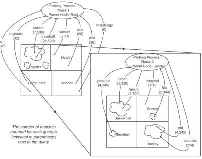
classify the ACM Digital Library database, we send the query [ibm AND computer], which results in 6646matching documents (Figure2.2). The other four queries re-turn the matches described in Figure2.2. Using these numbers we can estimate that the ACM Digital Library has0documents about“Sports,”6646+2380=9026 docu-ments about“Computers,” and18+34=52documents about“Health”. Thus, the ECoverage(ACM) vector for this set of categories is:
ECoverage(ACM) = (0, 9026, 52) and the respective ESpecificity(ACM) vector is:
ESpecificity(ACM) = µ 0 0+9026+52, 9026 0+9026+52, 52 0+9026+52 
As defined above, the computation ofECoveragemight count documents more than once, since the same document might match multiple query probes. To address this issue, we could issue query probes in order, augmenting each query probe with the negation of all earlier query probes. Consider the five example rules above, in the order they are listed. The first query would be [ibm AND computer], as before. However, the second query becomes [jordan AND bulls AND NOT (ibm AND computer)], to not match (and count) any doc-ument that matches the first query probe. This technique ensures that the final number of matches for each category is not artificially inflated by docu-ments that match multiple query probes. Unfortunately, if implemented in a naive way, this overlap-elimination strategy may result in rather long query
ACM Digital Library 34 matches 6646 matches 0 matches 18 matches 2380 matches diabetes intel cancer AND lung jordan AND bulls ibm AND computer
Figure2.2: Sending probes to the ACM Digital Library database with queries derived from a document classifier.
probes, which might not be accepted by the databases. This problem could be partially solved by “breaking” the long queries into smaller conjunctive queries. Then, by exploiting the inclusion-exclusion principle and the num-ber of matches for each of the smaller probes, we can calculate the numnum-ber of matches for the complex query. For example, instead of sending the query [jordan AND bulls AND NOT (ibm AND computer)], we can find the number of matches for the query [jordan AND bulls] and then subtract from it the number of matches generated for the query [jordan AND bulls AND ibm AND computer]. Unfortunately, the number of probes needed for this strategy in-creases exponentially with the query length. In Section2.4, we experimentally evaluate the benefits of this expensive overlap-elimination strategy.
2
.
2
.
3
Extracting Query Probes from Numerically
Parameter-ized Document Classifiers
We have seen so far that we can directly use a rule-based classifier to generate the query probes required for our database classification technique. However, restricting QProber to only rule-based classifiers would prevent us from ex-ploiting other classification strategies as they are developed. In this section, we describe how we can adapt numerically parameterized classifiers for use withQProber. In particular, we describe an algorithm that approximates a lin-ear binary classifier with a set of classification rules. We also describe briefly how the same algorithm can be modified to approximate different types of classifiers. Finally, we give some pointers to existing work in the area of rule extraction. Before describing the algorithm in detail, we define the terminol-ogy that we will use.
Definition8 Abinary classifierdecides whether a document, represented using m features (i.e., words in our context), belongs to one class or not. A binary linear
classifiermakes this decision by calculating, during the training phase, m weights w1, . . . ,wm and a threshold b determining a hyperplane such that all points t =
ht1, . . . ,tmiin the hyperplane satisfy the equation: m
∑
i=1
witi=b (2.1)
This hyperplane divides the m-dimensional document space into two regions: the region with the documents that belong to the class in question, and the region with all other documents. Then, given the m-dimensional representationhs1, . . . ,smiof a
document [SB88], the classifier calculates the document’s “score” as∑mi=1wisi. The
value of this score relative to that of threshold b determines the classification decision for the document.
A large number of classifiers fall into the category of linear classifiers. Ex-amples include Naive Bayes and Support Vector Machines (SVM) with linear kernel functions. Details on how to calculate these weights for SVMs and for Naive Bayesian classifiers can be found in [Bur98] and in [Nil90], respectively. A classifier fornclasses can be created usingnbinary classifiers, one for each class. Note that such a composite classifier may result in a document being categorized into multiple classes or into no classes at all.
We can use Equation 2.1 to approximate a linear classifier with a rule-based classifier that will be used to generate the query probes. The intuition behind the rule-extraction algorithm that we introduce next is that the presence of a few highly weighted terms in a document suffices for the linear classifier to make a positive decision (i.e., go above threshold). Our rule-extraction algo-rithm works by generating rules iteratively. In each iteration we create rules of different length, i.e., with a different number of terms in the antecedents. During the first iteration, we consider only rules with one term. If the weight of a term is higher than the thresholdb, then this term is qualified to form a rule, since the presence of this term alone suffices to classify a document into the category. For efficiency and simplicity, the rules are formed as conjunc-tions of terms with no negaconjunc-tions. After creating all the rules with one term, the algorithm proceeds to the next iteration, in which it creates rules with two terms, and so on.
The algorithm is described in more detail in Figure2.3. In general, when all weights defining the separating hyperplane are non-negative, a sufficient condition for a set of terms to form a rule is that the sum of the weights of its terms exceeds the value of the threshold b. While the classifiers that we consider do not necessarily produce exclusively non-negative weights, we nevertheless have found that our sufficiency criteria for extracting rules works well. Our algorithm can be further optimized if we impose more constraints on the rule-generation process (e.g., by bounding the number of generated rules or the number of words in each rule), but such optimizations are beyond the scope of this thesis.
GenerateRules(int[]w, intb)
RulesR=∅
CandidatesC={{f1},{f2}, . . . ,{fm}}
for eachsets∈C
support = CalculateSupport(s,w)
ifsupport<e
thenC=C−s
k=1
while(C6=∅)
for eachsets∈C
support = CalculateSupport(s,w) r= GetRule(s)
ifsupport>band Useful(r)
thenR=R∪r;C=C−s C= GenerateNewSets(C,k) k=k+1 returnR CalculateSupport(sets, int[]w) intsup=0
for eachtermti∈s
sup=sup+wi
returnsup
GenerateNewSets(setC, intk)
// All sets inChavekterms setR=∅
for eachsetci∈C
find the setFof all sets inC that havek−1 terms in common withci
for eachsetfi∈F
R=R∪ {ci∪fi}
returnR
Figure2.3:Generating rules from a set of weightswiand a thresholdb.
As an additional property, the rules that we derive from a classifier have to be “useful”: a rule is useful if and only if it covers “sufficiently many” examples from the training set and its precision is greater than0.5(i.e., it matches more correct documents than incorrect ones). The terms that form an extracted rule are removed from further consideration and will not participate in later iter-ations of the algorithm. Also, training examples that match a produced rule are removed from the training set, and will not be used in later iterations. To proceed to the next iteration, the algorithm expands unused term sets by one term, in a spirit similar to an algorithm for finding “association rules” [AS94]. In our algorithm, the “support” of a set of terms is defined as the sum of the weights of its terms, and the objective is to extend the “small” itemsets (i.e., the sets of terms whose sum of weights is smaller thanb) to get new itemsets with larger support.
Our rule extraction algorithm can be used for classifiers that divide the space using a non-linear polynomial as well. For example, SVMs with polynomial kernels can be treated in a similar way by considering the weights associated with all the higher order terms in the function.
The task of rule extraction from classification models that do not explicitly represent their output as rules has been studied extensively in the machine learning community. An example is the C4.5RULES algorithm [Qui92], which generates a set of production rules from a decision tree. Another example is Trepan[Cra96], which extracts a comprehensible set of rules from a neural network. Flake et al. [FGLG02] describe an algorithm for extraction of rules from nonlinear SVMs. The ongoing research in rule extraction can be directly leveraged to adapt different learning models for use withQProber.
2
.
2
.
4
Adjusting Probing Results
QProber relies on document classifiers to define query probes and obtain category-frequency information for a database. Unfortunately, document clas-sifiers are not perfect, because they can misclassify documents into incorrect categories and leave any documents that do not match any rules unclassified. In this section, we present a novel algorithm to adjust our initial probing results to account for such potential errors.
It is common practice in the machine learning community to report document classification results using aconfusion matrix[KP98]. We adapt this notion of a confusion matrix for use in our probing scenario:
Definition9 The normalized confusion matrix M = (mij) of a set of query
probes for categories C1, . . . ,Cn is an n×n matrix, where mij is the sum of the
number of matches generated from documents in category Cj for category Ci query
probes, divided by the total number of documents in category Cj.
In a perfect setting, the probes for Ci match onlydocuments inCi and each
document in Ci matchesexactly one probe forCi. In this case the confusion
matrix is the identity matrix.
The algorithm to create the normalized confusion matrixMis:
1. Generate the query probes from the classifier rules and probe a database of unseen, preclassified documents (i.e., the development set).
2. Create an auxiliary confusion matrix X = (xij)and setxij equal to the
sum of the number of matches fromCjdocuments for categoryCiquery
probes.
3. Normalize the columns of X by dividing column j with the number of documents in the development set in category Cj. The result is the
normalized confusion matrix M.
Example4 Suppose that we have a document classifier for three categories C1=“Sports,”
C2=“Computers,” and C3=“Health.” Consider 5100 unseen, pre-classified
docu-ments with1000 documents about “Sports,” 2500documents about “Computers,” and 1600documents about “Health.” After probing this set with the query probes generated from the classifier, we construct the following confusion matrix:
M= 600 1000 2500100 1600200 100 1000 20002500 1600150 50 1000 2500200 10001600 = 0.60 0.04 0.125 0.10 0.80 0.09375 0.05 0.08 0.625
Element m23 = 1600150 indicates that the probes for C2 mistakenly generated 150
matches from the documents in C3 and that there are a total of 1600 documents
Interestingly, multiplying the confusion matrix with theCoveragevector rep-resenting the correct number of documents for each category in the devel-opment set yields, by definition, the ECoverage vector with the number of documents in each category in the development set as matched by the query probes.
Example5 The Coverage vector with the actual number of documents in the develop-ment set T for each category is Coverage(T) = (1000, 2500, 1600). By multiplying M by this vector, we get the distribution of document categories in T as estimated by the query probing results.
0.60 0.040.10 0.80 0.093750.125 0.05 0.08 0.625 | {z } M × 10002500 1600 | {z } Coverage(T) = 2250900 1250 | {z } ECoverage(T)
Proposition1: The normalized confusion matrix M is invertible when the rules of the document classifier used to generate M match more correct documents than incorrect ones.2
Proof1: From the assumption on the document classifier, we have mii>∑nj=1,i6=jmij.
Hence, M is adiagonally dominant matrixwith respect to columns. Then the Ger-schgorin circle theorem [Joh71,Ger31] indicates that M is invertible.2
We note that the condition that rules match more correct documents than incorrect ones is a reasonable one, but a full discussion of this point is beyond the scope of this thesis.
Proposition1, together with the observation in Example4, suggests a way to adjust probing results to compensate for classification errors. More specifi-cally, for an unseen database Dthat follows the same distribution of classifi-cation errors as in our training collection, it holds that:
M×Coverage(D) ∼= ECoverage(D) Then, multiplying byM−1we have:
Coverage(D) ∼= M−1×ECoverage(D)
Hence, during the classification of a databaseD, we will multiplyM−1by the probing results summarized in vectorECoverage(D)to obtain a better approxi-mation of the actualCoverage(D)vector. We refer to this adjustment technique asConfusion Matrix AdjustmentorCMAfor short.
2
.
2
.
5
Using Probing Results for Classification
So far, we have seen how to accurately approximate the document category distribution in a database. We now describe a probing strategy to classify a database using these results.
We classify databases in a top-to-bottom way. Each database is first classified by the root-level classifier and is then recursively “pushed down” to the lower level classifiers. A databaseDis pushed down to the categoryCjwhen both
ESpecificity(D,Cj)andECoverage(D,Cj)are no less than both thresholdτes(for
specificity) andτec(for coverage), respectively. These thresholds will typically
be equal to theτsandτcthresholds used for theIdea