Essays On Banking

(1)

ESSAYS ON BANKING

A THESIS SUBMITTED TO

THE FACULTY OF THE UNIVERSITY OF MINNESOTA

BY

KAUSHALENDRA KISHORE

IN PARTIAL FULFILLMENT OF THE REQUIREMENTS FOR

THE DEGREE OF DOCTOR OF PHILOSOPHY

ANDREW WINTON, MARTIN SZYDLOWSKI

(2)

blah

c

(3)

blah

(4)

Acknowledgement

First, I am extremely grateful to my advisors Andrew Winton and Martin Szydlowski for their invaluable guidance. I am also thankful to my other committee members Raj Singh and David Rahman for their advice. I also thank the faculty members at Carlson School of Management for many useful comments and suggestions. I am also thankful to Andrey Malenko, Ronnie Clayton, David Rahman, Dasha Safanova, and seminar participants at University of Minnesota, Warwick University, American Fi-nance Association, Financial Intermediation Research Society, Financial Management Association, Southern Finance Association, Spanish Finance Association, CAFRAL, Indian School of Business, and City University of Hong Kong for helpful comments.

This thesis could not have been completed without the constant support and guidance from my wife Tiesta for whom I will forever be grateful. Finally I thank my parents, my brother Kunal and my sister Neha for their encouragement, help and support.

(5)

List of Figures

2.1 Average annual bonus for New York City securities industry employees 6

2.2 Time Line . . . 11

2.3 CEO’s choice of project when she observes signal . . . 14

2.4 Employee’s preferred project given wagewb _{. . . .} ₁₅

2.5 Rent extraction by employee . . . 19

2.6 w1(σc)> X1. σc cannot be implemented. . . 20

2.7 Risk Manager’s contract is given by point P . . . 22

2.8 σc_RM as a function of risk aversion (ρ) . . . 27

2.9 Probability of ignoring risk manager as function ofX2 . . . 29

2.10 Probability of ignoring risk manager as function of ρ . . . 30

2.11 Incentive constraints for one employee with signal acquisition . . . 38

2.12 Contract of the RM with signal acquisition . . . 39

3.1 Half of assets mature at t= 1 and remaining at t= 1 + . . . 49

3.2 Asset returns . . . 50

3.3 Price as function of R . . . 53

3.4 Cash flow whenρ= 1 and assets do not mature together . . . 56 3.5 Cash flow in bad aggregate state when assets do not mature together 58

(8)

List of Tables

2.1 Probability distribution of project given that the employee works . . 12 2.2 Pooling equilibrium with two employees . . . 34 3.1 4 scenarios corresponding to ρ ∈ {0,1} and assets maturing or not

maturing together . . . 50 3.2 Probability of occurrence of state of bank’s industry and return of

(9)

Chapter 1

Introduction

Risk management is an extremely important activity conducted by financial inter-mediaries. In order to manage their risk, banks rely on both their organizational structure as well as financial contracting with other parties. In my dissertation, I study these aspects of risk management and provide some reasons for risk manage-ment failure. The first essay focuses on how banks design their organization to manage their risks and shows that the efficient organization entails a separation of tasks be-tween a risk manager who approves the investment and a risk taker who executes the investment. In the second essay I study credit insurance markets in presence of a regulator which face inconsistency problem and show how credit insurance markets can result in creation of systemic risk endogenously.

The title of the first essay is “Why Risk Managers?”. In this essay, I explain why banks rely on risk managers to prevent their employees (such as loan offers or traders) from making high risk low value investments instead of directly incentivizing them by offering them the right contract. I show that having a separate risk manager is more profitable for banks and is also socially efficient. This is because there is conflict between proving incentive to choose the most profitable investment and providing incentives to exert effort on those investments. Hence, if the tasks are split between a risk manager who approves the investments and a loan officer (or trader) who exerts effort, then both optimal investment choice and optimal effort can be achieved. I further examine some reasons for risk management failure wherein a CEO may ignore the risk manager when the latter is risk averse and suggests safe investments. As is usually the case before a financial crisis, my model predicts that the CEO is more likely to ignore the risk manager when the risky investments are yielding higher profits.

(10)

In the second essay, “Credit Insurance, Bailout and Systemic Risk”, I study how credit insurance markets while helping banks hedge their idiosyncratic risk can also result in creation of systemic risk endogenously. The essay examines the impact of expectation of bailout of a credit insurance firm on the investment strategies of the counterparty banks. If the failure of credit insurance firm may result in the bankruptcy of its counterparty banks, then the regulator will be forced to bail it out. This imperfectly targeted time inconsistent policy incentivizes the banks to make correlated investmentsex ante. All banks want their assets to fail exactly at the time when the bailout is occurring to indirectly benefit from the bailout of the insurance firm and hence they make correlated investments. I build a model in which correlated investment by banks, under priced insurance contracts and a systemically important insurance firm arise endogenously and show that while credit insurance helps in risk sharing during good times, it can also create systemic risk. I also show that putting a limit on size of insurance firm can mitigate this problem.

The dissertation is organized as follows. Chapter 2 contains the first essay “Why Risk Managers?” Chapter 3 contains the second essay “Credit Insurance, Bailout and Systemic Risk”. The proofs of the results are provided in the appendix.

(11)

Chapter 2

Why Risk Managers?

2.1

Introduction

Financial institutions usually have two kinds of employees. The first kind includes employees such as loan officers and traders—I call them risk takers—whose job is to suggest potential investments and exert effort to make the investments successful. For example, a loan officer exerts effort to monitor the loans and a trader exerts effort to execute the trade.1 _{Their compensation structure is designed to incentivize them to} take risk: traders are paid high bonuses for booking profits and loan officers are often compensated by the volume of loans they originate. The second kind of employees are the risk managers (RM) whose job is to approve the investments that can be made by the first kind of employees, so that excessively risky investments are not undertaken. For example, there are RMs who monitor traders so that they do not make risky low value investments.2 Similarly, loan officers and insurance officers need the approval of an ‘underwriting authority,’ which evaluates the risks independently, before they can disburse loans and sell insurance products respectively.

The question that arises is why can’t banks directly incentivize their employees to choose investments with the highest net present value (NPV)? What agency problems make it optimal to rely on separate agents, the RMs, to approve the investment decisions? Also, given the recent financial crisis, it becomes important to understand

1_{For example, once a trader decides to invest in CDOs, he will have to buy asset backed securities} at the cheapest price, create tranches out of them to get the best ratings from the rating agencies and then either sell these tranches at the highest price or keep them on his books.

2_{For example, traders at UBS bank wanted to invest more in CDOs as late as May 2007, but} were not allowed to do so by the RMs (see UBS (2008)).

(12)

the reasons for risk management failure. One of the reasons why risk management failed before the crisis of 2007 is that the CEOs ignored the suggestions of the RMs. There are numerous anecdotal examples of RMs whose warnings were ignored before the crisis.3 _{If risk management is important, then why did the CEOs ignore their} RMs?

This paper shows that having separate RMs, who are in charge of approving in-vestment decisions, is not only more profitable for banks, but is also socially optimal. I study a multi-task principal agent problem where a bank employee has to be incen-tivized to do two tasks—choose the investment with the highest value and then exert effort on it—and show that there is a conflict between providing incentive for both tasks. The conflict arises because incentivizing effort requires offering high powered incentive contract, i.e. the employee gets paid only when high outcomes are realized. But such a contract would also incentivize him to indulge in risk shifting and choose the riskier investment even when it has lower NPV. So, it is optimal to split the tasks between two employees. The RM is only incentivized to approve the best investment and the risk taker (trader, commercial loan officer, commercial insurance officer) is only incentivized to exert effort after the investment is chosen.

To fix ideas, I first consider the case where there is only one employee who is incentivized to do both tasks. He has two investment choices, a safe project and a risky project. The risky project can turn out to be good or bad. The employee receives a private unverifiable signal which tells him the likelihood of the risky project being good or bad. Based on his private signal, he chooses one of the projects. After choosing the project, he has to exert an unobservable effort. So, to incentivize the employee to exert effort, the CEO (principal) needs to offer a high powered incentive contract (convex payoff). But in such a situation, he will indulge in risk shifting and choose the risky project even when it has lower value because its distribution has higher weight in the tails. To prevent this risk shifting, the CEO can offer a flatter wage contract, but then the employee will not exert the optimal effort. So, there is a conflict between providing incentives for both tasks.

Now consider what happens if the tasks are split between two employees, a trader (or loan officer) and a RM. The RM also observes the signal like the trader and he has a veto power over what investment the trader can make. Here the RM does not have

3_{Examples of RMs who warned their CEOs but were ignored are Madelyn Antoncic (Lehman} Brothers), Paul Moore (HBOS), David A. Andrukonis (Freddie Mac) and John Breit (Merril Lynch).

(13)

to exert effort after the project is chosen, which is the trader’s job. As a result, the CEO does not have to offer the RM high powered incentives. So, the CEO can offer a contract such that the RM approves projects with perfect efficiency conditional on his signal observed. On the other hand, since the trader is only incentivized to exert effort, he is given a high powered wage contract and optimal effort can be achieved. Now if the trader wants to invest in the risky project even when it has lower NPV, then the RM can reject his decision. So, with the separation of tasks, projects are approved efficiently by the RM and optimal effort is exerted by the trader. Thus, this organizational structure is not only more profitable for banks but is also socially optimal.

After the financial crisis of 2007, academicians, regulators and politicians alike have argued that the high bonuses paid to bankers incentivize them to take excessive risk which may be value destroying.4 _{Such bonus-based compensation structure has} been a hallmark of financial firms and continues to be so today. Figure 2.1 shows that the average annual bonus for New York City securities industry employees are back to pre-crisis levels. If the CEOs know that such compensation structure can lead to excessive risk taking, then why do they offer such contracts to their employees? This paper argues that paying bonuses for performance without worrying about excessive risk taking is the optimal strategy for the banks as long as they have RMs to check the traders.

There are various agency problems within a firm, one of which is that a firm has to rely on the private information of the employees to make the optimal investment deci-sions. But this private information is not enough to create a divergence of preference regarding investment choices between the firm and its employee. The conventional frictions which create the divergence of preferences do not apply to financial firms (as discussed in the next paragraph), therefore a key contribution of my paper is to highlight the reason why banks cannot rely on its employees to make the optimal decisions. Furthermore, the paper addresses the question as to why the solution is not to offer optimal contracts but to have separation of tasks among agents.

In a non-financial firm, a divergence of preference between division managers and the CEO occurs because the division managers want higher capital allocated to them than what is value maximizing for the firm. This is because they are assumed to be

4_{Rajan (2008) argues that investment managers were creating fake alpha at the cost of taking} hidden tail risks.

(14)

2000 2002 2004 2006 2008 2010 2012 2014 2016 Year 0 20 40 60 80 100 120 140 160 180 200

Avg. bonus (thousands)

Source: Office of the New York State Comptroller

Figure 2.1: Average annual bonus for New York City securities industry employees

“empire builders” or receive higher perquisite consumption from higher allocations.5 But this argument does not apply to the bank employees because they invest in fi-nancial assets which cannot provide perquisite consumption or utility from empire building. Another reason for misalignment of preference can arise because the man-ager may have career concerns (Holmstrom and Ricart I Costa (1986)).6 _{But again,} having separate RMs who are in charge of approving investment decisions would not alleviate the problem of career concerns because the RM may himself be concerned about his career.7 Thus, my paper highlights a novel friction within banks and also of-fers insights regarding institution design and capital budgeting process within banks. In the second part of the paper, I provide an explanation for why a CEO may ignore the RM’s recommendation. As mentioned earlier, one of the reasons why risk management failed before the crisis of 2007 was that the CEOs ignored the warnings of their RMs and continued investments in securities backed by sub-prime mortgages. I show that if the RM is risk averse then there will be overinvestment in the safe project.

5_{See, for example, Antle and Eppen (1985), Harris and Raviv (1996, 1998, 2005), Dessein (2002),} Marino and Matsusaka (2004). An alternative interpretation for why division managers like more capital is that it reduces the effort required to produce the same level of output. For this interpre-tation, see Harris et al. (1982) and Baiman and Rajan (1995).

6_{Since the manager is concerned about his career, his investment decisions take into account the} return on human capital whereas the firm only cares about financial returns.

7_{Also, the outcomes of investment decisions by individual bank employees are usually not publicly} available information and hence career concerns may not play a role in investment decisions.

(15)

This is because compensating the RM with the safe project which has lower variance is cheaper relative to compensating him with the risky project. Such overinvestment results in loss of value. To prevent this overinvestment, the CEO occasionally ignores the RM when he suggests the safe project. The optimal strategy of the CEO is to always agree with the RM if he suggests the risky project. But if he suggests the safe project, then the CEO plays a mixed strategy and sometimes disagrees with him by choosing the risky project. While this strategy is optimal ex ante, it can also result in risky project being undertaken even when the RM may have seen low signals, i.e. the CEO can make the mistake of choosing the risky project even when it is likely to be bad and has a high chance of failure.

The CEO is more likely to ignore the RM if the good project is much more profitable than the safe project. This is because whenever the relative profitability of the good project is high, the ex ante probability that the RM will observe a low signal such that the safe project should be chosen is small. So, when the CEO ignores the RM, then the likelihood of her making the mistake of choosing the risky project in place of the safe project is low. This is what may have happened before the crisis. The investments in mortgage backed securities (MBS) were yielding very high profits before the crisis, therefore the CEOs may have chosen to ignore the RMs’ suggestions.

2.1.1

Related Literature

This paper is related to several strands of literature. First, it contributes to the nascent literature on RMs.8 _{Landier et al. (2009) consider a hierarchical structure} within banks where a trader selects an asset and the RM can decide to approve it or not. In their paper, the institutional structure and contracts are exogenous and they show that when trader’s compensation is more convex, then risk management may fail. Bouvard and Lee (2016) show that risk management may fail when banks are in preemptive competition for profitable trading opportunities and the time pressure is high. Kupiec (2013) shows that the demand for risk management is lower if the intermediary relies on subsidized insured deposits. Jarque and Prescott (2013) study loan officer’s and RM’s contract and show that correlation of returns affects the relationship between pay for performance and bank’s risk level. In all these papers the existence of RM is exogenously assumed. The main contribution of my paper

8_{While the literature on RMs is relatively new, there is a large literature on evaluation and} management of risk. See, for example, Saunders and Cornett (2005), Hull (2012).

(16)

is to derive the hierarchical structure and contracts endogenously, and further show that risk management may fail because the CEOs may ignore the RMs.

Some empirical papers have highlighted the importance of risk management func-tion. Berg (2015) shows that involvement of RMs reduces the likelihood of loan default. Ellul and Yerramilli (2013) build a risk management index and show that banks with better risk management had lower nonperforming loans before the onset of crisis. Aebi et al. (2012) show that banks in which the Chief Risk Officer re-ports to the board performed better during the crisis. Liberti and Mian (2008) show that a greater hierarchical or geographical distance between loan officer and the loan approving officer results in higher use of hard information to approve the loans.9

Several papers have studied contracting problems of agents within banks. In a related paper, Heider and Inderst (2012) model a loan officer who is incentivized to exert effort to prospect for loans and also disclose soft signals about the loan for it to be approved. They show that as competition increases the banks may disregard the disclosure of soft information and only rely on hard information to approve the loans.10 Again, in their paper the loan underwriter is assumed to be exogenous. While their paper is more suitable to analyze mortgage loan officers where exerting effortex anteto prospect for new customers is important, my model is more suitable to analyze traders and commercial loan (or insurance) officers where ex post effort to execute the trade and monitor the firms respectively is valued by the bank. Loranth and Morrison (2009) discuss the interaction between loan officer compensation contracts and the design of internal reporting systems.11

Some papers have argued that competition for managerial talent can result in inefficiently high wages. B´enabou and Tirole (2016) study a multitasking screening model and show that competing banks have to increase their pay for performance. As in Holmstrom and Milgrom (1991), there is an effort substitution problem and this results in shifting effort away from risk management activity. In Thanassoulis (2012), competition for bankers among banks generates negative externalities which manifests in the form of inefficiently large wages and higher probability of default

9_{Banks also use some risk management techniques after loans have been disbursed. Hertzberg} et al. (2010) show that rotation of loan officers incentivizes them to reveal more information about loans and is thus a form of risk management after loans are disbursed. Udell (1989) show that banks invest more in loan review process when their loan officers have more discretion.

10_{See, also, Inderst and Ottaviani (2009) and Inderst and Pfeil (2012).}

11_{For more on bank organizational form and use of information, see, for example, Berger and} Udell (2002), Stein (2002), Berger et al. (2005), among others.

(17)

risk.12 _{In my model, the labour market for bank employees is competitive. The CEO} offers high bonuses to the employees (or traders) to simply incentivize them to exert effort. She does not worry about excessive risk taking because she has efficiently allocated the task of approving the investments to the RM.

My paper is also related to the literature on multitasking agency problem and job design which follows the seminal contribution of Holmstrom and Milgrom (1991). In their model, there are different tasks each of which requires effort. There is also an effort substitution problem, i.e. increasing effort for one task increases the marginal cost of effort for the other tasks. They show that tasks should be grouped into jobs in such a way that the tasks in which performance is most accurately measured are assigned to one worker and remaining task are assigned to the other worker. Dewatripont and Tirole (1999) argue that separation of tasks may be efficient when there is a direct conflict between two tasks such as finding evidence whether a person is guilty or not. In my paper, while employees need to exert effort after the project is chosen, the first task of choosing the right project does not require any effort. I argue that separation of tasks may still be efficient.

Finally, my paper contributes to the large literature on risk shifting which started with Jensen and Meckling (1976). Many papers such as Green (1984), John and John (1993), Biais and Casamatta (1999) and Edmans and Liu (2010) study the problem of designing securities to mitigate risk shifting. But in this paper, I discuss how institution design can prevent risk shifting by bank employees.

The rest of the paper is organized as follows. Section 2 describes the framework. Section 3 discusses the contracting problem and why having RMs is more efficient. Section 4 discusses why CEOs may ignore the RMs if they are risk averse. Section 5 describes that when there are multiple RMs, they may not be able to coordinate their disclosure. Section 6 and 7 discuss some extensions and section 8 concludes. The proofs are provided in the appendix.

(18)

2.2

Framework

2.2.1

Agents, Preferences and Technology

Consider a financial intermediary, referred to as bank, which has a CEO (hereinafter referred to as she) and an employee (hereinafter referred to as he). All agents are risk neutral. There are four dates, t= 0, 1, 2 and 3. At t= 0, the bank has access to two investment projects, risky (R) and safe (S). The risky project can be of two types. It can be good, G, with probability α or bad,B, with probability 1−α. Both projects require one unit of investment and yield a random cash flow X ∈ {X0, X1, X2} (the probability distribution is described later). I assume 0≤X0 < X1 < X2.

Att = 1, the employee receives a private unverifiable signal, denoted byσ, about the type of risky project. He chooses between the risky and the safe project based on signal observed. The signal is described in terms of the posterior probability that the risky project is good. I assume that α = 0.5 and σ is uniformly distributed between 0 and 1, i.e. σ∼U[0,1].13

At t = 2, the employee can either work (exert effort) on the project or shirk. The private benefit of shirking to the employee is b. The CEO cannot observe the employee’s effort. So, at t = 0, she offers a wage contract such that the employee chooses the project with higher expected profit and also exerts effort.14 _At_t_{= 3, the} return X is realized and the employee is paid. The time line is shown in figure 2.2.

The probability distribution of the project returns given that the employee works is denoted by pθ

i, where θ ∈ {G, B, S} is the type of the project and i ∈ {0,1,2} corresponds to the value of the project return Xi. The probability of occurrence of

Xi when risky project is undertaken depends on σ and is given by P r(Xi|R, σ) =

σpG_i + (1−σ)pB_i . For simplicity I assume that the good project and safe project do not yield return X0, i.e. pG0 = pS0 = 0 (see table 2.1). I also assume that the good project first order stochastically dominates the safe project and the safe project first order stochastically dominates the bad project.15

Remark 1. An example of safe project is investment in conventional loans or asset backed securities backed by prime mortgages. The CEO knows the distribution of

13_{Note that, by definition the expected value of}_σ_{must be}_α_.

14_{I discuss the case where tasks are separated between two employees after discussing the one} employee case (see section 2.3).

15_{This implies that}_pG

(19)

t = 0 t = 2 t = 3

•Two projects- Risky and safe

•CEO offers wage contract to the employee to choose the project and exert effort •Employee choses to work or shirk •Return X is realized •Wage is paid t = 1

•Employee observes private signal

•Chooses the project

Figure 2.2: Time Line

their returns very well and that these projects have minimal chance of low return. She also knows that they are most likely to yield average return and less likely to yield high return. An example of risky project is taking unhedged positions in CDOs backed by sub-prime mortgages. Here, the CEO is not sure whether this investment strategy is good or bad. If the investment is good, then it is more likely to give high return but if it is bad then it is more likely to give low return.

If the employee shirks, for both risky and safe project, the probability of X2 reduces by ∆2(>0), the probability ofX0 increases by ∆0(>0) and probability ofX1 increases by ∆1 = ∆2−∆0. Note that ∆1 can be positive or negative. I assume that the probability distribution conditional on working and on shirking follow monotone likelihood ratio property (MLRP).16_{I also assume that the loss in value from shirking} is large enough such that even the good project has negative NPV. So, the CEO must incentivize effort on any project that the employee may choose.

16_{For risky project this assumption implies that} P r(X0|R) P r(X0|R)+∆0 <

P r(X1|R) P r(X1|R)+∆1 <

P r(X2|R) P r(X2|R)−∆2.

(20)

Project X0 X1 X2 Safe pS 0 = 0 pS1 pS2 Good pG₀ = 0 pG₁ pG₂ Bad pB 0 >0 pB1 pB2

Table 2.1: Probability distribution of project given that the employee works

2.2.2

Contracts

There is no agency problem between the CEO and the investors. So, the CEO takes decisions to maximize the expected profit, where profit equals return minus the wage payments. She offers a wage contract w = (w0, w1, w2) at t = 0 to the employee in which the employee is paid wi if return Xi is realized. The contract needs to incentivize the employee to achieve two objectives. First, the employee should choose the project with higher value conditional on the signal observed by him and second the employee must exert effort on the project after choosing it. The expected wage of the employee should also be greater than his reservation wage denoted byu. I assume limited liability for the employees, i.e. wi ≥ 0. There is also a resource constraint, i.e. wi ≤Xi.

Note that the contract is incomplete. First, the CEO cannot write a contract that specifies which project should be chosen contingent on the signal observed by the employee. This is because the signal is private and unverifiable. Second, the wage contract is also not contingent on the signal observed by the employee. This is because wage contracts are usually long term and are not renegotiated for every investment. In a bank, a trader or a loan officer makes many investment decisions, therefore it will be very costly to renegotiate the contract for each investment.

Finally, the contract is also not contingent of whether the employee chooses the safe or the risky project. This assumption can be justified by the fact that in a bank wage contracts are written before investment opportunities arrive. New investment opportunities keep arriving within banks and the CEO ex ante does not know which new investment opportunity will arrive and whether it will be risky or safe. For example, there are many companies in the market any of them may demand a loan. This company may be risky or safe. So, the CEO cannot write a contract contingent on whether the loan is risky or safe. Also, the risk profiles of investment portfolios in banks can change very fast. The exact risks can be hard to asses and verify given the

(21)

complex nature of products such as CDOs. So, it is difficult for the CEO to write a contract contingent on the exact risk profile.

2.3

Solving the model

This model has two information frictions. The CEO does not observe the employee’s signal and his effort. So we have a multi-task principal agent problem. I first consider the benchmark case where the CEO can also observe the signal but cannot observe employee’s effort.

A. Benchmark: CEO can observe the signal

When the CEO can observe the signal, she can choose the project with higher expected profit conditional on the signal. So, in this case she only needs to incentivize the employees to exert effort. The incentive compatibility constraint for exerting effort (IC effort) is given by

w2 ≥ ∆1 ∆2 w1+ ∆0 ∆2 w0+ b ∆2 . (2.1)

The cheapest wage contract which satisfies this constraint is (0,0, b/∆2). This is obvious if ∆1 > 0. But when ∆1 < 0, then the MLRP ensures that w1 is still zero for the cheapest contract (see proof of lemma 1 for details). I assume that reserva-tion wage u is low enough such that the participation constraint of the employee is satisfied at wage (0,0, b/∆2) for both type of projects.17 So, when the CEO is able to observe the signal she will offer the benchmark wage denoted bywb = (0,0, b/∆2).

Lemma 1. When the CEO observes the signal, she offers the contract wb to the employee.

Proof: See appendix.

When wage is wb_{, the expected profit of the project} _θ _{is denoted by} _π₍_θ_).18 _I assume that the expected profit for the good project is greater than safe project. For

π(G)> π(S), the following assumption should hold.

17_{The sufficient condition for this is}_pS

2b/∆2> u. This is sufficient condition because, as will be shown below, whenever risky project is preferred,P r(X2|R) will be greater thanpS2.

18_π₍_θ_{) =}P

ip θ

(22)

σ= 0 σb σ = 1 π(S) =π(R|σb₎

CEO prefers safe CEO prefers risky

Figure 2.3: CEO’s choice of project when she observes signal

Assumption 1. X2−b/∆2 > X1.

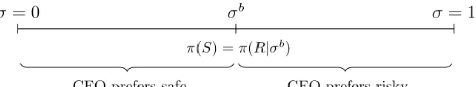
This assumption will also imply that π(G)> π(B). This assumption is necessary because otherwise the CEO will always choose the safe project and the problem of project selection is irrelevant. The expected profit of the risky project for a given signal σ is denoted by π(R|σ) = σπ(G) + (1 −σ)π(B) and it is increasing in the signal observed by the CEO. Therefore, there will be a benchmark cutoff signal, σb_, at which the expected profit from the safe project will be equal to the expected profit from the risky project (π(S) = π(R|σb_{)). So, the CEO will choose the risky project} above σb _{and the safe project below} _σb _{(see figure 2.3).} _σb _{is given by,}

σb = π(S)−π(B)

π(G)−π(B). (2.2)

To resolve the indifference I assume that the CEO prefers the safe project at σb_.

Proposition 1. If the CEO can observe the signal, then she will offer wage wb _and will choose the risky project when her signal is greater than σb _{and the safe project} when her signal is less than or equal to σb_.

The benchmark expected profit, Πb, is given by

Πb = Z σb 0 π(S)dσ+ Z 1 σb π(R|σ)dσ. (2.3)

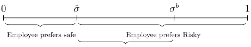
I will now show that given wage wb, the preferred project of the employee is dif-ferent from that of the CEO for some values of σ. In particular, for a range of signals below σb, he prefers the risky project over the safe project. An implication of defini-tion ofσb _{is that at}_σb _{the probability of occurrence of}_X

(23)

0 _σ_ˆ σb 1 Employee prefers safe Employee prefers Risky

Inefficient choice

Figure 2.4: Employee’s preferred project given wage wb

than the safe project.

Lemma 2. At the signal σb_, _{P r}₍_X

2|R, σb)> pS2. Proof: See appendix.

The intuition for the lemma is simple. The probability of occurrence of X0 is positive for risky project and zero for safe project. Since, at σb the expected profits are same, the higher probability of X0 for risky project must be compensated with a higher probability on X2. So at σb, the probability distribution of the profit of risky project is a mean preserving spread of probability distribution of profit of the safe project, i.e. the safe project second order stochastically dominates the risky project. Note that P r(X2|R, σ) increases with sigma.19 For a signal below σb, the CEO prefers the safe project. But in the benchmark wage, the employee receives a positive wage only whenX2 occurs. So just below σb, he will prefer the risky project. In fact, he will prefer the risky project as long asP(X2|R, σ)> pS2. I define ˆσ as the signal at which the probability of X2 is same for the two projects, i.e. P r(X2|R,σˆ) =pS2. So, for σ ∈ [ˆσ, σb], the employee prefers the risky project which is the inefficient project (see figure 2.4).20 Thus there is a conflict between providing incentives for effort and choosing the higher value safe project. This is the standard risk shifting result. Next I analyze the scenario where the CEO does not observe the signal.

B. CEO does not observe the signal

When the CEO does not observe the signal, given that employee’s preference of

19_{P r}₍_X

2|R, σ) =σpG2 + (1−σ)pB2 and pG2 > pB2 because good project first order stochastically dominates the bad project. HenceP r(X2|R, σ) increases withσ.

20_{To resolve indifference, I have assumed that the employee chooses the risky project when he is} indifferent.

(24)

projects differs from that of the CEO’s, she will need to incentivize the employee to choose the efficient project. I will show that in doing so the CEO will have to offer rent to the employee. The CEO’s problem will be to optimally choose a cut off signal,

σc_∈_[ˆ_{σ, σ}b_{], above which the employee chooses the risky project and below which he} chooses the safe project. If the optimal cutoff signal is an interior solution, then the marginal benefit of efficient project choice will be equal to the marginal cost of rent extracted by the employee.

I define pi(σc) as the ex ante probability of occurrence of Xi given cutoff σc. Therefore, pi(σc) = Z σc 0 pS_idσ+ Z 1 σc (σpG_i + (1−σ)pB_i )dσ. (2.4) Given wage contract w, the employee will choose a cutoff signal to maximize his expected wage. This cutoff signal is given by

σc ∈argmax σc

X

i

pi(σc)wi. (2.5)

The first order condition is given by

E[w|S]−(σcE[w|G] + (1−σc)E[w|B]) = 0. (2.6) This has a unique solution for a given wage contract. The term in the brackets is the expected wage from the risky project. So, at the cutoff signal the expected wage from the safe project is same as that from the risky project. The second order condition is given by

E[w|G]−E[w|B]>0. (2.7) The second order condition implies that the expected wage from the risky project is increasing in σ so that above the optimal cut off the employee chooses the risky project.

The wage contract must also satisfy the participation constraint of the employee, that is

X

i

pi(σc)wi ≥u. (2.8)

(25)

maximizes the expected profit, that is the CEO’s objective function is max w,σc_∈_[ˆ_σ,σb_] X i pi(σc)(Xi−wi), (2.9)

such that constraints (2.1), (2.6), (2.7) and (2.8) are satisfied. Recall that wb is the wage contract which offers the minimum expected payment to the employee such that incentive for effort (equation (2.1)) is satisfied. I have also assumed that at this wage the participation constraint is satisfied (see footnote 17). So, any other contract which provides incentive for effort will also satisfy the participation constraint. Therefore, I can ignore the participation constraint of the employee (equation (2.8)).

The problem is solved in two steps. The first step is to find the cheapest contract which implements a given cutoff and also provides incentive to exert effort, i.e. it satisfies equations (2.1) and (2.6). We will see later that the cheapest contract which satisfies these two constraints will also satisfy the second order condition (equation (2.7)). The second step is to find the optimalσc.

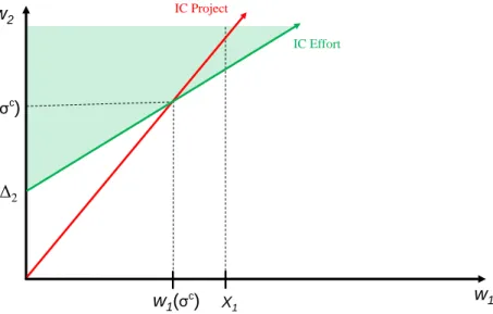
The cheapest contract will havew0 = 0.The reason for this is that ifw0 >0, then a cheaper contract can be found which satisfies constraints (2.6) and (2.1).

Lemma 3. The wage contract which minimizes the expected wage payment and also satisfies constraints (2.1) and (2.6) will have equation (2.1) as a binding constraint and w0 = 0.

Proof: See Appendix.

Given w0 = 0, the IC for effort can be rewritten as

w2 ≥ ∆1 ∆2 w1+ b ∆2 . (2.10)

The IC for cutoff σc, also referred to as IC Project (see figure 2.5), can be rewritten as

M(σc)w1+N(σc)w2 = 0, (2.11) where

M(σc) =pS₁ −P r(X1|R, σc), N(σc) =pS₂ −P r(X2|R, σc).

(26)

Note that M(σc₎_>_{0 and} _N₍_σc₎_<_0.21 _{So, equation (2.11) is a line passing through} origin with a positive slope. For notational simplicity, going forward, I drop the argument σc _{from functions} _M _and _N_{. The cheapest contract is given by the point} of intersection of equations (2.10) and (2.11) (see figure 2.5) and is denoted by

w1(σc) = b/∆2 −M N − ∆1 ∆2 , w2(σc) = w1(σc) ∆1 ∆2 +b/∆2.

Comparing this wage with the benchmark wage, the expected rent extracted by the employee if the CEO incentivizes him to choose σc _{as the cutoff,} _r₍_σc_{), can be} written as

r(σc) = p1(σc)w1(σc) +p2(σc) ∆1 ∆2

w1(σc). (2.12) The rent extracted is positive even for ∆1 < 0, because the cheapest contract which incentivizes effort is wb _{which pays 0 when} _X

1 is realized. Any other contract which satisfies the incentive for effort will pay a higher expected wage, so the rent extracted from any other contract will be positive.

I will now show that the above wage contract also satisfies the second order con-dition (equation (2.7)). The slope of IC project is −M/N and it can be written as22 −M/N = P r(X2|R, σ c₎₋_pS 2 +P r(X0|R, σc) P r(X2|R, σc)−pS2 .

Note that the slope is greater than 1. This implies that at the optimal contract

w2(σc) must be greater than w1(σc) and hence equation (2.7) is automatically satis-fied.23 _{Also note that the slope} ₋_M/N _{is decreasing in} _σc _because _{P r}₍_X

0|R, σc) is decreasing and P r(X2|R, σc) is increasing in σc. At ˆσ, N = 0 so the slope is infinite. The decreasing slope implies that w1(σc) is increasing inσc.

Lemma 4. The slope of constraint (2.11) decreases and w1(σc) increases as σc in-creases.

w1(σc) is increasing in σc because of the following reason. As σc increases,

21_{This is because} _pS

2 < P r(X2|R, σc) in the interval [ˆσ, σb]. Also, M(σc) = −N(σc) + P r(X0|R, σc₎_._{So, it is positive.}

22_M ₌_pS

1 −P r(X1|R, σc). SubstitutingpS1 = 1−pS2 andP r(X1|R, σc) = 1−P r(X2|R, σc)− P r(X0|R, σc_{), we get the expression.}

23_{We have}_w

2(σc)> w1(σc)> w0(σc) = 0, therefore the wage from the good project first order stochastically dominates the wage from the bad project. Hence,E[w|G]> E[w|B].

(27)

IC Effort b/Δ₂ w2 w₁ IC Project X₁ w1(σ c ) w2(σ c )

Figure 2.5: Rent extraction by employee

P r(X2|σc) also increases. Therefore the wage wb which pays only when X2 is re-alized becomes more lucrative for risky project relative to the safe project. The safe project has higher weight on X1 relative to risky project (since M > 0), therefore to compensate for the risky project becoming more lucrative, the CEO will have to increase the wage when X1 is realized. Recall that in the benchmark case, no wage was being paid on the realization of X1. But now the CEO is forced to pay a pos-itive wage to incentivize employees to choose the safe project. This results in rent extraction by the employee relative to the benchmark wage.

Also note that w1(σc) may be greater than X1 (see figure 2.6). If this is so, then the CEO will not be able to implement that σc _{as cutoff. For simplicity I assume} that for all σc ∈ [ˆσ, σb], w1(σc) ≤ X1, that is the CEO can implement any cutoff. This will be true if w1(σb)≤X1 because w1(σc) increases with σc (lemma 4). If this assumption does not hold true then the results will only get stronger.24

The CEO benefits from implementing the cutoff σc _{because now the employee} chooses safe project over the risky one in the interval [ˆσ, σc_{] where the former has}

24_{This is because the CEO will be forced to maximize the profit only over that subset of [ˆ}_{σ, σ}b_]

(28)

IC Effort b/Δ₂ w2 w₁ IC Project X₁ w1(σ c ) w2(σ c )

Figure 2.6: w1(σc)> X1. σc cannot be implemented.

higher expected profits than the latter. This benefit is given by

B(σc) =

Z σc

ˆ σ

[π(S)−π(R|σ)]dσ. (2.13)

Now I solve for the optimal cutoff. The CEO chooses σc _{to maximize the benefit} minus the rent extracted, i.e. optimal cutoff, denoted by σ∗, is given by

σ∗ ∈argmax σc_∈_[ˆ_σ,σb_]

B(σc)−r(σc).

Since here a continuous function is maximized over a closed and bounded interval, an optimal cutoff signal, σc ₌ _σ∗_{, will exist. The marginal benefit} _∂B₍_σc₎_/∂σc _is

π(S)− π(R|σ), which is decreasing in σc _{and at the cutoff} _σb _{it becomes 0. The} marginal cost is ∂r(σc₎_/∂σc _{is always positive (see proof of proposition 2). So,} _σb cannot be the optimal solution.

Proposition 2. There exists an optimal σ∗ ∈ [ˆσ, σb) which maximizes the profit of the CEO.

(29)

The total expected profit, Π∗, is given by

Π∗ = Πb−

Z σb

σ∗

[π(S)−π(R|σ)]f(σ)dσ−r(σ∗).

The first term is the benchmark profit. The second term is loss in profit due to inefficient project choice in interval (σ∗, σb_).25 _{The third term is rent extracted by} the employee. The inefficiency is arising because there is a conflict between giving incentives to the employee to work on the project and choosing the right project ex ante.

But what if the two tasks are split between two employees? Suppose the task of choosing the project is assigned to the risk manager (RM) and the task of exerting effort once the project is chosen is assigned to the trader. As in the real world, the RM may not directly choose the project, but the trader is required to get the ap-proval of the RM before he can invest in any project. The RM has a veto power over any project chosen by the trader and thus has effective control over the choice of the project. In this case the two incentive constraints will be split and I show that more efficient outcomes can be reached. This is because once the tasks are split, the RM will not be able to extract any rents and is only paid his reservation wage. If the reservation wage is small then splitting the tasks may be a more efficient outcome. I analyze these ideas next.

C.Splitting the tasks: Trader and Risk Manager

Suppose there are two employees, a trader and a RM. The trader first proposes a project to the RM. The job of the RM is to approve the project that should be undertaken based on his signal (σRM) about the type of the risky project. σRM is drawn from the same probability distribution as the employee discussed earlier, i.e

σRM ∼ U[0,1]. The trader then exerts effort to execute the chosen project. The reservation wage of both employees is same (u).

Now, since there is no need to incentivize the trader to choose the right project, the CEO will offer him the cheapest wage contract such that he exerts effort. So the wage contract of the trader will be wT = wb = (0,0, b/∆2).26 If the CEO wants the RM

25_{To resolve the indifference I have assumed that the employee chooses the risky project at}_σ∗_.

(30)

Participation Constraint w2 w₁ IC Project X1 Resource Constraint P

Figure 2.7: Risk Manager’s contract is given by point P

to choose a particular cutoff σc_{, then his wage,} _w

RM = (w0,RM, w1,RM, w2,RM), must satisfy incentive constraint (2.6) and the participation constraint (2.8). If the RM is offered zero wage when X0 is realized i.e. w0,RM = 0, equation (2.6) can be written as equation (2.11). This equation then has a postive slope for any σc ∈ [ˆσ, σb] (see figure 2.7). Also, the participation constraint has a negative slope (−p1(σc)/p2(σc)). So any cutoff can be implemented by offering the RM his reservation wage. Hence the CEO will provide incentives to the RM to implement the benchmark cutoff σb and his expected wage payment is u. Note that the exact wage is indeterminate.27 But if w0,RM = 0, then w1,RM = uN p1(σb)N −p2(σb)M , w2,RM = −uM p1(σb)N −p2(σb)M .

The expected profit, ΠRM, is benchmark profit minus the expected wage paid to the RM, i.e.

ΠRM = Πb −u. (2.14)

27_{The IC for}_σc_{(equation 2.6) and participation constraint (equation 2.8) are equations of plane}

in three dimensional coordinate system. Their intersection is a line and not a point. Any wage on this line which satisfies the limited liability constraint and also the resource constraint can be offered to the RM.

(31)

Now comparing ΠRM with Π∗, it is clear that if u is low enough such that

u <

Z σb

σ∗

[π(S)−π(R|σ)]dσ+r(σ∗), (2.15)

then ΠRM >Π∗. So, it is better to have a RM than directly incentivize the trader to choose the right project.

Proposition 3. If u is low enough such that (2.15) is satisfied, it is more profitable to rely on the RM to chooses the efficient project than directly offer incentives to the trader.

Note that having a RM not only increases the profit, but is also socially efficient. From the perspective of the social planner, the rent, r(σ∗), is merely a transfer from the bank to the employee. But there is also a loss in efficiency because the less profitable project gets chosen in the interval [σ∗, σb_{] which the social planner would} not prefer. Thus, having a RM is not only profit maximizing but also increases social welfare.

The RM may not have as accurate signal as the trader. But even if the RM’s signal is more noisy, it may be more efficient to rely on the him. Suppose that with probabilityz, the RM receives the same informative signal, but with probability 1−z, his signal is a pure noise drawn from uniform distribution. Then a corollary of propo-sition 3 is that as long as z is close enough to 1, it is still better to have a RM. This will be true because any loss will be proportional to (1−z)

Corollary: Having a RM is more efficient as long as z is close to 1.

D. Discussion

Financial institutions make investments which are information sensitive. To re-solve this information problem, they delegate the task of information acquisition to their employee such as loan officers, insurance officers and traders. The process of information acquisition and the optimal actions conditional on them is dynamically determined. Making investment decisions conditional on the information available is only the first step. After the investment decisions are taken, the employees have to

(32)

constantly exert effort to make those investments successful. Banks use the technol-ogy of ‘relationship lending’ (see Berger and Udell (2002)), in which the loan officers monitor their portfolio of loans and gather information about them. Traders have to exert effort to execute the trade and then monitor their portfolio so that they are able to liquidate or hedge their positions on time in case the situation deteriorates. This paper argues that there is an inherent conflict between incentivizing an employee to take the information sensitive step of deciding which investment to make and then continuously exert effort to make those investments successful.

I show that, to resolve this conflict, the banks have to rely on separate RMs to monitor their employees. RMs first get involved at the initial step in which they approve the investments. But risk management task does not stop there. They may keep monitoring the portfolio to check that their employees are taking the requisite action. For example, banks use loan review process so that they are able to monitor the loan officers (see Udell (1989)). A loan officer may receive information based on which the optimal safe decision could be to liquidate a loan early. But given his high powered contract, he may find it optimal to choose the risky option of not liquidating the loan hoping for a positive outcome in future. A loan review process would prevent such decisions. My paper thus provides an explanation for having separate agents as RMs.

In my model, the optimal contract offers the risk takers high powered incentives without worrying about their incentive to indulge in risk shifting. This provides an important insight regarding the debate on compensation contracts of bank employees which has been happening since the financial crisis. While a lot of blame has been assigned to the traders who were taking excessive risk incentivized by their high bonus contracts, there has been less focus on the role of RMs. But as per the institutional hierarchy, it is the RMs who are in charge of the investment decisions. The RMs at UBS prevented their traders from making investments in CDOs only in May of 2007 (UBS (2008)). But if they had taken this decision earlier, then the bank would have suffered much smaller losses. Since the RMs are ultimately in charge of approving the investment decisions, any blame for the crisis has to be equally shared by them or the CEOs who may have ignored the RMs’ suggestions. I turn to this issue next.

(33)

2.4

Risk Averse Risk Manager

I have shown that having a separate RM, who has a veto power over what project can be chosen is optimal. While at the lower levels of hierarchy, the RMs do enjoy a veto power, at the highest level they play more of an advisory role to the CEO and make recommendations regarding investment strategies. As mentioned in the introduction, there are numerous anecdotal evidences where the CEOs ignored their RMs partic-ularly before the recent global financial crisis. So the question that arises is that if RMs are important, then why does the CEO ignore them when they recommend the safe investment strategy and goes ahead with the risky investment strategy? In this section, I show that if the RM is risk averse, then there will be overinvestment in the safe project. In such a case, it may not be optimal for the CEO to always agree with the RM. In particular, the CEO may be better off by occasionally ignoring the RM when he suggests the safe project. But if the RM suggests the risky project then the CEO always agrees with him.

A. Optimal contracting with risk averse risk manager when CEO doe not ignore him

To simplify the analysis I will continue to assume that the trader is risk neutral and is therefore offered benchmark wage wb_{. The RM is risk averse with utility} function U such that U0 > 0, U00 < 0 and U0(0) is infinite. His reservation utility is still denoted by u. I definew as the wage which gives him his reservation utility, i.e.

U(w) =u.

Now there can be two cases, (i.) X0 ≥ w and (ii.) X0 < w. If X0 > w, then full risk sharing is possible, that is the CEO can pay the RM a fixed wage w and ask him to choose the benchmark cutoff σb. Since the RM gets paid the same wage in all states, he will have no incentive to deviate. But ifX0 < w, then the CEO cannot offer full risk sharing contract to the RM. In this case, the RM may be biased towards investing in the safe project. I will later argue that there may be over investment in safe project even when full sharing is possible when there are reputation concerns for the RM. I first analyze the case when full risk sharing is not possible.

Suppose the CEO offers wage contract to the RM to incentivize him to choose a cutoff σc_{. Analogous to equation (2.6), the incentive compatibility constraint to}

(34)

choose this cutoff can now be written as

E[U(wRM)|S]−(σcE[U(wRM)|G] + (1−σc)E[U(wRM)|B]) = 0. (2.16) At the cutoff the expected utility from the risky project equals the expected utility from the safe project. The second order condition is

E[U(wRM)|G]−E[U(wRM)|B]>0. (2.17) This constraint implies that the expected utility from risky project is increasing in signal observed by the RM. If this constraint is satisfied then the first order condition (2.16) is necessary and sufficient for the RM to chooseσc as the cutoff. I will assume that the second order condition holds true.28 It will be true ifw2,RM > w1,RM because it implies that E[U(wRM)|G] > E[U(wRM)|S], and since in any solution (2.16) is satisfied, so (2.17) must hold true.

The participation constraint can now be written as

X

i

pi(σc)U(wi,RM)≥u. (2.18)

The CEO’s problem is to chooseswRM and σc such that they maximize the expected profit, i.e. max σc_,w RM X i pi(σc)(Xi−wRM,i)−p2(σc)b/∆2, (2.19) such that constraints (2.16), (2.17) and (2.18) are satisfied.

I show that the optimal cutoff signal in this case may be greater than σb _which implies over investment in the safe project. If the safe project has high weight on

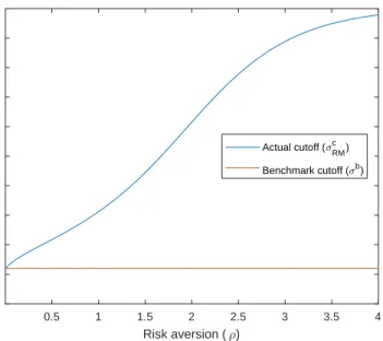
X1, i.e. pS1 is high, then the variance of safe project will be very low. In this case compensating the RM with the safe project will be cheaper than compensating him with the risky project. Recall that at σb_{, the expected profit from the safe and risky} project when benchmark wage is paid to the trader is same, i.e. π(S) = π(R|σb_). So, if the CEO chooses the marginally greater cutoff than σb, then the marginal cost is zero but the marginal benefit is positive because compensating the RM with safer project is cheaper. Hence the CEO finds it optimal to overinvest in the safe project relative to the benchmark case and the optimal cutoff for the RM, σc

RM, is greater

(35)

0.5 1 1.5 2 2.5 3 3.5 4 Risk aversion ( ) 0 0.1 0.2 0.3 0.4 0.5 0.6 0.7 0.8 0.9 1 Cutoff signal Actual cutoff ( c_RM) Benchmark cutoff ( b) Figure 2.8: σc

RM as a function of risk aversion (ρ)

than σb. The next proposition summarizes this result. For the exact condition on how high pS₁ must be to get the result, see the proof of the proposition.

Proposition 4. IfpS

1 is large enough then the risk manager’s cutoff signalσRMc > σb. Proof: See Appendix.

B. An Example

Consider the following parameter values. X2 = 100,X1 = 10, X0 = 1, b/∆2 = 40,

pG₂ = 0.8,pG₁ = 0.2, pS₂ = 0.9,pS₁ = 0.1,pB₂ = 0.03, p₁B = 0.75, pB₀ = 0.2. The RM has CRRA utility function c1₁−₋ρ−_ρ1. These parameter values implies that the benchmark cutoff σb _{= 0}_._{109. If the risk aversion (}_ρ_{) increases then it is costlier to compensate} the RM with the risky project relative to the safe project. So the actual cutoff (σc

RM) will be higher. This is shown in figure 2.8. Note that when ρ = 0, then the actual cutoff is equal to benchmark cutoff.

C. CEO may ignore the risk manager when he suggests safe project

(36)

that the CEO may find it optimal to ignore the RM when he suggests the safe project and instead invests in the risky project. But if the RM suggests the risky project then the CEO agrees with him. I denote by q the probability that the CEO ignores the RM whenever he suggest the safe project. Then theex ante probability of occurrence of Xi depends on σc and q, and it is denoted by pi(σc, q) which can be expressed as

pi(σc, q) = (1−q) Z σc 0 pS_idσ+q Z σc 0 P r(Xi|R, σ)dσ+ Z 1 σc P r(Xi|R, σ)dσ.

Analogous to (2.18), the participation constraint of the RM is

X

i

pi(σc, q)U(wi,RM)≥u. (2.20)

The incentive constraint to implementσc_{is same as (2.16) and second order condition} is same as (2.17).29 _{The CEO’s objective is}

max σc_,w RM,q X i pi(σc, q)(Xi−wRM,i)−p2(σc, q)b/∆2, (2.21)

such that (2.16), (2.17) and (2.20) are satisfied. The optimal q and σc _{are denoted} byq_RM∗ and σ_RM∗ . I get the following result.

Proposition 5. If X2 is large relative to X1, pS1 is close enough to 1 and risk aver-sion is neither small nor large, then q_RM∗ >0.

Proof: See appendix.

The intuition for this proposition is as following. Since pS

1 is large, so according to proposition 4, the cutoff signal when CEO does not ignore RM (σc

RM) is above first best cutoff σb_{. If}_X

2 is large relative toX1 and pS1 is large, thenπ(G) is large relative toπ(S). This implies that σb _{is small (see equation (2.2)).}

When the CEO ignores the RM and chooses the risky project instead of the safe project, then it is inefficient decision forσRM ∈[0, σb]. So, ifσb is small, then the cost of ignoring the RM will be small. Risk aversion has two opposing effects. First, as risk aversion increases, σ_RMc also increases. So, the interval [σb, σc_RM] in which inefficient

29_{At the cutoff the RM is indifferent between safe and risky project. This can be written as} qE[U(w)|S] + (1−q)E[U(w)|R, σc] =E[U(w)|R, σc] which is same as equation (2.16). Similarly the second order condition is also the same.

(37)

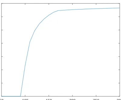
50 100 150 200 250 300 X 2 0 0.1 0.2 0.3 0.4 0.5 0.6 0.7 Probability of ignoring

Figure 2.9: Probability of ignoring risk manager as function of X2

safe project is recommended by the RM increases. Thus the benefit of ignoring the RM will be larger. But there is a cost of ignoring the RM as well which is that the CEO now has to compensate him with the risky project more often which is costlier for the CEO. This cost increases as risk aversion increases. So if X2 is high relative to X1, and risk aversion is neither very low or nor very high, then CEO will ignore the RM.

D. Example continued

Figure 2.9 shows that as X2 increases, the probability that the CEO will ignore the RM increases. The figure has been calculated assuming ρ = 2.5. The CEO is effectively playing a mixed strategy, i.e. when the RM recommends the safe project she ignores his proposal with some probability and accepts with complementary prob-ability.

Figure 2.10 shows the probability of ignoring the RM when he recommends the safe project as a function of risk aversion (ρ). When ρ is low, then the interval [σb_{, σ}c

(38)

0.5 1 1.5 2 2.5 3 3.5 Risk aversion ( ) 0 0.1 0.2 0.3 0.4 0.5 0.6 0.7 0.8 0.9 1 Probability of ignoring

Figure 2.10: Probability of ignoring risk manager as function of ρ

is taken is small and the CEO does not find it optimal to ignore the RM and pay the extra cost of compensating him with risky project. But asρbecomes larger CEO finds it optimal to ignore the RM. At high values of ρ, compensating the RM with risky project is very costly, so again the CEO does not ignore him.

2.5

Multiple Risk Managers and Coordination

Prob-lem

I have discussed one reason for failure of risk management, which is that the CEO may ignore the RMs when he suggests the safe project. I now discuss another reason why risk management may fail. The second reason for risk management failure may have been that the RMs in the banks may not have disclosed their information to the CEOs. Paul Moore, the ex-head of Group Regulatory Risk at HBOS, in his memorandum said:30

I am quite sure that many many more people in internal control

(39)

tions, non-executive positions, auditors, regulators who did realise that the Emperor was naked but knew if they spoke up they would be labelled “trouble makers” and “spoil sports” and would put themselves at personal risk.

The statement suggests that many people in risk management and control func-tions may not have come forward and warned the CEO about the risks involved in the bank’s investment strategy. I extend the model where there are multiple RMs and show that there can be coordination problem in disclosure of information to the CEO even when they have been offered incentive compatible contracts to do so.

To illustrate the coordination problem I make some changes in the model. The bank now has two RMs.31 _{They differ in their ability and are of two kinds, smart} with probabilityβ and incompetent with probability (1−β). The RMs do not know whether they are smart or incompetent. Each RM privately observes a signal about the type of risky project with probabilityψRM and he does not observe any signal with probability (1−ψRM). I assume that the signals are discrete rather than continuous. The signal can take two values, low(l) andhigh (h). Observing no signal is denoted byn. The smart RM observes perfectly accurate signal when he see it, i.e.

P r(h|G,smart sees) =P r(l|B,smart sees) = 1.

The incompetent RM observes noisy signals with accuracy z ∈(1/2,1) when he sees it, i.e.

P r(h|G,incompetent sees) =P r(l|B,incompetent sees) =z.

The assumption z ∈ (1/2,1) implies that the signal seen by a RM, with the prior that he is incompetent with probability 1−β, is informative as well. I will refer to the signal seen by the RM (n, h or l) as the type of the RM.32 The signal observed by first (second) RM is denoted by σ1 (σ2).

I assume that the CEO also privately observes the signal (high or low), denoted by σCEO, with probability ψCEO, and does not observe any signal with probability (1−ψCEO). The CEO is always smart and like the smart RM observes perfectly accurate signal when she sees it. The CEO knows that she is smart. So when she

31_{The model can be generalized to any number of RMs.}

32_{This is not to be confused with the ability of the RM. I do not refer to different abilities of the} RM as his type because the risk manger does not know his ability where as in incomplete information games we assume that an agent knows his type.

(40)

observes the signal, she knows whether the risky project is good or bad. But when she does not observe any signal, then she has to rely on the signal disclosed by the RMs. After he discloses his signal, the CEO updates her beliefs about the RM being incompetent. If the RM discloses a signal opposite of that seen by the CEO, i.e. if he discloses low signal (high signal) when the CEO has seen the high signal (low signal), then the CEO is able to learn that the RM is incompetent. In this case the CEO may fire the RM. When the RMs discloses no signal, the CEO can never be sure that the RM is incompetent and may not replace him. So this provides an incentive to the RM to lie and disclose that he has not observed any signal. Hence the CEO needs to provide incentives to him to disclose the signal. I make the following assumption.

Assumption 2.

i. If the RM discloses the opposite signal as that seen by the CEO, then he is fired and does not receive any wage.

ii. If he discloses that he has not observed any signal, then he is retained.

iii. If the CEO does not observe any signal, then she does not replace the RM irre-spective of the signal he discloses.

The assumption can be justified as following. There may be an expected continua-tion value of keeping the RM depending on the posterior belief that he is incompetent. There is also a cost of replacing him.33 _{Here assumption 2 says that if the CEO is sure} that the RM is incompetent, then the continuation value of keeping an incompetent RM is less than the replacement cost. On the other hand, when the CEO knows that the RM has either seen no signal or seen the opposite signal, then the posterior that he is incompetent is less than 1.34 In this case the expected continuation value is more than the replacement cost. Similarly if the CEO does not observe any signal, then she cannot be sure that the RM is incompetent, and therefore he is not replaced. When the CEO does not observe any signal then she has to rely on the signals of the RM. The coordination problem in disclosure of low signal will exist at high values

33_{The replacement cost could be the cost of posting an advertisement to hire a new RM or the} cost of training a new RM.

34_{When the CEO observes a signal, say}_h₍_l_{) and she knows that the employee has either seen no} signal or has seen the opposite signal l (h), then she is not sure that the employee is incompetent. The probability that he is incompetent is (1−β)((1−β) +β(1−ψRM

1−ψRMβ))

(41)

of α. I make the following assumption on α.

Assumption 3. α is high such that the CEO chooses the safe project only when both RMs have seen the low signal. If the CEO knows that one manager has observed low signal and the other has not observed any signal then she prefers the risky project.

Given these assumptions it can be shown that a full separating equilibrium in which each type of employee discloses truthfully cannot exist. The reason for this is that when a RM observes the high signal, he knows that the CEO (when σCEO=n), will choose the risky project whether he discloses h or deviates and disclose n, irre-spective of the signal disclosed by other employee. But if he discloses h, then there is a chance that he will get fired if the CEO observes the low signal. Thus the htype employee will never disclose.

Lemma 5. Given assumptions 2 and 3, a separating equilibrium cannot exist. Proof: See appendix.

The set of equilibrium that may exist are described in table 2.2. The pair of signals observed the RMs is called a node. ‘Pooling LL’ is the equilibrium in which RMs disclose the low signal but not the high signal. It is a pooling equilibrium because theh

type RM does not disclose and pools with then type. Pooling NN is the equilibrium where the l type also does not disclose. Although separating equilibrium can not be implemented, Pooling LL is efficient equilibrium because the CEO takes efficient decisions regarding the project choice.35 _{Pooling NN is the inefficient equilibrium} because CEO invests in the risky project even when both RMs observe low signal.

Since the CEO wants to make efficient decisions, she will design contracts to implement Pooling LL. Note that in Pooling LL, CEO prefers the safe project only when both employees disclosel and not otherwise.

As in the one RM, case it can be shown using very similar analysis that his participation constraint is binding. I do not repeat the analysis again. Here I focus on another friction, that is the coordination problem in disclosure of signals, which

35_{Although these equilibria are efficient with respect to project choice, they are less efficient than} the separating equilibrium because separating equilibrium will result in efficient firing of employee which does not happen in Pooling LL. For example, if an employee observes h, then he does not disclose in Pooling LL and does not get fired even when CEO observesl.

(42)

Equilibrium Nodes RM Disclosure Project choice Pooling LL

ll ll Safe

lh/hl, ln/nl ln/nl Risky

hh, hn/nh,nn nn Risky

Pooling NN all nn Risky

Table 2.2: Pooling equilibrium with two employees

will exist in spite of incentive compatible contracts. I will show that whenever Pooling LL exists, Pooling NN will also exist. This is the coordination problem where multiple equilibrium can exist together.

The reason for coordination problem is that there is strategic complementarity in disclosure strategy of the employees. If assumption 3 holds, then the CEO will be convinced to choose the safe project only if both disclosel and not otherwise. If only one RM discloses then he only risks the chance of getting fired if the CEO observes

h without changing her decision if she observes n. So if one employee believes that the other will not disclose then he is better off not disclosing his signal as well. Thus, whenever Pooling LL will exist Pooling NN will also exist.

Proposition 6. Even if the CEO designs contracts to implement Pooling LL, if as-sumptions 2 and 3 hold, then Pooling NN will always exist alongside Pooling LL. Proof: See appendix.

This result is similar to Diamond and Dybvig (1983), where we also have a coor-dination problem in spite of having incentive compatible contracts. In their paper, there are strategic complementarities between actions of the late consumers. If one late consumer believes that the others will run on the bank then he is better off withdrawing as well resulting in the inefficient bank run equilibrium.

I have shown that for coordination problem to exist, the beliefs have to be more extreme in the sense that it requires both employees to disclose the same signal to convince the CEO to take a

Essays On Banking