ISSUES IN SPATIAL DATABASES AND GEOGRAPHIC INFORMATION SYSTEMS (GIS) HANAN SAMET

Copyright © 2007 Hanan Samet

These notes may not be reproduced by any means (mechanical or elec-tronic or any other) without express written permission of Hanan Samet

ISSUES IN SPATIAL DATABASES AND GEOGRAPHIC

INFORMATION SYSTEMS (GIS)

H

ANAN

S

AMET

C

OMPUTER

S

CIENCE

D

EPARTMENT AND

C

ENTER FOR

A

UTOMATION

R

ESEARCH AND

I

NSTITUTE FOR

A

DVANCED

C

OMPUTER

S

TUDIES

U

NIVERSITY OF

M

ARYLAND

PRINCE GEORGES COUNTY

BACKGROUND (A PERSONAL VIEW!)

1.

GIS originally focussed on paper map as output

• anything is better than drawing by hand

• no great emphasis on execution time

2.

Paper output supports high resolution

• display screen is of limited resolution

• can admit less precise algorithms

• Ex: buffer zone computation (spatial range query)

a. usually use a Euclidean distance metric (L

2

)

• takes a long time

b. can be sped up using a quadtree and a

Chessboard distance metric (L

∞

)

• not as accurate as Euclidean — but may not

be able to perceive the difference on a display

screen!

• as much as 3 orders of magnitude faster

3.

Users accustomed to spreadsheets

• GIS should work like a spreadsheet

• fast response time

• ability to ask “what if” questions and see the

results

• incorporate a database for seamless integration of

spatial and nonspatial (i.e., attribute data)

zk9

GENERAL SPATIAL DATABASE ISSUES

1.

Why do we want a database?

• to store data so that it can be retrieved efficiently

• should not lose sight of this purpose

2.

How to integrate spatial data with nonspatial data

3.

Long fields in relational database are not the answer

• a stopgap solution as just a repository for data

• does not aid in retrieving the data

• if data is large in volume, then breaks down as

tuples get very large

4.

A database is really a collection of records with fields

corresponding to attributes of different types

• records are like points in higher dimensional space

a. some adaptations take advantage of this analogy

b. however, can act like a straight jacket in case of

relational model

5.

Retrieval is facilitated by building an index

• need to find a way to sort the data

• index should be compatible with data being stored

• choose an appropriate zero or reference point

• need an implicit rather than an explicit index

a. impossible to foresee all possible queries in

advance

b. explicit would sort two-dimensional points on

the basis of distance from a particular point P

• impractical as sort is inapplicable to points

6.

Identify the possible queries and find their analogs in

conventional databases

• e.g., a map in a spatial database is like a relation in

a conventional database (also known as spatial

relation)

a. difference is the presence of spatial attribute(s)

b. also presence of spatial output

7.

How do we interact with the database?

•

SQL

may not be easy to adapt

• graphical query language

• output may be visual in which case a browsing

capability (e.g., an iterator) is useful

8.

What strategy do we use in answering a query that

mixes traditional data with nontraditional data?

• need query optimization rules

• must define selectivity factors

a. dependent on whether index exists on

nontraditional data

b. if no, then select on traditional data first

• Ex: find all cities within 100 miles of the Mississippi

River with population in excess of 1 million

a. spatial selection first if region is small (implies

high spatial selectivity)

b. relational selection first if very few cities with a

large population (implies high relational

zk11

DATA IN SPATIAL DATABASES

1.

Spatial information

• locations of objects (are discrete, individual points

in space)

• space occupied by objects (are continuous; have

extent)

a. example objects

• lines (e.g., roads, rivers)

• regions (e.g., buildings, crop maps,

polyhedra)

• others ...

b. are objects disjoint or may they overlap?

• e.g., several crop types may be grown on a

plot of land

• not concerned here with raster vs: vector issues

as these are data

representation issues rather

than data

type issues

2.

Non-spatial information

• region names, postal codes, ...

• city population, year founded, ...

• road names, speed limits, ...

EXAMPLE QUERIES ON LINE SEGMENT DATABASES

• Queries about line segments

1. All segments that intersect a given point or set of

points

2. All segments that have a given set of endpoints

3. All segments that intersect a given line segment

4. All segments that are coincident with a given line

segment

• Proximity queries

1. The nearest line segment to a given point

2. All segments within a given distance from a given

point (also known as a range or window query)

• Queries involving attributes of line segments

1. Given a point, find the closest line segment of a

particular type

2. Given a point, find the minimum enclosing polygon

whose constituent line segments are all of a given

type

3. Given a point, find all the polygons that are incident

on it

gs10

WHAT MAKES CONTINUOUS SPATIAL DATA

DIFFERENT

1.

Spatial extent of the objects is the key to the

difference

2.

A record in a DBMS may be considered as a point in

a multidimensional space

• a line can be transformed (i.e., represented) as a

point in 4-d space with (

x

₁

,

y

₁

,

x

₂

,

y

₂

)

(

x

2

,

y

2

)

(

x

1

,

y

1

)

• good for queries about the line segments

• not good for proximity queries since points outside

the object are not mapped into the higher

dimensional space

• representative points of two objects that are

physically close to each other in the original space

(e.g., 2-d for lines) may be very far from each other

in the higher dimensional space (e.g., 4-d)

A

B

• Ex:

• problem is that the transformation

only transforms the space occupied

by the objects and not the rest of the

space (e.g., the query point)

• can overcome by projecting back to original space

3.

Use an index that sorts based upon spatial

SPATIAL INDEXING REQUIREMENTS

1.

Compatibility with the data being stored

2.

Choose an appropriate zero or reference point

3.

Need an implicit rather than an explicit index

• impossible to foresee all possible queries in

advance

• cannot have an attribute for every possible spatial

relationship

a. derive adjacency relations

b. 2-d strings capture a subset of adjacencies

• all rows

• all columns

• implicit index is better as an explicit index which,

for example, sorts two-dimensional data on the

basis of distance from a given point is impractical

as it is inapplicable to other points

• implicit means that don't have to resort the data for

queries other than updates

gs11

SORTING ON THE BASIS OF SPATIAL OCCUPANCY

• Decompose the space from which the data is drawn into

regions called

buckets

(like hashing but preserves order)

• Interested in methods that are designed specifically for

the spatial data type being stored

• Basic approaches to decomposing space

1. minimum bounding rectangles

• e.g.,

R

-tree

• good at distinguishing empty and non-empty

space

• drawbacks:

a. non-disjoint decomposition of space

• may need to search entire space

b. inability to correlate occupied and unoccupied

space in two maps

2. disjoint cells

• drawback: objects may be reported more than once

• uniform grid

a. all cells the same size

b. drawback: possibility of many sparse cells

• adaptive grid — quadtree variants

a. regular decomposition

b. all cells of width power of 2

• partitions at arbitrary positions

a. drawback: not a regular decomposition

b. e.g.,

R+

-tree

• Can use as approximations in filter/refine query

processing strategy

MINIMUM BOUNDING RECTANGLES

Objects grouped into hierarchies, stored in a structure

similar to a B-tree

Object has single bounding rectangle, yet area that it

spans may be included in several bounding rectangles

Drawback: not a disjoint decomposition of space

Examples include the R-tree and the R*-tree

a b c d e f g h i

Order (

m

,

M

) R-tree

1. between

m

M

/2 and

M

entries in each node

except root

2. at least 2 entries in root unless a leaf node

R3 R4 R5 R6 R4 R3 R5 R6 R1 R2 R2: R1: R2 R1 R0: R0

hi32

SEARCHING FOR A POINT OR LINE

SEGMENT IN AN R-TREE

1 b b a d g h c i e f R2 R1 R4 R3 R5 R6 a b c d e f g h i R3 R4 R5 R6 R2 R1 Q

Drawback is that may have to examine many nodes

since a line segment can be contained in the covering

rectangles of many nodes yet its record is contained in

only one leaf node (e.g., i in R2, R3, R4, and R5)

Ex: Search for a line segment containing point Q

R3: R4: R5: R6: R1: R2: R0: R0

hi32

Q is in R0

2 v

hi32

Q can be in both R1 and R2

3 r

hi32

4 z

Searching R1 first means that R4 is searched but this

leads to failure even though Q is part of i which is in R4

hi32

5 g

Objects decomposed into disjoint subobjects; each

subobject in different cell

Drawback: in order to determine area covered by

object, must retrieve all cells that it occupies

Techniques differ in degree of regularity

R+-tree (also k-d-B-tree) and cell tree are examples

of this technique

a b c d e f g h i Q R3 R4 R6 R5 h g d c h i c f i a b e i R3: R4: R5: R6: R4 R3 R5 R6 R1 R2 R1: R2: R2 R1 R0: R0

hi33.1

K-D-B-TREES

a b c d e f g h i 1 b Q

• Rectangular embedding space is hierarchically

decomposed into disjoint rectangular regions

• No dead space in the sense that at any level of the tree,

entire embedding space is covered by one of the nodes

• Blocks of k-d tree partition of space are aggregated into

nodes of a finite capacity

• When a node overflows, it is split along one of the axes

• Originally developed to store points but may be extended

to non-point objects represented by their minimum

bounding boxes

• Drawback: in order to determine area covered by object,

must retrieve all cells that it occupies

hi33.1

2 r R3 R4 R6 R5

hi33.1

3 z R4 R3 R5 R6 R1 R2 R1: R2:

hi33.1

4 g R2 R1 R0: R0

UNIFORM GRID

Ideal for uniformly distributed data

Supports set-theoretic operations

Spatial data (e.g., line segment data) is rarely uniformly

distributed

hi35

QUADTREES

• Hierarchical variable resolution data structure based on

regular decomposition

• Many different decomposition schemes and applicable

to different data types:

1. points

2. lines

3. regions

4. rectangles

5. surfaces

6. volumes

7. higher dimensions including time

• changes meaning of nearest

a. nearest in time,

OR

b. nearest in distance

• Can handle both raster and vector data as just a spatial

index

• Shape is usually independent of order of inserting data

• Ex: region quadtree

• A decomposition into blocks

— not necessarily a tree!

REGION QUADTREE

• Repeatedly subdivide until obtain homogeneous region

• For a binary image (

BLACK

≡

1 and

WHITE

≡

0)

• Can also use for multicolored data (e.g., a landuse

class map associating colors with crops)

• Can also define data structure for grayscale images

• A collection of maximal blocks of size power of two

and placed at predetermined positions

1. could implement as a list of blocks each of which

has a unique pair of numbers:

• concatenate sequence of 2 bit codes

correspond-ing to the path from the root to the block’s node

• the level of the block’s node

2. does not have to be implemented as a tree

• tree good for logarithmic access

• A variable resolution data structure in contrast to a

pyramid (i.e., a complete quadtree) which is a

multiresolution data structure

A B C D E NW NE SW SE F G H I J L M N O Q K P 37 38 39 40 57 58 59 60 0 0 0 0 0 0 0 0 0 0 0 0 0 0 0 0 0 0 0 0 0 1 1 1 0 0 0 0 1 1 1 1 0 0 1 1 1 1 1 1 0 0 1 1 1 1 1 0 0 0 1 1 1 1 0 0 0 0 1 1 1 1 0 0 B 60 37 L J Q G F H N I O M 57 58 59 40 39 38

hi37

PYRAMID

• Internal nodes contain summary of information in

nodes below them

• Useful for avoiding inspecting nodes where there could

be no relevant information

c1 c2 c3 c4 c5 c6 {c1,c2,c3,c4,c5,c6} {c2,c3,c6} {c2,c3,c4,c5} {c1,c2,c3, c4,c5,c6} {c6}

QUADTREES VS. PYRAMIDS

• Quadtrees are good for location-based queries

1. e.g., what is at location

x

?

2. not good if looking for a particular feature as have to

examine every block or location asking “are you the

one I am looking for?”

• Pyramid is good for feature-based queries — e.g.,

1. does wheat exist in region

x

?

• if wheat does not appear at the root node, then

impossible to find it in the rest of the structure and

the search can cease

2. report all crops in region

x

— just look at the root

3. select all locations where wheat is grown

• only descend node if there is possibility that wheat is

in one of its four sons — implies little wasted work

• Ex: truncated pyramid where 4 identically-colored sons

are merged

c1 c2 c3 c4 c5 c6 {c1,c2,c3,c4,c5,c6} {c2,c3,c6} {c2,c3,c4,c5} {c1,c2,c3, c4,c5,c6} {c6} {c2,c3,c5} {c1,c2,c3,c5}

• Can represent as a list of leaf and nonleaf blocks (e.g.,

as a linear quadtree)

PR QUADTREE (Orenstein)

b1

hp9

Regular decomposition point representation

Decomposition occurs whenever a block contains more

than one point

Useful when the domain of data points is not discrete

but finite

(0,100) (100,100) (100,0) (0,0) (35,42) Chicago

Maximum level of decomposition depends on the

minimum separation between two points

• if two points are very close, then decomposition can be

very deep

• can be overcome by viewing blocks as buckets with

capacity

c

and only decomposing the block when it

contains more than

c

points

1.

2.

3.

4.

Ex:

c

= 1

2 r

hp9

(52,10) Mobile 3 z

hp9

(62,77) Toronto 4 g

hp9

(82,65) Buffalo 5 v

hp9

(5,45) Denver 6 g

hp9

(27,35) Omaha 7 z

hp9

(85,15) Atlanta 8 r

hp9

(90,5) Miami

Use of quadtree results in pruning the search space

Ex: Find all points within radius

r

of point A

A

r

If a quadrant subdivision point

p

lies in a region

l

, then

search the quadrants of

p

specified by

l

1. SE

6. NE

11. All but SW

2. SE, SW

7. NE, NW

12. All but SE

3. SW

8. NW

13. All

4. SE, NE

9. All but NW

5. SW, NW

10. All but NE

1

2

3

9

10

13

12

11

4

5

8

7

6

hp11

FINDING THE NEAREST OBJECT

• Ex: find the nearest object to

P

1 b P 12 8 7 6 13 9 1 4 5 2 3 10 11 D E C F A B

• Assume

PR

quadtree for points (i.e., at most one point

per block)

• Search neighbors of block 1 in counterclockwise order

• Points are sorted with respect to the space they occupy

which enables pruning the search space

• Algorithm:

hp11

2

r

1. start at block 2 and compute distance to

P

from

A

hp11

3 z

2. ignore block 3 whether or not it is empty as

A

is closer

to

P

than any point in 3

hp11

4

g

3. examine block 4 as distance to

SW

corner is shorter

than the distance from

P

to

A

; however, reject

B

as it is

further from

P

than

A

hp11

5

v

4. ignore blocks 6, 7, 8, 9, and 10 as the minimum

distance to them from

P

is greater than the distance

from

P

to

A

hp11

6 z

5. examine block 11 as the distance from

P

to the southern

border of 1 is shorter than the distance from

P

to

A

;

however, reject

F

as it is further from

P

than

A

hp11

7

r

a

PM1 QUADTREE

DECOMPOSITION RULE:

Partitioning occurs when a block contains more than

one segment unless all the segments are incident at

the same vertex which is also in the same block

Vertex-based (one vertex per block)

Shape independent of order of insertion

b

c

d

e

f

g

h

i

cd35

a

PMR QUADTREE

1

Split a block

once

if upon insertion the number of

segments intersecting a block exceeds

N

b

• Edge-based

• Avoids having to split many times when two vertices or

lines are very close as in PM1 quadtree

• Probabilistic splitting and merging rules

• Uses a splitting threshold value — say

N

DECOMPOSITION RULE:

Merge a block with its siblings if the total number of line

segments intersecting them is less than

N

• Merges can be performed more than once

• Does not guarantee that each block will contain at

most

N

line segments

• Splitting threshold is not the same as bucket capacity

Ex:

N

= 2

cd35

2 r b

cd35

3 z c

cd35

d 4 g

cd35

5 v e

cd35

f 6 r

cd35

g 7 z

cd35

h 8 g

cd35

i 9 v

ADVANTAGES OF EDGE-BASED METHODS

The decomposition is focussed where the line segments

are the densest

Handles the situation that several non-intersecting lines

are very close to each other

Able to represent nonplanar line segment data

Good average behavior in terms of node occupancy

Example:

CONSISTENCY OF PM APPROACH

cd47

Stores lines exactly

Each line segment is represented by a pointer to a

record containing its endpoints

Updates can be made in a consistent manner - i.e.,

when a vector feature is deleted, the database can be

restored to the state it would have been in had the

deleted feature never been inserted

Uses the decomposition induced by the quadtree to

specify what parts of the line segments (i.e., q-edges)

are actually present

1. not a digitized representation

2. no thickness associated with line segments

The line segment descriptor stored in a block only

implies the presence of the corresponding q-edge - it

does not mean that the entire line segment is present

as a lineal feature

Useful for representing fragments of lines such as

those that result from the intersection of a line map with

an area map

Ex:

1 b 2 r

cd47

3 z

cd47

MAXIMAL SEARCH RADIUS

P

Properties of the PM quadtree family (PM1, PMR, etc.)

greatly localize the search area for nearest line segment

Assume that the query point P falls in the SW corner of

the small highlighted block

By virtue of the existence of a block of this size, we are

guaranteed that at least one of the remaining

siblings contains a line segment

cd59

NEAREST LINE SEGMENT ALGORITHM

A four stage intelligent search process

Maximal search radius equal to length of parent node's

diagonal

Basic algorithm:

Search the block containing the query point

1.

1

b 2

Search the three siblings

2.

r

cd59

3

Search the three regions of size equal to that of the

parent that are incident to the block containing the

query point

3.

z

cd59

4 g

cd59

Collections of small rectangles for VLSI applications

Each rectangle is associated with its minimum

enclosing quadtree block

Like hashing: quadtree blocks serve as hash buckets

1.

2.

3.

1 2 3 4 5 6 9 8 7 10 ₁₁ 12 D {11} B {1} A {2,6,7,8,9,10} C {}

A

B

C

E

D

F

Collision = more than one rectangle in a block

resolve by using two one-dimensional MX-CIF trees to

store the rectangle intersecting the lines passing

through each subdivision point

4.

one for y-axis

Binary tree for

y

-axis through A

Y1 Y2 10 Y4 2 Y5 Y3 6 Y7 8 Y6

if a rectangle intersects both

x

and

y

axes, then

associate it with the

y

axis

one for x-axis

Binary tree for

x-axis through A

X1 X3 9 X5 7 X4 X2 X6

sf2

HIERARCHICAL RECTANGULAR DECOMPOSITION

• Similar to triangular decomposition

• Good when data points are the vertices of a

rectangular grid

• Drawback is absence of continuity between adjacent

patches of unequal width (termed the

alignment

problem

)

• Overcoming the presence of cracks

1. use the interpolated point instead of the true point

(Barrera and Hinjosa)

2. triangulate the squares (Von Herzen and Barr)

• can split into 2, 4, or 8 triangles depending on how

many lines are drawn through the midpoint

• if split into 2 triangles, then cracks still remain

• no cracks if split into 4 or 8 triangles

RESTRICTED QUADTREE (VON HERZEN/BARR)

• All 4-adjacent blocks are either of equal size or of ratio 2:1

Note: also used in finite element analysis to adptively

refine an element as well as to achieve element

compatibility (termed

h-refinement

by Kela, Perucchio, and

Voelcker)

• 8-triangle decomposition rule

1. decompose each block into 8 triangles (i.e., 2 triangles

per edge)

2. unless the edge is shared by a larger block

3. in which case only 1 triangle is formed

• 4-triangle decomposition rule

1. decompose each block into 4 triangles (i.e., 1 triangle

per edge)

2. unless the edge is shared by a smaller block

3. in which case 2 triangles are formed along the edge

sf4

PROPERTY SPHERES (FEKETE)

• Approximation of spherical data

• Uses icosahedron which is a Platonic solid

1. 20 faces—each is a regular triangle

ALTERNATIVE SPHERICAL APPROXIMATIONS

• Could use other Platonic solids

1. all have faces that are regular polygons

• tetrahedron: 4 equilateral triangular faces

• hexahedron: 6 square faces

• octahedron: 8 equilateral triangular faces

• dodecahedron: 12 pentagonal faces

2. octahedron is nice for modeling the globe

• it can be aligned so that the poles are at opposite

vertices

• the prime meridian and the equator intersect at

another vertex

• one subdivision line of each face is parallel to the

equator

• Decompose on the basis of latitude and longitude

values

1. not so good if want a partition into units of equal

area as great problems around the poles

2. project sphere onto plane using Lambert’s

cylindrical projection which is locally area preserving

• Instead of approximating sphere with the solids,

project the faces of the solids on the sphere (Scott)

1. all edges become sub-arcs of a great circle

2. use regular decomposition on triangular, square, or

pentagonal spherical surface patches

hi60

OCTREES

1.

Interior (voxels)

• analogous to region quadtree

• approximate object by aggregating similar voxels

• good for medical images but not for objects with

planar faces

Ex:

1 2 3 4 13 14 15 12 11 10 9 8 7 6 5 B A 14 15 4 9 10 6 1 2 13 12 11 5

2.

Boundary

• adaptation of PM quadtree to three-dimensional

data

• decompose until each block contains

a. one face

b. more than one face but all meet at same edge

c. more than one edge but all meet at same

vertex

• impose a spatial index on a boundary model

(BRep)

EXAMPLE QUADTREE-BASED QUERY

• Query: find all cities with population in excess of 5,000 in

wheat growing regions within 10 miles of the Mississippi

River

1. assume river is a linear feature

• use a line map

• could be a region if asked for sandbars in the river

2. region map for the wheat

3. assume cities are points

• point map for cities

• could be region is asked for high income areas

• Combines spatial and non-spatial (i.e., attribute) data

• Many possible execution plans - e.g.,

1. compute buffer or corridor around river

2. extract wheat area

3. intersect 1 with 2

4. intersect city map with 3

5. retrieve value of population attribute for cities in 4 from

the nonspatial database (e.g., relational)

• Regular decomposition hierarchical data structures such

as the quadtree

1. all maps are in registration

• all blocks are in the same positions

• not true for R+-trees and BSP trees

• disjoint decomposition of space - unlike R-tree

2. can perform set-theoretic operations on different

zk26

SAND BROWSER: A SPATIO-RELATIONAL

BROWSER

• Assume a relational database

• Relations have spatial and nonspatial attributes

• Browse through tuples or objects (groups of tuples

with similar attribute values) of a relation one at a time

according to values within ranges of the

1. nonspatial attributes

2. underlying space in which the objects

correspond-ing to the spatial attributes are embedded

• Make use of indexes to facilitate viewing (termed

ranking) tuples in order of “nearness” to a reference

attribute value (e.g., zero, origin, etc.) and obtain tuples

in this order

• Graphical user interface instead of

SQL

but functionally

equivalent

• Graphical result of spatial and nonspatial queries

• Output

1. display tuples satisfying the query one tuple or one

object at a time

• show the values of all of the attributes of the most

recently generated tuple

• cursor points at this tuple

2. cumulative display of spatial attributes

• Can save the result of an operation as a relation for

future operations (

SAVE GROUP

)

SPECIFIC SPATIAL DATABASE ISSUES

1.

Representation

• bounding boxes versus disjoint decomposition

2.

How are spatial integrity constraints captured and

assured?

• edges of a polygon link to form a complete object

• line segments do not intersect except at vertices

• contour lines should not cross

3.

Interaction with the relational model

• spatial operations don’t fit into

SQL

a. buffer

b. nearest to ...

c. others ...

• difficult to capture hierarchy of complex objects

(e.g., nested definition)

4.

Spatial input is visual

zk37

5.

Spatial output is visual

• unlike conventional databases, once operation is

complete, want to browse entire output together

rather than one tuple at-a-time

• don’t want to wait for operation to complete before

output

a. partial visual output is preferable

• e.g., incremental spatial join and nearest

neighbor

b. multiresolution output is attractive

6.

Functionality

• determining what people really want to do!

7.

Performance

• not enough to just measure the execution time of

an operation

• time to load a spatial index and build a

spatially-indexed output is important

• sequence of spatial operations as in a spatial

spreadsheet

a. output of one operation serves as input to

another

• e.g., cascaded spatial join

b. spatial join yields locations of objects and not

just the object pairs

CHALLENGES:

1.

Incorporation of geometry into database queries

without user being aware of it!

• find geometric analogs of conventional database

operations (e.g., ranking semi-join yields discrete

Voronoi diagram)

• extension of browser concept to permit more

general browsing units based on connectivity (e.g.,

shortest path), frequency, etc.

2.

Spatial query optimization

• different query execution plans

• use spatial selectivity factors to choose among them

3.

Graphical query specification instead of SQL

4.

Incorporation of time-varying data

• how to represent rates?

5.

Incorporation of imagery

6.

Develop spatial indices that support both

location-based (“what is at X”?) and feature-location-based queries

(“where is Y”?)

7.

Incorporate rendering attributes into database

objects or relations

• queries based on the rendering attributes

• Ex: find all red regions

• query by content (e.g., image databases)

8.

GIS on the Web and distributed data and algorithms

9.

Knowledge discovery

IEEE Internet Computing, 11(1):52−59,

world wide web.

Structures, Morgan−Kaufmann, San Francisco, 2006.

Addison−Wesley, Reading, MA, 1990.

[http://www.cs.umd.edu/~hjs/multidimensional−book−flyer.pdf]

Reading, MA, 1990.

Graphics, Image Processing, and GIS, Addison−Wesley,

2. H. Samet, Foundations of Multidimensional and Metric Data

3. H. Samet, Applications of Spatial Data Structures: Computer

4. H. Samet, Design and Analysis of Spatial Data Structures,

5. Spatial Data Applets at http://www.cs.umd.edu/~hjs/quadtree

FURTHER READING

rf1

1. F. Brabec and H. Samet, Client−based spatial browsing on the

Jan/Feb 2007.

Hanan Samet

Computer Science Department and Institute of Advanced Computer Studies and

Center for Automation Research University of Maryland College Park, MD 20742

Abstract

An overview is presented of the use of spatial data structures in spatial databases. The focus is on hierarchical data structures, including a number of variants of quadtrees, which sort the data with respect to the space occupied by it. Such techniques are known as spatial indexing methods. Hierarchical data structures are based on the principle of recursive decomposition. They are attractive because they are compact and depending on the nature of the data they save space as well as time and also facilitate operations such as search. Examples are given of the use of these data structures in the representation of dierent data types such as regions, points, rectangles, lines, and volumes.

Keywords and phrases: spatial databases, hierarchical spatial data structures, points, lines, rectangles, quadtrees, octrees,r-tree,r

+-tree image processing.

This work was supported in part by the National Science Foundation under Grant IRI{9017393. Ap-pears inModern Database Systems: The Object Model, Interoperability, and Beyond, W. Kim, ed., Addison Wesley/ACM Press, Reading, MA, 1995, 361-385.

Spatial data consists of spatial objects made up of points, lines, regions, rectangles, surfaces, volumes, and even data of higher dimension which includes time. Examples of spatial data include cities, rivers, roads, counties, states, crop coverages, mountain ranges, parts in a CAD system, etc. Examples of spatial properties include the extent of a given river, or the boundary of a given county, etc. Often it is also desirable to attach non-spatial attribute information such as elevation heights, city names, etc. to the spatial data. Spatial databases facilitate the storage and ecient processing of spatial and non-spatial information ideally without favoring one over the other. Such databases are nding increasing use in appli-cations in environmental monitoring, space, urban planning, resource management, and geographic information systems (GIS) [Buchmann et al. 1990; Gunther and Schek 1991].

A common way to deal with spatial data is to store it explicitly by parametrizing it and thereby obtaining a reduction to a point in a possibly higher dimensional space. This is usually quite easy to do in a conventional database management system since the system is just a collection of records, where each record has many elds. In particular, we simply add a eld (or several elds) to the record that deals with the desired item of spatial information. This approach is ne if we just want to perform a simple retrieval of the data.

However, if our query involves the space occupied by the data (and hence other records by virtue of their proximity), then the situation is not so straightforward. In such a case we need to be able to retrieve records based on some spatial properties which are not stored explicitly in the database. For example, in a roads database, we may not wish to force the user to specify explicitly which roads intersect which other roads or regions. The problem is that the potential volume of such information may be very large and the cost of preprocessing it high, while the cost of computing it on the y may be quite reasonable, especially if the spatial data is stored in an appropriate manner. Thus we prefer to store the data implicitly so that a wide class of spatial queries can be handled. In particular, we need not know the types of queries a priori.

Being able to respond to spatial queries in a exible manner places a premium on the appropriate representation of the spatial data. In order to be able to deal with proximity queries the data must be sorted. Of course, all database management systems sort the data. The issue is which keys do they sort on. In the case of spatial data, the sort should be based on all of the spatial keys, which means that, unlike conventional database management systems, the sort is based on the space occupied by the data. Such techniques are known asspatial indexingmethods.

One approach to the representation of spatial data is to separate it structurally from the nonspatial data while maintaining appropriate links between the two [Aref and Samet 1991a]. This leads to a much higher bandwidth for the retrieval of the spatial data. In such a case, the spatial operations are performed directly on the spatial data structures. This provides the freedom to choose a more appropriate spatial structure than the imposed non-spatial structure (e.g., a relational database). In such a case, a spatial processor can be used that is specically designed for eciently dealing with the part of the queries that involve proximity relations and search, and a relational database management system for the part of the queries that involve non-spatial data. Its proper functioning depends on the existence of a query optimizer to determine the appropriate processor for each part of the

As an example of the type of query to be posed to a spatial database system, consider a request to \nd the names of the roads that pass through the University of Maryland region". This requires the extraction of the region locations of all the database records whose \region name" eld has the value \University of Maryland" and build a map A.

Next, map Ais intersected with the road map B to yield a new map C with the selected

roads. Now, create a new relation having just one attribute which is the relevant road names of the roads in mapC. Of course, there are other approaches to answering the above

query. Their eciency depends on the nature of the data and its volume.

In the rest of this review we concentrate on the data structures used by the spatial processor. In particular, we focus on hierarchical data structures. They are based on the principle of recursive decomposition (similar to divide and conquer methods). The term quadtree is often used to describe many elements of this class of data structures. We concentrate primarily on region, point, rectangle, and line data. For a more extensive treatment of this subject, see [Samet 1990a; Samet 1990b].

Our presentation is organized as follows. Section 2 describes a number of dierent methods of indexing spatial data. Section 3 focusses on region data and also briey reviews the historical background of the origins of hierarchical spatial data structures such as the quadtree. Sections 4, 5, and 6 describe hierarchical representations for point, rectangle, and line data, respectively, as well as give examples of their utility. Section 7 contains concluding remarks in the context of a geographic information system that makes use of these concepts.

2 SpatialIndexing

Each record in a database management system can be conceptualized as a point in a multi-dimensional space. This analogy is used by many researchers (e.g., [Hinrichs and Nievergelt 1983; Jagadish 1990]) to deal with spatial data as well by use of suitable transformations that map the spatial object (henceforth we just use the term object) into a point (termed a representative point) in either the same (e.g., [Jagadish 1990]), lower (e.g., [Orenstein and Merrett 1984]), or higher (e.g., [Hinrichs and Nievergelt 1983]) dimensional spaces. This analogy is not always appropriate for spatial data. One problem is that the dimensionality of the representative point may be too high [Orenstein 1989]. One solution is to approxi-mate the spatial object by reducing the dimensionality of the representative point. Another more serious problem is that use of these transformations does not preserve proximity.

To see the drawback of just mapping spatial data into points in another space, consider the representation of a database of line segments. We use the term polygonal map to refer to such a line segment database, consisting of vertices and edges, regardless of whether or not the line segments are connected to each other. Such a database can arise in a network of roads, power lines, rail lines, etc. Using a representative point (e.g., [Jagadish 1990]), each line segment can be represented by its endpoints1. This means that each line segment

is represented by a tuple of four items (i.e., a pair of x coordinate values and a pair of y

coordinate values). Thus, in eect, we have constructed a mapping from a two-dimensional

1Of course, there are other mappings but they have similar drawbacks. We shall use this example in the rest of this section.

space (i.e., the space from which the lines are drawn) to a four-dimensional space (i.e., the space containing the representative point corresponding to the line).

This mapping is ne for storage purposes and for queries that only involve the points that comprise the line segments (including their endpoints). For example, nding all the line segments that intersect a given point or set of points or a given line segment. However, it is not good for queries that involve points or sets of points that are not part of the line segments as they are not transformed to the higher dimensional space by the mapping. Answering such a query involves performing a search in the space from which the lines are drawn rather than in the space into which they are mapped.

As a more concrete example of the shortcoming of the mapping approach suppose that we want to detect if two lines are near each other, or, alternatively, to nd the nearest line to a given point or line. This is dicult to do in the four-dimensional space since proximity in the two-dimensional space from which the lines are drawn is not necessarily preserved in the four-dimensional space into which the lines are mapped. In other words, although the two lines may be very close to each other, the Euclidean distance between their representative points may be quite large.

Thus we need dierent representations for spatial data. One way to overcome these problems is to use data structures that are based on spatial occupancy. Spatial occupancy methods decompose the space from which the data is drawn (e.g., the two-dimensional space containing the lines) into regions called buckets. They are also commonly known as bucketing methods. Traditionally, bucketing methods such as the grid le [Nievergelt et al. 1984], bang le [Freeston 1987], lsd trees [Henrich et al. 1989], buddy trees [Seeger and

Kriegel 1990], etc. have always been applied to the transformed data (i.e., the representative points). In contrast, we are applying the bucketing methods to the space from which the data is drawn (i.e., two-dimensions in the case of a collection of line segments).

There are four principal approaches to decomposing the space from which the data is drawn. One approach buckets the data based on the concept of a minimum bounding (or enclosing) rectangle. In this case, objects are grouped (hopefully by proximity) into hierarchies, and then stored in another structure such as ab-tree [Comer 1979]. Ther-tree

(e.g., [Beckmann et al. 1990; Guttman 1984]) is an example of this approach.

The r-tree and its variants are designed to organize a collection of arbitrary spatial

objects (most notably two-dimensional rectangles) by representing them as d-dimensional

rectangles. Each node in the tree corresponds to the smallestd-dimensional rectangle that

encloses its son nodes. Leaf nodes contain pointers to the actual objects in the database, instead of sons. The objects are represented by the smallest aligned rectangle containing them.

Often the nodes correspond to disk pages and, thus, the parameters dening the tree are chosen so that a small number of nodes is visited during a spatial query. Note that the bounding rectangles corresponding to dierent nodes may overlap. Also, an object may be spatially contained in several nodes, yet it is only associated with one node. This means that a spatial query may often require several nodes to be visited before ascertaining the presence or absence of a particular object.

The basic rules for the formation of an r-tree are very similar to those for a b-tree.

in a non-leaf node is a 2-tuple of the form (R,P

R

spatially contains the rectangles in the child node pointed at by

P

. An r-tree of order

(m,M) means that each node in the tree, with the exception of the root, contains between

m

d

M=2

eand

M

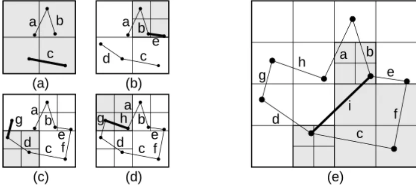
entries. The root node has at least two entries unless it is a leaf node.

h a b e f i c d g

Figure 1: Example collection of line segments embedded in a 44 grid.

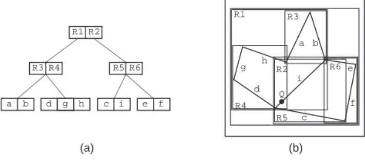
For example, consider the collection of line segments given in Figure 1 shown embedded in a 44 grid. Let

M

= 3 and

m

= 2. One possible r-tree for this collection is given in

Figure 2a. Figure 2b shows the spatial extent of the bounding rectangles of the nodes in Figure 2a, with broken lines denoting the rectangles corresponding to the subtrees rooted at the non-leaf nodes. Note that the r-tree is not unique. Its structure depends heavily

on the order in which the individual line segments were inserted into (and possibly deleted from) the tree.

R3 R1 R4 R5 R6 R2 R1 R2 R3 R4 R5 R6 a b d g h c i e f a b c d e f g h i Q (a) (b)

Figure 2: (a) R-tree for the collection of line segments in Figure 1, and (b) the spatial

extents of the bounding rectangles.

The drawback of these methods is that they do not result in a disjoint decomposition of space. The problem is that an object is only associated with one bounding rectangle (e.g., line segment iin Figure2 is associated with rectangle R5, yet it passes throughR1, R2,R4,

and R5). In the worst case, this means that when we wish to determine which object is

associated with a particular point (e.g., the containing rectangle in a rectangle database, or an intersecting line in a line segment database) in the two-dimensional space from which the objects are drawn, we may have to search the entire database.

For example, suppose we wish to determine the identity of the line segment in the collection of line segments given in Figure 2 that passes through pointQ. Since Qcan be in

either ofR1orR2, we must search both of their subtrees. Searching R1rst, we nd thatQ

could only be contained inR4. SearchingR4does not lead to the line segment that contains Qeven thoughQis in a portion of bounding rectangleR4that is inR1. Thus, we must search

R2and we nd thatQ can only be contained inR5. SearchingR5results in locating i, the

desired line segment.

The other approaches are based on a decomposition of space into disjoint cells, which are mapped into buckets. Their common property is that the objects are decomposed into disjoint subobjects such that each of the subobjects is associated with a dierent cell. They dier in the degree of regularity imposed by their underlying decomposition rules and by the way in which the cells are aggregated. The price paid for the disjointness is that in order to determine the area covered by a particular object, we have to retrieve all the cells that it occupies. This price is also paid when we want to delete an object. Fortunately, deletion is not so common in these databases. A related drawback is that when we wish to determine all the objects that occur in a particular region we often retrieve many of the objects more than once. This is particularly problematic when the result of the operation serves as input to another operation via composition of functions. For example, suppose we wish to compute the perimeter of all the objects in a given region. Clearly, each object's perimeter should only be computed once. Eliminating the duplicates is a serious issue (see [Aref and Samet 1992] for a discussion of how to deal with this problem in a database of line segments).

The rst method based on disjointness partitions the objects into arbitrary disjoint subobjects and then groups the subobjects in another structure such as a b-tree. The

partition and the subsequent groupings are such that the bounding rectangles are disjoint at each level of the structure. The r

+-tree [Sellis et al. 1987] and the cell tree [Gunther

1988] are examples of this approach. They dier in the data with which they deal. The

r

+-tree deals with collections of objects that are bounded by rectangles, while the cell tree

deals with convex polyhedra. Ther

+-tree is an extension of the

k-d-b-tree [Robinson 1981]. Ther

+-tree is motivated

by a desire to avoid overlap among the bounding rectangles. Each object is associated with all the bounding rectangles that it intersects. All bounding rectangles in the tree (with the exception of the bounding rectangles for the objects at the leaf nodes) are non-overlapping

2. The result is that there may be several paths starting at the root to the same object.

This may lead to an increase in the height of the tree. However, retrieval time is sped up.

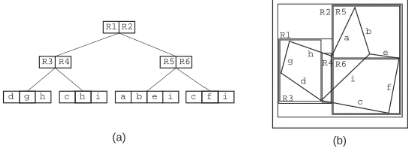
R5 R1 R3 R2 R6 R4 R1 R2 R3 R4 R5 R6 h i c a b c d e f g h i g h d a b e i c f i (a) _(b) Figure 3: (a) R

+-tree for the collection of line segments in Figure 1 and (b) the spatial

extents of the bounding rectangles.

Figure 3 is an example of one possible r

+-tree for the collection of line segments in 2

From a theoretical viewpoint, the bounding rectangles for the objects at the leaf nodes should also be disjoint. However, this may be impossible (e.g., when the objects are line segments where many line segments intersect at a point).

b-tree performance guarantees are not valid (i.e., pages are not guaranteed to be

m=M

full)

unless we are willing to perform very complicated record insertion and deletion procedures. Notice that line segments c and h appear in two dierent nodes, while line segment i

appears in three dierent nodes. Of course, other variants are possible since ther

+-tree is

not unique.

Methods such as ther

+-tree and the cell tree (as well as the r

-tree [Beckmann et al.

1990]) have the drawback that the decomposition is data-dependent. This means that it is dicult to perform tasks that require composition of dierent operations and data sets (e.g., set-theoretic operations such as overlay). In contrast, the remaining two methods, while also yielding a disjoint decomposition, have a greater degree of data-independence. They are based on a regular decomposition. The space can be decomposed either into blocks of uniform size (e.g., the uniform grid [Franklin 1984]) or adapt the decomposition to the distribution of the data (e.g., a quadtree-based approach such as [Samet and Webber 1985]). In the former case, all the blocks are of the same size (e.g., the 44 grid in Figure 1).

In the latter case, the widths of the blocks are restricted to be powers of two, and their positions are also restricted.

The uniform grid is ideal for uniformly distributed data, while quadtree-based ap-proaches are suited for arbitrarily distributed data. In the case of uniformly distributed data, quadtree-based approaches degenerate to a uniform grid, albeit they have a higher overhead. Both the uniform grid and the quadtree-based approaches lend themselves to set-theoretic operations and thus they are ideal for tasks which require the composition of dierent operations and data sets. In general, since spatial data is not usually uni-formly distributed, the quadtree-based regular decomposition approach is more exible. The drawback of quadtree-like methods is their sensitivity to positioning in the sense that the placement of the objects relative to the decomposition lines of the space in which they are embedded eects their storage costs and the amount of decomposition that takes place. This is overcome to a large extent by using a bucketing adaptation that decomposes a block only if it contains more than

n

objects.

All of the spatial occupancy methods discussed above are characterized as employing spatial indexing because with each block the only information that is stored is whether or not the block is occupied by the object or part of the object. This information is usually in the form of a pointer to a descriptor of the object. For example, in the case of a collection of line segments in the uniform grid of Figure 1, the shaded block only records the fact that a line segment crosses it or passes through it. The part of the line segment that passes through the block (or terminates within it) is termed a q-edge. Each q-edge in the block

is represented by a pointer to a record containing the endpoints of the line segment of which the q-edge is a part [Nelson and Samet 1986]. This pointer is really nothing more than a spatial index and hence the use of this term to characterize this approach. Thus no information is associated with the shaded block as to what part of the line (i.e., q-edge) crosses it. This information can be obtained by clipping [Foley et al. 1990] the original line segment to the block. This is important for often the precision necessary to compute these intersection points is not available.

A region can be represented either by its interior or by its boundary. In this section we focus on the representations of regions by their interior, while the use of a boundary is discussed in Section 6 in the context of collections of line segments as found, for example, in polygonal maps. The most common region representation is the image array. In this case, we have a collection of picture elements (termed pixels). Since the number of elements in the array can be quite large, there is interest in reducing its size by aggregating similar (i.e., homogeneous or equal-valued) pixels. There are two basic approaches. The rst approach breaks up the array into 1

m

blocks [Rutovitz 1968]. This is a row representation and

is known as a runlength code. A more general approach treats the region as a union of maximal square blocks (or blocks of any other desired shape) that may possibly overlap. Usually the blocks are specied by their centers and radii. This representation is called the medial axis transformation (MAT)[Blum 1967].

When the maximal blocks are required to be disjoint, to have standard sizes (squares whose sides are powers of two), and to be at standard locations (as a result of a halving process in both the

x

and

y

directions), the result is known as a region quadtree [Klinger 1971]. It is based on the successive subdivision of the image array into four equal-size quadrants. If the array does not consist entirely of 1s or entirely of 0s (i.e., the region does not cover the entire array), it is then subdivided into quadrants, subquadrants, etc., until blocks are obtained (possibly 11 blocks) that consist entirely of 1s or entirely of 0s. Thus,

the region quadtree can be characterized as a variable resolution data structure.

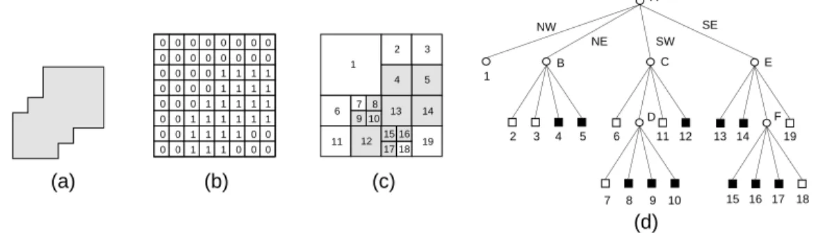
As an example of the region quadtree, consider the region shown in Figure 4a which is represented by the 23

2

3 binary array in Figure 4b. Observe that the 1s correspond to

pixels that are in the region and the 0s correspond to pixels that are outside the region. The resulting blocks for the array of Figure 4b are shown in Figure 4c. This process is represented by a tree of degree 4.

0 0 0 0 0 0 0 0 0 0 0 0 0 0 0 0 0 0 0 0 0 0 0 0 0 0 0 0 0 0 0 0 0 0 0 0 0 0 1 1 1 1 1 1 1 1 1 1 1 1 1 1 1 1 1 1 1 1 1 1 1 1 1 1 1 2 3 4 5 6 7 8 9 10 13 11 12 14 15 16 17 18 19 A NW NE SW SE 1 2 3 4 5 6 11 12 13 14 19 7 8 9 10 15 16 17 18 B C D F E (a) (b) (c) (d)

Figure4: (a) Sample region, (b) its binary array representation, (c) its maximal blocks with

the blocks in the region being shaded, and (d) the corresponding quadtree.

In the tree representation, the root node corresponds to the entire array. Each son of a node represents a quadrant (labeled in order nw, ne, sw, se of the region represented

by that node. The leaf nodes of the tree correspond to those blocks for which no further subdivision is necessary. A leaf node is said to be black orwhite, depending on whether

its corresponding block is entirely inside or entirely outside of the represented region. All non-leaf nodes are said to be . The quadtree representation for Figure 4c is shown in

map, simply merge all wheat growing regions, and likewise for corn, rice, etc. [Samet et al. 1984].

The term quadtree is often used in a more general senses to describe a class of hierarchical data structures whose common property is that they are based on the principle of recursive decomposition of space. They can be dierentiated on the following bases:

1. the type of data that they are used to represent, 2. the principle guiding the decomposition process, and 3. the resolution (variable or not).

Currently, they are used for points, rectangles, regions, curves, surfaces, and volumes (see the remaining sections for further details on the adaptation of the quadtree to them). The decomposition may be into equal parts on each level (termed a regular decomposition), or it may be governed by the input. The resolution of the decomposition (i.e., the number of times that the decomposition process is applied) may be xed beforehand or it may be governed by properties of the input data.

Unfortunately, the term quadtree has taken on more than one meaning. The region quadtree, as shown above, is a partition of space into a set of squares whose sides are all a power of two long. A similar partition of space into rectangular quadrants is termed a point quadtree [Finkel and Bentley 1974]. It is an adaptation of the binary search tree to two dimensions (which can be easily extended to an arbitrary number of dimensions). It is primarily used to represent multidimensional point data where the rectangular regions need not be square. The quadtree is also often confused with the pyramid [Tanimoto and Pavlidis 1975]. The pyramid is a multiresolution representation which is an exponentially tapering stack of arrays, each one-quarter the size of the previous array. In contrast, the region quadtree is a variable resolution data structure.

The distinction between a quadtree and a pyramid is important in the domain of spatial databases, and can be easily seen by considering the types of spatial queries. There are two principal types [Aref and Samet 1990]. The rst is location-based. In this case, we are searching for the nature of the feature associated with a particular location or in its proximity. For example, \what is the feature at location X?", \what is the nearest city to location X?", or \what is the nearest road to location X?" The second is feature-based. In this case, we are probing for the presence or absence of a feature, as well as seeking its actual location. For example, \does wheat grow anywhere in California?", \what crops grow in California?", or \where is wheat grown in California?"

Location-based queries are easy to answer with a quadtree representation as they involve descending the tree until nding the object. If a nearest neighbor is desired, then the search is continued in the neighborhood of the node containing the object. This search can also be achieved by unwinding the process used to access the node containing the object. On the other hand, feature-based queries are more dicult. The problem is that there is no indexing by features. The indexing is only based on spatial occupancy. The goal is to process the query without examining every location in space. The pyramid is useful for

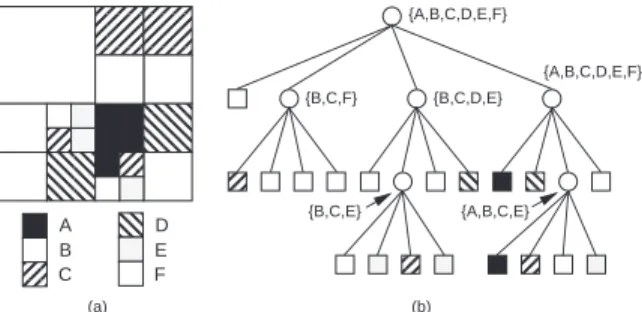
such queries since the nodes that are not at the maximum level of resolution (i.e., at the bottom level) contain summary information. Thus we could view these nodes as feature vectors which indicate whether or not a feature is present at a higher level of resolution. Therefore, by examining the root of the pyramid (i.e., the node that represents the entire image) we can quickly tell if a feature is present without having to examine every location. For example, consider the block decomposition of the non-binary image in Figure 5a. Its truncated pyramid is given in Figure 5b. The values of a nonleaf nodepin the truncated

pyramid indicate if the feature is present in the subtrees ofp. In the interest of saving space,

the pyramid is not shown in its entirety here.

AAAA AAAA AAAA AAAA AAA AAA AAA AA AA AA AAA AAA AAA AAA AAA AA AA AA AA AAA AAA AA AA AA AA AA A A AA AAAA A A AA AA AA AA A B C AA AA_D E AA AAF AA AA AA AA AA AA AA AA AAAA AAAA AA AA AA AA AA AA AA AA AA AA AA {A,B,C,D,E,F} {B,C,F} {B,C,D,E} {A,B,C,D,E,F} {B,C,E} {A,B,C,E} (a) (b)

Figure 5: (a) Sample non-binary image, and (b) its corresponding truncated pyramid.

Quadtree-like data structures can also be used to represent images in three dimensions and higher. The octree [Hunter 1978; Meagher 1982] data structure is the three-dimensional analog of the quadtree. It is constructed in the following manner. We start with an image in the form of a cubical volume and recursively subdivide it into eight congruent disjoint cubes (called octants) until blocks are obtained of a uniform color or a predetermined level of decomposition is reached. Figure 6a is an example of a simple three-dimensional object whose raster octree block decomposition is given in Figure 6b and whose tree representation is given in Figure 6c. 1 2 3 4 13 14 15 12 11 10 9 8 7 6 5 B A 14 15 4 9 10 6 1 2 13 12 11 5 (a) (b) (c)

Figure6: (a) Example three-dimensional object; (b) its octree block decomposition; and (c)

its tree representation.

The quadtree is particularly useful for performing set operations as they form the basis of most complicated queries. For example, to \nd the names of the roads that pass through the University of Maryland region," we will need to intersect a region map with a line map. For a binary image, set-theoretic operations such as union and intersection are quite simple to implement [Hunter and Steiglitz 1979].

In particular, the intersection of two quadtrees yields a black node only when the

corresponding regions in both quadtrees are black. This operation is performed by

aregray, then their sons are recursively processed and a check is made for the mergibility

of white leaf nodes. The worst-case execution time of this algorithm is proportional to

the sum of the number of nodes in the two input quadtrees, although it is possible for the intersection algorithm to visit fewer nodes than the sum of the nodes in the two input quadtrees.

Performing the set operations on an image represented by a region quadtree is much more ecient than when the image is represented by a boundary representation (e.g., vectors) as it makes use of global data. In particular, to be ecient, a vector-based solution must sort the boundaries of the region with respect to the space which they occupy, while in the case of a region quadtree, the regions are already sorted.

One of the motivations for the development of hierarchical data structures such as the quadtree is a desire to save space. The original formulation of the quadtree encodes it as a tree structure that uses pointers. This requires additional overhead to encode the internal nodes of the tree. In order to further reduce the space requirements, two other approaches have been proposed. The rst treats the image as a collection of leaf nodes where each leaf is encoded by a pair of numbers. The rst is a base 4 number termed a locational code, corresponding to a sequence of directional codes that locate the leaf along a path from the root of the quadtree (e.g., [Gargantini 1982]). It is analogous to taking the binary representation of thexandy coordinates of a designated pixel in the block (e.g., the one at

the lower left corner) and interleaving them (i.e., alternating the bits for each coordinate). The second number indicates the depth at which the leaf node is found (or alternatively its size).

The second, termed a DF-expression, represents the image in the form of a traversal of the nodes of its quadtree [Kawaguchi and Endo 1980]. It is very compact as each node type can be encoded with two bits. However, it is not easy to use when random access to nodes is desired. For a static collection of nodes, an ecient implementation of the pointer-based rep-resentation is often more economical spacewise than a locational code reprep-resentation [Samet and Webber 1989]. This is especially true for images of higher dimension.

Nevertheless, depending on the particular implementation of the quadtree we may not necessarily save space (e.g., in many cases a binary array representation may still be more economical than a quadtree). However, the eects of the underlying hierarchical aggregation on the execution time of the algorithms are more important. Most quadtree algorithms are simply preorder traversals of the quadtree and, thus, their execution time is generally a linear function of the number of nodes in the quadtree. A key to the analysis of the execution time of quadtree algorithms is the Quadtree Complexity Theorem [Hunter 1978] which states that the number of nodes in a quadtree region representation isO(p+q) for a

2q 2

q image with perimeter

pmeasured in pixel-widths. In all but the most pathological

cases (e.g., a small square of unit width centered in a large image), theqfactor is negligible

and thus the number of nodes isO(p).

The Quadtree Complexity Theorem holds for three-dimensional data [Meagher 1980] where perimeter is replaced by surface area, as well as for objects of higher dimensions d

for which it is proportional to the size of the (d,1)-dimensional interfaces between these