Spectral approximation of the IMSE criterion for
optimal designs in kernel-based interpolation models.
Bertrand Gauthier, Luc Pronzato
To cite this version:
Bertrand Gauthier, Luc Pronzato. Spectral approximation of the IMSE criterion for
opti-mal designs in kernel-based interpolation models.. SIAM/ASA Journal on Uncertainty
Quan-tification, 2014, 2, pp.805-825.
<
http://epubs.siam.org/doi/abs/10.1137/130928534
>
.
<
hal-00913466v4
>
HAL Id: hal-00913466
https://hal.archives-ouvertes.fr/hal-00913466v4
Submitted on 21 Nov 2014
HAL
is a multi-disciplinary open access
archive for the deposit and dissemination of
sci-entific research documents, whether they are
pub-lished or not.
The documents may come from
teaching and research institutions in France or
abroad, or from public or private research centers.
L’archive ouverte pluridisciplinaire
HAL, est
destin´
ee au d´
epˆ
ot et `
a la diffusion de documents
scientifiques de niveau recherche, publi´
es ou non,
´
emanant des ´
etablissements d’enseignement et de
recherche fran¸
cais ou ´
etrangers, des laboratoires
publics ou priv´
es.
SPECTRAL APPROXIMATION OF THE IMSE CRITERION FOR OPTIMAL DESIGNS
IN KERNEL-BASED INTERPOLATION MODELS
BERTRAND GAUTHIER† ∗ AND LUC PRONZATO‡ ∗
Abstract. We address the problem of computing IMSE-optimal designs for random field inter-polation models. A spectral representation of the IMSE criterion is obtained from the eigendecom-position of the integral operator defined by the covariance kernel of the random field and integration measure considered. The IMSE can then be approximated by spectral truncation and bounds on the error induced by this truncation are given. We show how the IMSE and truncated-IMSE can be easily computed when a quadrature rule is used to approximate the integrated MSE and the design space is restricted to a subset of quadrature points. Numerical experiments are carried out and indicate (i) that retaining a small number of eigenpairs (in regard to the quadrature size) is often sufficient to obtain good approximations of IMSE optimal quadrature-designs when optimizing the truncated criterion and (ii) that optimal quadrature-designs generally give efficient approximations of the true optimal designs for the quadrature approximation of the IMSE.
Key words. Random field model, interpolation, design of experiments, IMSE, integral operator, quadrature approximation.
AMS subject classifications. 62K99, 65C60, 62G08
1. Introduction. This work adresses the problem of designing experiments (i.e., of choosing sampling points) in the framework of kernel-based interpolation models (see for instance [RW06, Wah90]). The integrated mean-squared error (IMSE) cri-terion is a classical tool for evaluating the overall performance of interpolators (see for example [SWMW89]). For a fixed class of models and a given design size, it is therefore natural to try to choose sampling points such that the resulting interpola-tion minimizes the IMSE criterion among all possible samplings. One then speaks of IMSE-optimal design of experiments.
IMSE-optimal designs are generally considered as difficult to compute, see, e.g., [SWMW89, ABM12]. Indeed, the direct evaluation of the IMSE criterion is numer-ically expensive (it requires the computation of the integral of the mean-squared prediction error over the whole space) and its global optimization is often made dif-ficult due to the presence of many local minima (many evaluations of the criterion are thus required). The present work aims at investigating an alternative approach to make the computation of IMSE-optimal designs more tractable by reducing the computational cost of the criterion evaluation.
The choice of an IMSE criterion for learning a random field leads to the definition of an integral operator (see Section3and, e.g., [ST06]). The interest of such operators when dealing with kernel-based interpolation models has been discussed for instance in [CS02,LMK10,GB12], see also [SY66, DPZ13] for applications to optimal design for linear regression models with correlated errors. The main idea of the present work is to link the IMSE criterion with the spectral decomposition of its associated integral operator. We hence obtain a spectral representation of the IMSE criterion which can be approximated by spectral truncation, with guaranteed bounds on the error induced by truncation.
†[email protected] ‡[email protected]
∗CNRS, Laboratoire I3S - UMR 7271, Université de Nice-Sophia Antipolis/CNRS, France. 1
From a numerical point of view, the IMSE and truncated-IMSE criteria can be easily computed when a (pointwise) quadrature is used to approximate the integral of the MSE and the design construction is restricted to quadrature-designs (i.e., de-signs only composed of quadrature points, see Definition4.2). Numerical experiments indicate that retaining a small number of eigenpairs (in regard to the quadrature size) is often sufficient to obtain efficient approximation of IMSE-optimal quadrature-designs when optimizing the truncated criterion. They also indicate that optimal quadrature-designs in general give good approximations of the true optimal designs for the quadrature approximation of the IMSE, so that the restriction to quadrature points appears to have small impact (this restriction has sometimes no impact at all, see in particular Remark5.1).
We have tried to make the paper as self-contained as possible: the definitions of most concepts are reminded and most proofs are detailed (in the body of the paper or, for the sake of readability, in an appendix). We first describe a general setting in which the spectral representation of the IMSE is well-defined. We next focus on the classical IMSE optimal design problem (conditioning by a finite number of evaluations), with particular attention to the quadrature approximation case.
The paper is organized as follows. Section2 is devoted to the introduction of the general framework of conditioning Gaussian random fields. General results concerning the IMSE criterion and the associated integral operator are given in Section3, where the spectral representation of the IMSE criterion and its approximation by spectral truncation are detailed. The computation and the approximation of the IMSE crite-rion for designing experiments is considered in Section4. Numerical experiments are carried out in Section5. Section6concludes and gives some perspectives.
2. General framework and notations.
2.1. Random fields and involved Hilbert structures. LetX be a general set. We consider a real random field(Zx)x∈X indexed by X. We assume thatZ is centered, second-order, and defined on a probability space(Ω,F,P). For the sake of
simplicity, we also assume that Z is Gaussian (so that the optimal linear prediction is the optimal prediction). In what follows,Z will refer to the random field(Zx)x∈X.
We denote byL2(Ω,
P)the Hilbert space of second-order, real random variables
(r.v.) on(Ω,F,P), where we identify random variables that are equalP-almost surely.
The inner product between two r.v. U andV ofL2(Ω,
P)is denoted byE(U V).
Let K :X × X → R be the covariance kernel of the random fieldZ. Since, by
assumption, for allxandy∈ X,E(Zx) =E(Zy) = 0, we have
E(ZxZy) =K(x, y).
We denote by H the Gaussian Hilbert space generated by Z; H is the closed linear subspace ofL2(Ω,
P)spanned by the r.v. Zx,x∈ X, i.e.,
H= span{Zx, x∈ X } L2(Ω,
P)
.
The linear spaceHis endowed with the Hilbert structure involved by L2(Ω,
P). For
the sake of simplicity, we assume thatH is separable (see RemarkB.1).
In parallel, we denote byHthe reproducing kernel Hilbert space (RKHS, see for instance [BT04]) of real-valued functions onX associated with the kernelK(·,·). We use the classical notation,Kx(·) =K(x,·), forx∈ X (andKx∈ H). We remind that His characterized by the representation property,
with(·|·)H the inner product ofH. Also, if {hj, j∈J}is an orthonormal basis ofH,
we have
∀xandy∈ X, K(x, y) =X j∈J
hj(x)hj(y). (2.2)
The two Hilbert spacesHandHare isometric thanks to the relation, for allxand
y ∈ X, (Kx|Ky)H =K(x, y) =E(ZxZy). We denote this isometry by I :H → H,
withI(Kx) =Zx.
2.2. Conditioning. Let HD be a closed linear subspace of the Hilbert space
H. We consider the orthogonal projection PHD of H ontoHD. For x∈ X, the r.v.
PHD[Zx] is called the conditional mean of the r.v. Zx relatively to HD. If HD is
spanned by the r.v. ζj,j∈J, withJ a general index set, the notation
PHD[Zx] =E(Zx|ζj, j∈J)
is often used. The covariance of the random field (Zx−PHD[Zx])x∈X is called the
conditional covariance of Z relatively toHD. We shall pay particular attention to
subspaces of the evaluation-type, i.e.,
Hev= span{Zx1,· · ·, Zxn}, (2.3)
withn∈N∗ (the set of all positive integers) andx1,· · ·, xn ∈ X, see Section4. Remark 2.1. By isometry, a conditioning problem in the Gaussian Hilbert spaceH
is associated with an optimal interpolation problem in the RKHSH. To the subspace
HDofHcorresponds a subspaceHDofHand one can define the orthogonal projection
PHD ofHontoHD, etc. /
3. IMSE criterion and associated integral operator.
3.1. IMSE criterion and working hypotheses. From now on we suppose thatX is a measurable space and we consider aσ-finite measure µonX. We denote byL2(X, µ)the (not necessarily separable) Hilbert space of square integrable (with
respect toµ) real-valued functions onX. Notice that elements ofL2(X, µ)are in fact
equivalent classes of µ-almost everywhere equal functions; however, when it will not be source of confusion, we shall assimilate elements ofL2(X, µ)with functions on X.
We make the following assumptions throughout the rest of the paper: C-i. anyh∈ His a measurable function,
C-ii. the kernelK:X × X →Ris measurable (for the productσ-algebra),
C-iii. τ=
Z
X
K(x, x)dµ(x)<+∞.
For a given closed linear subspace HD of H, the integrated mean-squared error
criterion associated with HD (IMSE, or when necessary µ-IMSE, to explicitly refer
to the measure µ) is the integral of the conditional variance of Z relatively to HD;
more precisely, IMSE(HD) = Z XE h (Zx−PHD[Zx]) 2i dµ(x) = Z X n K(x, x)−E(PHD[Zx]) 2odµ(x). 3
Under the assumptions above, IMSE(HD) is well-defined for any closed linear sub-spaceHD ofH (see RemarkB.2) and we have
IMSE(HD) =τ−CI(HD), withCI(HD) = Z XE (PHD[Zx]) 2dµ(x). (3.1)
Sinceτdoes not depend onHD, minimizing the IMSE amounts to maximizeCI(HD),
and we haveCI({0}) = 06CI(HD)6CI(H) =τ.
3.2. Integral operator defined by the IMSE. Under conditions C-i, C-ii and C-iii, the introduction of an IMSE criterion for the learning of a random fieldZ
defines an integral operatorTµonL2(X, µ). We first recall the following lemma; the
proof is given in AppendixA.
Lemma 3.1. Under conditions C-i and C-iii, the RKHS His continuously included intoL2(
X, µ), that is, for allh∈ H,h∈L2(
X, µ)and khk2L2 6τkhk
2
H. (3.2)
From Lemma3.1, we know thatKx∈L2(X, µ)for allx∈ X and we can therefore
define, without ambiguity,
∀f ∈L2(X, µ), ∀x∈ X, Tµ[f] (x) = Kx fL2 = Z X f(t)K(x, t)dµ(t).
Let us now recall some of the main properties of the operator Tµ (the proof of
Lemma3.2is given in AppendixA).
Lemma 3.2. Under C-i, C-ii and C-iii, we have K(·,·) ∈ L2(
X × X, µ⊗µ) and the operator Tµ is a compact (Hilbert-Schmidt), self-adjoint and positive operator on
L2( X, µ).
From Lemma3.2and the spectral theorem for compact self-adjoint operators on Hilbert spaces (see for instance [Sch79]), Tµ is diagonalizable and its eigenfunctions
form a complete orthogonal system. We denote by λi >0 its eigenvalues (repeated
according to their geometric multiplicity) and byφei∈L2(X, µ)the associated
eigen-functions, with i ∈ I, a general index set. We classically choose the eigenfunctions
eφi, i∈I so that they form an orthonormal basis of L2(X, µ). We also denote by
λk, k∈I+ the set (at most countable) of all strictly positive eigenvalues ofTµ, that
isλk>0for allk∈I+.
Proposition 3.1. Let H0 be the linear subspace ofHdefined by H0=
n
h0∈ H,kh0k2L2 = 0
o
.
Denote byHµ the orthogonal ofH0 inH(i.e., Hµ =H⊥0H) and, fork∈I+, consider the functions φk given by
∀x∈ X, φk(x) = 1 λk Z X e φk(t)K(x, t)dµ(t) = 1 λk e φk|KxL2 = 1 λkTµ eφk(x). (3.3) ThenH0 is closed inHand√λkφk, k∈I+ forms an orthonormal basis ofHµ for the Hilbert structure ofH.
Remark 3.1. We have φk
L2(X,µ)
= φek (or more precisely, φk belongs to the
equiva-lent class φek). However, as elements of L2(X, µ), theφek are only definedµ-almost
everywhere whereas theφk are defined on the whole setX.
For allf ∈L2(X, µ)andh∈ H, we have (see the proof of Proposition3.1)
Tµ[f]∈ Hµ and (h|f)L2 = (h|Tµ[f])H.
Therefore, the functionsφk∈ Hsatisfy the following property: ∀h∈ H, ∀k∈I+, (h|φk)H= 1 λk hTµ[φek]H= 1 λk heφkL2
and in particular, for k ∈ I+ and x ∈ X, φk
KxL2 = λk φk
KxH = λkφk(x).
Notice thatτ =Pk∈I+λk, see C-iii. / 3.3. Spectral representation of the IMSE. For k ∈ I+, we introduce the
r.v. ξk = I √λkφk ∈ H, where I is the isometry between H and H defined in
Section2.1, so that the ξk,k∈I+, are orthonormal inH. Following Proposition3.1,
we denote byHµ the closed linear subspace ofHspanned by the r.v. ξk,k∈I+and
byH0 its orthogonal, so that we have the orthogonal decomposition
H=Hµ ⊥
+H0. (3.4)
Proposition 3.2. Let HD be a closed linear subspace ofH, we have
CI(HD) =CI(HD∩Hµ), whereCI is defined in equation (3.1).
Proof. From (3.4), we have the orthogonal decompositionHD =HµD+H0D, where
HµD =Hµ∩HDandH0D=H0∩HD. The orthogonal projection ofH ontoHDis
then given byPHD =PHµD+PH0D.
For allx∈ X, the r.v. PHµD[Zx]andPH0D[Zx]are orthogonal, hence
E(PHD[Zx]) 2= E(PHµD[Zx]) 2+ E(PH0D[Zx]) 2,
so that CI(HD) = CI(HD∩Hµ) +CI(HD∩H0). To conclude, we consider an
orthonormal basis{gj, j∈J}of the RKHSH0D. From (2.2), we have
CI(H0D) = Z X K0D(x, x)dµ(x) = X j∈J Z X g2j(x)dµ(x) = 0,
since gj ∈ H0 for all j ∈ J, where K0D(·,·) is the reproducing kernel of H0D (the
interchange between the sum and the integral is justified by Tonelli’s theorem).
Proposition 3.3(Spectral representation of the IMSE criterion). LetHDbe a closed linear subspace of H and let {ηj, j ∈ J} be an orthonormal basis of HD. Then, we have CI(HD) = X k∈I+ X j∈J α2j,kλk, (3.5)
with, forj∈J andk∈I+,αj,k=E(ηjξk).
Proof. From Proposition3.1,{ξk, k∈I+}forms an orthonormal basis ofHµ, so that ∀j∈J, PHµ[ηj] =
X
k∈I+
αj,kξk. (3.6)
For any r.v. U ∈H, we have
PHD[U] = X j∈J E(ηjU)ηj andE h (PHD[U]) 2i =X j∈J E(ηjU) 2 . (3.7) Combining relations (3.7) with Proposition3.2, we obtain
CI(HD) =CI(HD∩Hµ) = Z XE h PHD PHµ[Zx] 2i dµ(x) = Z X X j∈J E ηjPHµ[Zx] 2 dµ(x). (3.8) For allx∈ X, we havePHµ[Zx] =
P k∈I+ξkE(ξkZx) = P k∈I+ξk √ λkφk(x). Injecting
this expansion in (3.8) and using (3.6), we obtain
CI(HD) = X j∈J Z X X k∈I+ αj,k p λkφk(x) 2 dµ(x) = X k∈I+ X j∈J α2 j,kλk,
which completes the proof.
We now recall the following well-known result (Proposition3.4), which shows the optimal character of the r.v. ξk,k∈I+, in terms of IMSE.
Proposition 3.4. For a fixed n ∈ N∗, consider H∗n = span{ξ1,· · · , ξn}, where
ξ1,· · ·, ξn are associated with the n largest eigenvalues of Tµ, denoted respectively by λ1>· · ·>λn. Then H∗n minimizes the IMSE criterion among all subspaces Hn of Hwith dimension nandCI(H∗n) =
Pn k=1λk.
Notice thatH∗n is not necessarily unique, depending of the multiplicity ofλn. Proof. LetHnbe a closed linear subspace ofHµ with dimensionn(the restriction to
subsets ofHµis justified from Proposition3.2) and let{η1,· · ·, ηn}be an orthonormal
basis ofHn. From Proposition3.3, since {ξ1,· · ·, ξn}forms an orthonormal basis of
H∗
n, we haveCI(H∗n) =P n k=1λk.
For any i and j ∈ {1,· · ·, n}, we have Pk∈
I+αi,kαj,k =δij (Kronecker delta).
Fork∈I+, letak∈Rn be the column vector given byak= (α1,k, . . . , αn,k)T, so that
Pn
j=1α2j,k=aTkak, where aTk stands for the transpose of the vectorak. We also have
P
k∈I+aka
T
k = Idn×n (then×nidentity matrix). Therefore, forl∈I+,
aTl X k∈I+ akaTk al=aTlal= aTl al 2 +X k6=l aTlak 2 ,
which proves that
∀k∈I+, n X j=1 α2j,k61. (3.9) For j ∈ {1,· · ·, n}, we have Pk∈I +α 2 j,k = 1 and therefore P k∈I+ Pn j=1α2j,k = n.
Sinceλ1,· · ·, λn are the largest eigenvalues ofTµ, we deduce from this equality
com-bined with (3.9) that Pnj=1λj >Pk∈I+
Pn
j=1α2j,kλk, i.e.,CI(H∗n)>CI(Hn), which
3.4. Approximation by truncation. The spectral representation of the IMSE criterion can be approximated by truncation.
Definition 3.1. Let HD be a closed linear subspace of H with orthonormal basis {ηj, j ∈ J} and consider the notation of Proposition 3.3. For a subset Itrc of I+, the (spectral) truncated-IMSE criterion associated with the subspace HD is given by IMSEtrc(HD) =τtrc−CItrc(HD), with CItrc(HD) = X k∈Itrc X j∈J α2j,kλk (3.10) and whereτtrc=Pk∈Itrcλk.
Remark 3.2. We have chosen to use τtrc in Definition 3.1 since we interpret the
truncated-IMSE criterion as the IMSE when only a subset of the eigenvalues is taken
into account. /
Proposition 3.5(Error induced by truncation). For any closed linear subspaceHD of Hand for any truncation set Itrc⊂I+, we have,
CItrc(HD)6CI(HD)6CItrc(HD) +
X
k6∈Itrc
λk, so that Pk6∈
Itrcλk gives an upper bound on the error induced by truncation.
Proof. Consider the notations of Proposition 3.3 and the spectral expansions of CI
and CItrc given in (3.5) and (3.10). The left-hand side inequality follows from the
positivity of all the α2
j,kλk. For the right-hand side inequality, we just have to note
that, similarly to (3.9), for allk∈I+ we havePj∈Jα2j,k61.
The accuracy of the approximation by truncation is usually quantified through the spectral ratio
Rtrc= τtrc τ = P k∈Itrcλk P k∈I+λk .
In practice, we shall consider truncations that only use the ntrc ∈N∗ largest
eigen-values of the spectrum and the number ntrc of elements of Itrc will be called the truncation level.
Remark 3.3. LetHnbe a closed linear subspace ofHµwith dimensionnand consider
the framework of the proof of Proposition 3.4. For a truncation setItrc ⊂I+, since
P
k∈I+
Pn
j=1α2j,k = n, we also have the following bound for the error induced by
truncation: CI(Hn)−CItrc(Hn) = X k6∈Itrc n X j=1 α2j,kλk6 n− X k∈Itrc n X j=1 α2j,k max k6∈Itrc (λk). (3.11) Notice that contrary to Proposition 3.5, the bound (3.11) depends on the subspace
Hn considered. /
4. IMSE and design of experiments.
4.1. Classical approach. Denote byzthe (column) random vector
z= (Zx1,· · ·, Zxn) T
,
wherex1,· · ·, xn ∈ X andn∈N∗. We thus consider the design{x1,· · · , xn}and the
associated subspaceHev ofHdefined by equation (2.3).
Definition 4.1. For a fixedn∈N∗, a set{x1,· · ·, xn} ofnpoints ofX is ann-point IMSE-optimal design (for the learning ofZ) ifHev= span{Zx1,· · · , Zxn}minimizes the IMSE criterion among all subspaces of H based on nevaluations of the random fieldZ.
Letkbe the (column) vector of functions with componentsKxi,16i6n, that
is, forx∈ X,k(x) = Kx1(x),· · ·, Kxn(x)
T
. Also, letKbe the covariance matrix of
z. For the sake of simplicity, we assume that the random fieldZand{x1,· · ·, xn}are
such thatKis invertible (a generalized inverse ofKcan be used otherwise in order to express the orthogonal projection PHev). The simple kriging predictor is then given
by ∀x∈ X, PHev[Zx] =E Zx Zx1,· · ·, Zxn =kT(x)K−1z,
and the corresponding IMSE isIMSE(Hev) =τ−CI(Hev), where
CI(Hev) =
Z
X
kT(x)K−1k(x)dµ(x). (4.1)
In this form, from a numerical point of view the computation of the IMSE criterion for the design{x1,· · ·, xn}requires the inversion of the matrixKand the integration
of the functionx7→kT(x)K−1k(x).
4.2. Spectral representation and truncation of the IMSE. For a design of experiments{x1,· · ·, xn}, we introduce the matrixFwith entries
Fi,k=λkφk(xi) =
p
λkE(ξkZxi), with16i6nandk∈I+. (4.2)
Hence,Fhasnrows andcard (I+)columns, withcard (I+)6+∞. Proposition 4.1. Let Hev= span{Zx1,· · · , Zxn}, then
CI(Hev) = X k∈I+ h (F·,k)TK−1(F·,k) i = trace FTK−1F, (4.3)
where F·,k is thek-th column of the matrix F. If we consider a truncation based on a subsetItrc⊂I+, then CItrc(Hev) = X k∈Itrc h (F·,k)TK−1(F ·,k) i = trace (F·,Itrc) TK−1(F ·,Itrc) , (4.4)
whereF·,Itrc is the matrix with columns given by F·,k,k∈Itrc.
Proof. Expression (4.3) is a direct consequence of Proposition3.3applied to the eval-uation case. Indeed, let K =CCT be the Cholesky decomposition of K, then the
components of the random vector (η1,· · ·, ηn)T =C−1zform an orthonormal basis
of Hev. Consider the diagonal matrix Λ = diag (λk, k∈I+). With (4.2) and the
notations introduced in the proof of Proposition 3.4, we have ak = C−1FΛ−
1 2
·,k,
so that λkaTkak = λkPnj=1α2j,k = (F·,k)TK−1(F·,k). We hence obtain CI(Hev) =
P
k∈I+
h
(F·,k)TK−1(F·,k)
i
, which gives (4.3). The proof is similar for (4.4).
Expressions (4.3) and (4.4) indicate that once the functions λkφk(·)are known, IMSE(Hev) and IMSEtrc(Hev) can be obtained without explicitly integrating the mean-squared prediction error.
The two expressions (4.3) and (4.4) involve summations overI+ or Itrc. In
ad-dition, the computation of φk(x) for a general x ∈ X from the eigenpair {λk,φek}
using expression (3.3) requires the computation of an integral, which seriously limits the interest of (4.3) and (4.4). On the other hand, suppose that X is a topological space (endowed with its Borelσ-algebra) and that the RKHSHconsists of continuous functions onsupp(µ)⊂ X (the support ofµ). Then, by choosing a representer for the equivalent classφekwhich is continuous onsupp(µ)(and denotingφekthis representer),
we haveφek(x) =φk(x)for all x∈supp(µ). It is thus possible to evaluate and
opti-mize the IMSE criterion onsupp(µ)by using only the spectral decomposition of the operatorTµ. This will be of particular interest when the measureµis discrete, which
is the case for instance when a quadrature rule is used to approximate the integral of the MSE. This situation is detailed in Section4.4.
4.3. Alternative expressions for the IMSE and truncated-IMSE. Start-ing from (4.1) and using the property of the trace operator, we obtain
CI(Hev) = traceK−1
Z
X
k(x)kT(x)dµ(x)= trace K−1Σ, (4.5)
whereΣ=RXk(x)kT(x)dµ(x)is then
×nsymmetric matrix with i, jentry
Z
X
Kxi(x)Kxj(x)dµ(x) =Tµ[Kxj](xi) =Tµ[Kxi](xj).
We can then introduce the kernelΣ(·,·)onX × X, with
∀sandt∈ X, Σ(s, t) =
Z
X
Ks(x)Kt(x)dµ(x),
so thatΣ hasi, j entryΣ(xi, xj). In the same way, for the truncated criterion (4.4)
with truncation setItrc, we get
CItrc(Hev) = trace K −1Σ
trc, (4.6)
whereΣtrc=F·,Itrc(F·,Itrc)
T, so that thei, j entry ofΣ
trcisΣtrc(xi, xj), with ∀sandt∈ X, Σtrc(s, t) = X
k∈Itrc
λ2kφk(s)φk(t).
In a design optimization perspective, anticipating a large number of criterion evaluations to be performed, expressions (4.5) and (4.6) are of particular interest when the design spaceX0 is restricted to a finite subset of points inX. Indeed, one can then compute and store, preliminary to design optimization, the values of the (symmetric) kernelsΣ(·,·)and Σtrc(·,·)for all pairs of points belonging toX0. The computational cost of one evaluation of the IMSE or truncated-IMSE then mainly corresponds to the cost for inverting the matrixK(see also Remark4.1below). Such a situation is considered in Section4.4.2, where the design space is restricted to the set of quadrature points used to approximate the integrated MSE.
Remark 4.1. LetAbe al×mmatrix and letBbe am×lmatrix, withlandm∈N∗.
It is computationally advantageous to calculatetrace(AB)as sum A∗BT, with∗
standing for the Hadamard matrix product (i.e., element by element) and sum(·)
indicating the sum of all the elements of the matrix considered, thereby avoiding the computation of the off-diagonal elements of the productAB. /
4.4. Quadrature approximation. Consider the situation where a (pointwise) quadrature rule is used in order to approximate integrals overX with respect to µ.
4.4.1. Notations. For a real-valued function f on X, integrable with respect to µ, we consider the following approximation: R
Xf(s)dµ(s) ≈
PNq
j=1ωjf(sj), with
ωj >0, sj∈ X andNq ∈N∗. This situation thus corresponds to a particular case of
the general problem studied in Section3, where the measureµonX is approximated by the discrete measure
b µ= Nq X j=1 ωjδsj, (4.7)
withδsj the Dirac measure (evaluation functional) atsj. We thus obtain an
approx-imation Tµb of the integral operator Tµ (Nyström method, see for instance [Hac95,
Kre99]), ∀x∈ X, Tµ[bf](x) = Nq X j=1 ωjK(x, sj)f(sj).
Throughout the rest of the paper, the hat symbol indicates that the corresponding object is associated with the quadrature approximation µb. For instance, λbk refers
to an eigenvalue of Tµb, whereas λk refers to an eigenvalue of Tµ, etc. The results
contained in this section can be deduced from those of Section 3.2. However, due to the great importance of quadrature approximations in our study, some details are given below.
We introduce the twoNq×Nq matricesW= diag ω1,· · · , ωNq
andQwithi, j
termQi,j=K(si, sj), for16i, j 6Nq. The matrix Wis thus the diagonal matrix
of quadrature weights andQis the covariance matrix for the quadrature points. We can identify the Hilbert space L2(X,µb)with the space
RNq endowed with the inner
product (·|·)W, where for x andy ∈ RNq, (x|y)W = xTWy. To f ∈L2(X,µb), we
associate the vector f = f(s1),· · ·, f(sNq)
T
∈ RNq (i.e., f is the column vector
with components the values off at the quadrature points) and the operatorTbµthen
corresponds to the matrixQW. In matrix notation, we have
∀x∈ X, Tµb[f] (x) =qT(x)Wf,
with, for allx∈ X, q(x) = Ks1(x),· · · , KsNq(x)
T
.
For the sake of simplicity, we assume that Qis nonsingular (if Qwere singular, thenQWwould have some zero eigenvalues which can be ignored, see Section3.3). We denote bybλ1>· · ·>bλNq >0the eigenvalues of the matrixQWand byv1,· · · ,vNq
their associated eigenvectors, i.e.,QW =PΛPb −1 with Λb = diag bλ
1,· · ·,bλNq and P= v1 · · ·vNq
. The set of vectors v1,· · ·,vNq forms an orthonormal basis of
RNq,(·|·)W , so thatPTWP= IdNq×Nq, theNq×Nq identity matrix. Lemma 4.1. For16k6Nq, consider the functions defined by
∀x∈ X, φbk(x) =qT(x)Q−1vk = 1
b
λk
qT(x)Wvk. (4.8)
Thenφbk is an eigenfunction ofTbµ associated with λbk andφbk ∈ Hµb, the closed linear subspace ofHspanned by theKsj,16j6Nq. In addition, theφbk, with16k6Nq, are orthogonal in Handbφk
2
The proof is detailled in AppendixA. Equation (4.8) is the equivalent of expression (3.3) in the quadrature case. Therefore, as mentioned at the end of Section 4.2, for
16k6Nq, the computation ofφbk(x)for a general x∈ X requires the computation
of an integral (here, of a quadrature). However, the situation is much simpler when
xis a quadrature point. In that case, we have, for all16j, k6Nq,
b
φk(sj) = (vk)j, (4.9)
the j-th component of the eigenvector vk. It is therefore possible to optimize the
b
µ-IMSE and truncated-µb-IMSE on the support of bµ(that is, on quadrature points) using only the matrices Q and Wand the spectral decomposition of QW. This is considered below.
4.4.2. Quadrature-designs. We suppose that the design space is restricted to subsets of quadrature points and use the notations of Section4.4.1.
Definition 4.2. We call quadrature-design a design of experiments which is only composed of quadrature points. Forn∈N∗ (withn6Nq), the index set of a n-point quadrature-design{si1,· · ·, sin} is the subsetIq={i1,· · · , in}of {1,· · ·, Nq}.
For a quadrature-design with index setIq, we denote byHqevthe associated
Gaus-sian subspace. From (4.9), the approximationFb of the matrixFdefined in equation (4.2) is given byFb = (PΛb)Iq,·, i.e.,Fb consists of the rows ofPΛb having indices inIq.
We then obtain the following expressions for the quadrature approximation of the IMSE criterion: b CI(Hqev) = trace WQ.,IqK− 1Q Iq,. (4.10) = trace FbTK−1Fb (4.11)
whereK=QIq,Iq is the covariance matrix of the quadrature-design considered (Kis
a submatrix ofQ). The right-hand side of (4.10) follows from the integral form of the IMSE and (4.11) is its spectral representation. For the truncated criterion associated with a truncation setbItrc(quadrature approximation), we obtain
b CItrc(H q ev) = trace (Fb·,bItrc) TK−1(Fb ·,bItrc) . (4.12)
Following Section 4.3, we can introduce the following Nq×Nq matrices, to be
computed once for all, before design optimization,
Ω=QWQ, Ωtrc= (PΛb)·,bItrc (PΛb)·,bItrc T
,
and finally obtain
b CI(Hqev) = trace K−1Σb andCbItrc(H q ev) = trace K−1Σbtrc, (4.13)
with Σb = (Ω)Iq,Iq and Σbtrc = (Ωtrc)Iq,Iq. The IMSE, or truncated-IMSE, criterion
can then be easily evaluated for any quadrature-design, making global optimization affordable. This is illustrated on an example withNq = 5 000in Section5.3.
5. Examples. This section presents some examples of construction of IMSE-optimal designs using quadrature approximation and spectral truncation. All compu-tations have been performed with the free softwaresRand Sage[R C13,S+13]. The objective is to assess the impact of the restriction of the design space to quadrature points and to illustrate the influence of the truncation levelntrc on optimal designs.
The last example illustrates the computational cost of the IMSE or truncated-IMSE in the framework of Section4.4.2.
5.1. A one-point design augmentation problem.
5.1.1. Kernel of exponential type. Consider a centered Gaussian processZ
onRwith covariance
∀xandy∈R, K(x, y) =e−|x−y|−e−(|x|+|y|).
This corresponds to the covariance of a centered Ornstein-Uhlenbeck process on R
conditioned to vanish at 0 (that is, after one observation at 0). We take µ as the uniform probability measure on[0,1]. We have
τ = Z 1 0 1−e−2xdx=1 2 1 +e −2 ≈0.5676676.
We approximate µ with a 500-point quadrature, where sj = (2j −1)/1000, with 1 6j 6 500, each point receiving weight 1/500 (mid-point rectangular quadrature method with intervals of length 0.002). We denote by µb the corresponding discrete measure. A numerical evaluation givesτb=0.5676679.
For a design pointt∈R, we introduceHt= span{Zt}. Fort∈(0,1], we have
CI(Ht) = e−2t 1−e−2t e2t −e−2t 2 −2t + e2t−1e− 2t −e−2 2 .
This function reaches its maximun at t∗ ≈ 0.707859, the 1-point µ-IMSE-optimal design for this problem (without quadrature approximation). This is illustrated in the left part of Figure 5.1 where the quadrature approximation CbI(Ht) of CI(Ht)
is also presented. In particular, we observe that the 1-pointµb-IMSE optimal design, denoted bybt∗, coincides withbtq∗, the 1-pointµb-IMSE optimal quadrature-design. The
right part of Figure5.1indicates that this property is also verified by the quadrature approximation of the truncated criteria: we havebt∗
ntrc =bt q∗
ntrc for any truncation level
ntrc, where bt∗ntrc refers to the optimal design and bt q∗
ntrc to the optimal
quadrature-design. The restriction to quadrature points has therefore no impact in this particular case (see also Remark5.1).
t 0.33506 0.33507 0.33508 0.703 0.705 0.707 0.709 0.711 t7→CI(Ht) t7→CbI(Ht) ←bt∗=btq∗= 0.707 ←bt∗=btq∗= 0.707 ←bt∗=btq∗= 0.707 ←←←←←←bbtbbttttbbt∗∗∗∗∗∗======tbtbbbtbbtttqqqqqq∗∗∗∗∗∗= 0= 0= 0.707= 0= 0= 0.....707707707707707 ←t∗≈0.707859 ←t∗≈0.707859 ←t∗≈0.707859 ←t∗≈0.707859 ←←←←←ttttt∗∗∗∗∗≈≈≈≈≈0.7078590000....707859707859707859707859 t 0.33501 0.33504 0.33507 0.703 0.705 0.707 0.709 0.711 t7→CbI(Ht) t7→CbItrc(Ht) ntrc= 7 ntrc= 9 ntrc= 10 ntrc= 15 ntrc= 36
Figure 5.1. Graphs oft7→CI(Ht)and t7→CbI(Ht)for0.7036t60.711(left), and graph
oft7→CbItrc(Ht)for various truncation levels ntrc (right); quadrature points are indicated on the
quad. pts µ-IMSE opt. pt. b CItrcopt. quad. pt. 0.695 0.699 0.703 0.707 0.711 0.715 0.719 1 5 10 15 20 25 30
1-point optimal designs forCbItrc
ntrc
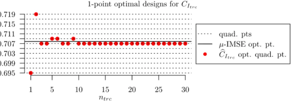
Figure 5.2.Representation of the 1-point optimal designs (quadrature-designs) forCbItrc as a
function ofntrc.
Table 5.1
Value, in percent, of the spectral ratioRbtrcfor variousntrc(Section5.1.1).
ntrc 1 2 3 7 9 10 15 36
b
Rtrc(%) 68.87 82.88 88.33 94.92 96.04 96.44 97.62 99.01
Figure 5.2shows the designsbt∗
ntrc optimal for CbItrc as a function of the number
ntrc of eigenvalues retained (for instance, for ntrc = 1, tb∗ntrc = 0.695); notice that
all these designs are quadrature-designs. A fast convergence ofbt∗ntrc to the µb
-IMSE-optimal designbt∗=bt∗Nq =0.707as ntrc increases is observed (a similar convergence
can also be observed for the 2-, 3- and 4-point design problems). For 3 6ntrc 69,
b
t∗ntrc oscillates between 0.707 and 0.709, the two quadrature points closest to the
µ-IMSE optimal designt∗. Forntrc>10,bt∗ntrc coincides withbt
∗=btq∗. Table5.1gives
the values, in percent, of the spectral ratio (quadrature approximation) for various truncation levelsntrc.
Remark 5.1 (Ornstein-Uhlenbeck process and quadrature approximation). For a one-dimensional centered Ornstein-Uhlenbeck process on Rand a quadrature µb, by considering the first and second derivative of the continuous function t 7→ CbI(Ht)
(these derivatives are defined whenever t is not a quadrature point), one can easily prove that one-pointµb-IMSE optimal designs are always quadrature-designs. /
5.1.2. Kernel of squared-exponential (Gaussian) type. We keep the same notation and setting as in Section5.1.1but we now assume that the centered Gaussian processZ admits the following covariance onR,
∀xandy∈R, K(x, y) =e−(x−y)
2
−e−(x2+y2).
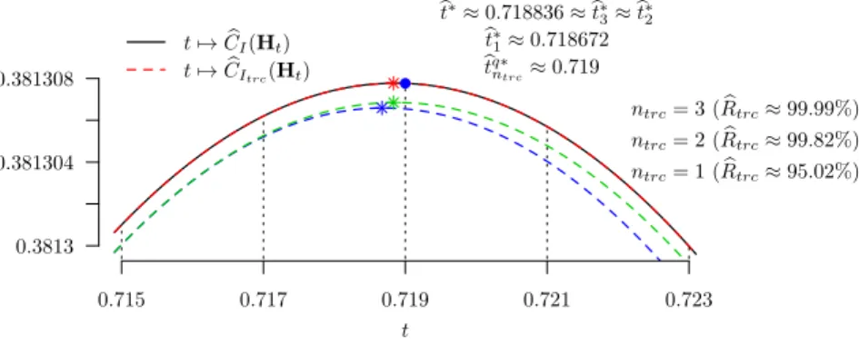
Figure5.3shows the values ofCbI(Ht)andCbItrc(Ht), withntrc∈ {1,2,3}, as functions
of the design pointt. The corresponding spectral ratios are reported on the figure. For any truncation level ntrc, the optimal 1-point quadrature-design is btqn∗trc =
b
tq∗ =0.719. Forn
trc = 1(bottom curve), the optimal design is bt∗1 ≈0.718672and
for ntrc > 2, we have bt∗ntrc ≈0.718836 ≈bt
∗. One may note that in this example,
the 1-point optimal designs forµb-IMSEtrcare not supported by the quadrature (i.e.,
are not quadrature-designs). However, we haveCbI(Hbt∗)≈0.3813078andCbI(Hbt∗)−
b
CI(Hbtq∗) ≈ 8.258e-09, so that the error induced by the restriction to
quadrature-designs is marginal.
0.3813 0.381304 0.381308 0.715 0.717 0.719 0.721 0.723 t7→CbI(Ht) t7→CbItrc(Ht) ntrc= 1 (Rbtrc≈95.02%) ntrc= 2 (Rbtrc≈99.82%) ntrc= 3 (Rbtrc≈99.99%) bt∗≈0.718836≈bt∗ 3≈bt∗2 b t∗ 1≈0.718672 b tq∗ ntrc≈0.719 t
Figure 5.3. Graphs of t7→CbI(Ht)and t7→CbItrc(Ht)(withntrc∈ {1,2,3}) around their
maximum, i.e., for0.7156t60.723.
Table 5.2
Value, in percent, of the spectral ratioRbtrcfor variousntrc(Section5.2).
ntrc 1 2 3 4 5 6 12
b
Rtrc(%) 74.81 85.72 96.63 98.23 98.96 99.70 99.99
5.2. Gaussian kernel on the unit square. Consider now a centered Gaussian processZ onR2 with covariance (Gaussian, or squared-exponential) kernel,
∀xandy∈R2, K(x, y) =e−kx−yk
2 ,
where k · k is the Euclidean norm ofR2. We take µ as the uniform probability on
[0,1]2 (so thatτ= 1).
We approximate integrals over[0,1]2through a quadrature consisting of a regular
grid of 33×33 points, all points receiving the same weight (mid-point rectangular quadrature rule). The corresponding discrete measure is denoted by µb. Table 5.2
gives the spectral ratiosRbtrc (in percent) for various truncation levelsntrc.
Figure 5.4 shows the quadrature-designs Xbq∗
n and Xbn,nq∗trc respectively optimal
for CbI and CbItrc, with ntrc = n (the design size) for n = 4 and n = 5; Xb q∗ n and
b
Xq∗
n,n coincide for n = 4 but not for n = 5. We numerically observe that the
5-point quadrature-designs optimal for CbItrc with ntrc > 6 are the µb-IMSE optimal
quadrature-design Xb5q∗. The right part of Figure 5.4 illustrates in particular how
b
CItrc(Xb q∗
5 ) tends to CbI(Xb5q∗) (dashed line on the top) when ntrc increases. Notice
that CbItrc(Xb q∗
5 )is an increasing function ofntrc and that forntrc= 6, CbItrc(Xb q∗ 5 )≈ 0.9890146, which is already very close ofCbI(Xb5q∗)≈0.9890174.
The 4- and 5-point bµ-IMSE optimal designs Xb4∗ and Xb5∗ (with quadrature
ap-proximation but without restriction to quadrature-designs) are not supported by the quadrature points. However, for the4-point problem, we obtain
b
CI(Xb4∗)≈0.9815098andCbI(Xb4∗)−CbI(Xb4q∗)≈ 2.258776e-05,
and for the5-point problem, we have
b
0.0 0.2 0.4 0.6 0.8 1.0 0.0 0.2 0.4 0.6 0.8 1.0 ntrc=n= 4 4-point optimal designs
quad. pts b
µ-IMSE opt. quad. des. c
CItrcopt. quad. des.
0.0 0.2 0.4 0.6 0.8 1.0 0.0 0.2 0.4 0.6 0.8 1.0 ntrc=n= 5 5-point optimal designs
DesignXcq∗ 5,5 DesignXcq∗ 5 6 8 10 12 14 0.982 0.984 0.986 0.988 ntrc c CItrc(Xc q∗ 5,5) c CItrc(Xc q∗ 5) c CI(Xc5q∗,5) = 0.9881732 c CI(Xc5q∗) = 0.9890174
Figure 5.4. Quadrature-designs optimal for the criteriaCbIandCbItrc forn=ntrc= 4(left)
andn=ntrc= 5(middle). Values of the criterionCbItrc for the two quadrature-designsXbq
∗
5 and
b
X5,5q∗ (respectively optimal forCbI andCbItrc withntrc= 5) as functions ofntrc(right).
In both cases, the error induced by the restriction of the design problem to quadrature-designs is therefore negligible.
5.3. Numerical experiments in dimension 6. Consider the 6-dimensional tensor-product Matérn covariance kernel K(x, y) = Q6i=1Kθi(xi, yi), where x = (x1, . . . , x6)and y = (y1, . . . , y6) are in R6 and where the kernels Kθi(·,·) are given
byKθi(xi, yi) = (1 + √
3|xi−yi|/θi) exp(− √
3|xi−yi|/θi), withθi>0.
We set(θ1, θ2, θ3, θ4, θ5, θ6) = (0.32,0.52,0.62,0.52,0.42,0.62)and take µ as the
uniform probability measure on[0,1]6. The use of regular grids to approximate
inte-grals on high dimensional spaces is prohibitive and we consider a quasi Monte-Carlo quadrature with Nq = 5 000 points obtained from a uniform Halton sequence (see,
e.g., [Nie92]), each point receiving the same weight 1/Nq. The computations have
been performed withR-64biton a 2012 Macbook Air equipped with a 1.8GHz Intel Core i5 processor and 4Gb RAM.
The low discrepancy grid is generated with theRfunctionrunif.halton(). Using the functioneigen(), the eigendecomposition ofQWtakes approximately4minutes (with a O(N3
q) complexity). The computation of the matrix Ω = QWQ requires
approximately 2 minutes. The IMSE and truncated-IMSE are encoded using (4.13) and Remark 4.1. The design covariance matrix K is inverted using the function
solve(). The IMSE criterion is thus encoded as follows (indicated for reproducibility
of the test):
IMSE<-function(Iq){ TAU-sum(solve(MatQ[Iq,Iq])*MatO[Iq,Iq]) }
where Iq is the index set Iq of a quadrature-design, MatQ and MatO stand for the
matricesQandΩ, andTAUis the trace termτ (here,τ = 1).
Table5.3indicates the median duration, over1 000repetitions, of one evaluation of the functionIMSE()at a random quadrature-design for various design sizes (we use the functionmicrobenchmark()). The median duration for the inversion of the matrix
Kis also indicated. As expected, we observe that once the preliminary computations are done (that is, for the IMSE, the computation of the matrices Q and Ω), the computational cost of one evaluation of the IMSE for any quadrature-design mainly corresponds to the inversion of the covariance matrix of the design.
Table 5.3
Median duration (over1 000repetitions, random quadrature-designs), in seconds, for one
eval-uation of the functionIMSE()for various design sizes (6-dimensional example) and median duration
for the inversion of the design covariance matrix.
design size 10-point 30-point 50-point 70-point 100-point
IMSE() 46.47e-6 131.27e-6 439.11e-6 1.128e-3 3.033e-3
K−1 37.31e-6 114.78e-6 369.21e-6 971.80e-6 2.694e-3
6. Concluding remarks. We have described how the IMSE criterion can be approximated by spectral truncation. When a (pointwise) quadrature is used to inte-grate the MSE and the design space is restricted to subsets of quadrature points, we have detailed a numerically efficient strategy for computing the IMSE and truncated-IMSE. Obviously, since preliminary calculations are required, the approach presents some numerical interest only if many criterion evaluations have to be performed, which is the case in particular for design optimization. A simulated-annealing algorithm for the computation of IMSE optimal designs that takes advantage of these considerations is presented in [GP14].
In its present form, the approach only applies to random fields with known mean. The extension to kernel-based interpolation models including an unknown parametric trend would enlarge the spectrum of potential applications and is under current inves-tigation. Also, note that the choice of a suitable quadrature takes a special importance here since quadrature-designs are subsets of quadrature points. The consideration of the errors induced by restricting the optimization to quadrature-designs and by ap-proximating the exact criteria CI and CItrc by their quadrature approximations CbI
andCbItrc should deserve further studies.
The interest of optimizing the truncated-IMSE (with appropriated truncation level) instead of the IMSE needs to be investigated more thoroughly. Indeed, numer-ical experiments (see [GP14]) indicate that for truncation levels slightly larger than the design size, the truncated criterion is easier to optimize than the original IMSE, and at the same time yields designs with high IMSE efficiency. The construction of optimal designs for the truncated-IMSE criterion should also be compared with the approach of [SP10] (optimal designs for a Bayesian linear model based on the main eigenfunctions of the spectral decomposition), and the connection between the two approaches deserves further investigations.
In the framework considered in Sections4and5, the IMSE, which corresponds to the integral of the kriging variance, is widely acknowledged as a most sensible criterion for choosing observation sites in Gaussian process models. However, it is seldom used for optimal design because it seems complicated (numerically costly) to evaluate. We hope that the present paper will contribute to popularize the use of this criterion to quantify the prediction uncertainty attached to a given design.
Acknowledgments. This work was supported by the the project ANR-2011-IS01-001-01 DESIRE (DESIgns for spatial Random fiElds), joint with the Statistics Departement of the Johannes Kepler Universität, Linz (Austria).
The authors want to thank the two anonymous reviewers for their valuable com-ments and suggestions that significantly improved the presentation.
Appendix A. Proofs of some lemmas and propositions.
Cauchy-Schwarz inequality inHand C-iii, we have, for allh∈ H, khk2L2= Z X (h|Kt)2Hdµ(t)6khk2H Z X K(t, t)dµ(t) =τkhk2H,
the integral ofh2being well-defined as the integral of a positive measurable function
(see for instance [Dud02]).
Proof of Lemma 3.2. The reproducing property of K(·,·) and the Cauchy-Schwarz inequality imply that, for allxandy∈ X,
K(x, y) = Kx KyH6 Kx H Ky H= p K(x, x)pK(y, y).
Combining this with conditions C-ii and C-iii, we obtain
Z X Z X K(x, y)2dµ(x)dµ(y)6 Z X K(x, x)dµ(x) 2 =τ2.
Let{ei, i∈I} be an orthonormal basis of L2(X, µ)(withI a general index set, not
necessarily countable), we have
Z X Z X K(x, y)2dµ(y)dµ(x) =Z X Kx 2 L2dµ(x) = Z X X i∈I Kx ei 2 L2dµ(x) = X i∈I Tµ[ei]2L26τ 2, (A.1)
the interchange between the sum and integral being justified by Tonelli’s theorem. So, the operatorTµ is a Hilbert-Schmidt operator onL2(X, µ)andTµ is thus a compact
operator onL2(X, µ)(in particular, the number of terms different from 0 in the sum
on the right-hand side of (A.1) is at most countable). Finally, from the properties of symmetry and positivity ofK(·,·), we have, forf andg∈L2(
X, µ), fTµ[g]L2 = Tµ[f] gL2 and f Tµ[f]L2>0,
so thatTµ is self-adjoint and positive onL2(X, µ).
Proof of Proposition3.1. First, H0 is well-defined thanks to Lemma 3.1. Also note
that, as an orthogonal subspace, Hµ is by definition closed in H. For a fixed f ∈
L2(X, µ), we consider the linear functionalI
f,µ onHdefined by, ∀h∈ H, If,µ(h) =
Z
X
f(t)h(t)dµ(t).
Again,If,µis well-defined thanks to Lemma3.1. From the Cauchy-Schwarz inequality
and (3.2), we have
|If,µ(h)|6kfkL2khkL26
√
τkfkL2khkH,
so that the applicationIf,µ is continuous onH. Thus, from the Riesz-Fréchet
Theo-rem, there exists a unique elementρf,µ ofHsuch thatIf,µ(h) = (h|ρf,µ)H. One can
finally identifyρf,µ withTµ[f]thanks to
If,µ(h) = (h|f)L2= (h|Tµ[f])H, (A.2) 17
see [GB12] for more details. Equation (A.2) proves in particular that, for all f ∈ L2(
X, µ), Tµ[f]∈ H⊥H
0 =Hµ, since we have (using the Cauchy-Schwarz inequality) ∀f ∈L2(X, µ),∀h0∈ H0, h0|Tµ[f]H=(h0|f)L2
6kh0kL2kfkL2 = 0.
Denote bynull (If,µ)the null space ofIf,µ(which is closed inHas the null space
of a continuous linear application). We then remark that
H0=
\
f∈L2(X,µ)
null (If,µ),
so thatH0 is closed inH(and in particular, H⊥µH=H0).
Now, letkandl∈I+ and denote byδkl the Kronecker delta, we have (φk|φl)H= 1 λkλl Z X Z X e φk(x)φel(t)K(x, t)dµ(x)dµ(t) = λk λkλl δkl,
so that√λkφk, k∈I+ is an orthonormal system inHµ.
To conclude, suppose thath∈ H is such that(h|φk)H = 0 for all k∈ I+, then
Tµ[h] = 0. Since, from equation (A.2),khk2
L2 = (h|Tµ[h])H, we obtain that h∈ H0
and finally thatspan{φk, k∈I+}is dense inHµ. Proof of Lemma 4.1. The expression H
b
µ = spanKsj,16j6Nq follows directly
from the definition of bµ given in (4.7) (in particular because the support of µb is a finite set). By construction, we haveφbk∈ Hbµ for all16k6Nq and
∀x∈ X, Tbµbφk(x) =qT(x)WQQ−1vk =qT(x)Q−1QWvk =λbkφbk(x).
Finally, since(q|qT)
H=Q(matrix notation), we have
bφk 2 H=v T kQ−1QQ−1vk =vTkWW−1Q−1vk = 1 b λk vTkWvk= 1 b λk
and the orthogonality of theφbk can be obtained with similar arguments. Appendix B. Some technical remarks.
Remark B.1. The results of this paper can be extended to a non separable Gaussian Hilbert space H. However, in this case condition C-i is not sufficient to ensure the measurability of the functionx7→E(PHD[Zx])
2for a non-separable subspaceH D.
We then have to assume thatx7→K(x, x)is measurable (see for instance [For85]) and also, either restrict the definition of the IMSE to separable closed linear subspaces of
Hor assume that x7→E(PHD[Zx])
2is measurable whateverH D.
Note that the separability assumption forHis not very restrictive for most prac-tical situations. Indeed, from the structure theorem for Gaussian measures and the theory of abstract Wiener spaces, this assumption is satisfied by all random fields with sample paths in classical functions spaces, such as Banach or Fréchet spaces, see
for instance [Sat69,DFLC71,Bor76]. /
Remark B.2. To ensure thatCI(HD)is well-defined, we have to check the
measura-bility of the functionx∈ X 7→E(PHD[Zx])
2. From the isometry betweenH Dand HD, if{hj, j∈J} is an orthonormal basis ofHD, then we have, for all x∈ X,
06E(PHD[Zx])
2=X
j∈J
h2
The functionx7→Pj∈Jh2
j(x)is well-defined and is measurable as an at most
count-able sum of (positive) measurcount-able functions (sinceH is separable). Finally CI(HD)
is well-defined as the integral of a positive mesurable function. Note that a similar reasoning with HD = H shows that RXK(x, x)dµ(x) is well-defined assuming C-i
(andHseparable). /
REFERENCES
[ABM12] Y. Auffray, P. Barbillon, and J.-M. Marin. Maximin design on non hypercube domains and kernel interpolation. Statistics and Computing, 22:703–712, 2012.
[Bor76] C. Borell. Gaussian Radon measures on locally convex spaces. Mathematica Scandi-navica, 38:265–284, 1976.
[BT04] A. Berlinet and C. Thomas-Agnan. Reproducing Kernel Hilbert Spaces in Probability
and Statistics. Kluwer, Boston, 2004.
[CS02] F. Cucker and S. Smale. On the mathematical foundations of learning.Bulletin (new
series) of the American Mathematical Society, 39(1):1–49, 2002.
[DFLC71] R.M. Dudley, J. Feldman, and L. Le Cam. On seminorms and probabilities, and abstract Wiener spaces. Annals of Mathematics, pages 390–408, 1971.
[DPZ13] H. Dette, A. Pepelyshev, and A. Zhigljavsky. Optimal design for linear models with correlated observations. The Annals of Statistics, 41(1):143–176, 2013.
[Dud02] R.M. Dudley.Real Analysis and Probability, volume 74. Cambridge University Press, 2002.
[For85] R.M. Fortet. Les opérateurs intégraux dont le noyau est une covariance.Trabajos de
Estadistica y de Investigacion Operativa, 36:133–144, 1985.
[GB12] B. Gauthier and X. Bay. Spectral approach for kernel-based interpolation. Annales
de la faculté des sciences de Toulouse, 21 (num. 3):439–479, 2012.
[GP14] B. Gauthier and L. Pronzato. Approximation of IMSE optimal designs of experiments via quadrature rule and spectral decomposition.
Communi-cations in Statistics – Simulation and Computation, 2014. To appear,
http://hal.archives-ouvertes.fr/hal-00936681.
[Hac95] W. Hackbusch. Integral Equations: Theory and Numerical Treatment, volume 120. Birkhäuser, Basel, 1995.
[Kre99] R. Kress. Linear Integral Equations, volume 82. Springer, New York, 1999.
[LMK10] O.P. Le Maître and O.M. Knio. Spectral Methods for Uncertainty Quantification. Springer, 2010.
[Nie92] H. Niederreiter. Random Number and Quasi-Monte Carlo Methods. SIAM, Philadel-phia, 1992.
[R C13] R Core Team. R: A Language and Environment for Statistical Computing. R Foun-dation for Statistical Computing, Vienna, Austria, 2013.
[RW06] C.E. Rasmussen and C.K.I. Williams. Gaussian Processes for Machine Learning. MIT press, Cambridge, MA, 2006.
[S+13] W.A. Stein et al. Sage Mathematics Software (Version 5.6). The Sage Development
Team, 2013. http://www.sagemath.org.
[Sat69] H. Satô. Gaussian measure on a Banach space and abstract Wiener measure.Nagoya
Mathematical Journal, 36:65–81, 1969.
[Sch79] L. Schwartz. Analyse Hilbertienne. Hermann, 1979.
[SP10] G. Spöck and J. Pilz. Spatial sampling design and covariance-robust minimax predic-tion based on convex design ideas. Stochastic Environmental Research and Risk
Assessment, 24(3):463–482, 2010.
[ST06] C. Schwab and R.A. Todor. Karhunen-Loève approximation of random fields by gen-eralized fast multipole methods. Journal of Computational Physics, 217(1):100– 122, 2006.
[SWMW89] J. Sacks, W.J. Welch, T.J. Mitchell, and H.P. Wynn. Design and analysis of computer experiments. Statistical Science, 4(4):409–423, 1989.
[SY66] J. Sacks and D. Ylvisaker. Designs for regression problems with correlated errors.
The Annals of Mathematical Statistics, pages 66–89, 1966.
[Wah90] G. Wahba. Spline Models for Observational Data, volume 59. SIAM, Philadelphia, 1990.