MPRA
Munich Personal RePEc Archive
The Dynamics of Spending and
Absorption of Aid: Panel Data Analysis
Abu Shonchoy
IDE-JETRO
5. August 2010
Online at
https://mpra.ub.uni-muenchen.de/24530/
INSTITUTE OF DEVELOPING ECONOMIES
IDE Discussion Papers are preliminary materials circulated
to stimulate discussions and critical comments
Keywords:Aid, Spending and Absorption, PRGF, Dynamic Panel Estimations. JEL classification:F34, F35
*
Research Fellow, Poverty Alleviation and Social Development Studies Group, Inter-disciplinaryIDE DISCUSSION PAPER No. 245
The Dynamics of Spending and
Absorption of Aid: Panel Data Analysis
Abu S SHONCHOY*
August 2010
Abstract
In September 1999, the International Monetary Fund (IMF) established the Poverty Reduction and Growth Facility (PRGF) to make the reduction of poverty and the enhancement of economic growth the fundamental objectives of lending operations in its poorest member countries. This paper studies the spending and absorption of aid in PRGF-supported programs, verifies whether the use of aid is programmed to be smoothed over time, and analyzes how considerations about macroeconomic stability influence the programmed use of aid. The paper shows that PRGF-supported programs permit countries to utilize all increases in aid within a few years, showing smoothed use of aid inflows over time. Our results reveal that spending is higher than absorption in both the long-run and short-run use of aid, which is a robust finding of the study. Furthermore, the paper demonstrates that the long-run spending exceeds the injected increase of aid inflows in the economy. In addition, the paper finds that the presence of a PRGF-supported program does not influence the actual absorption or spending of aid.
The Institute of Developing Economies (IDE) is a semigovernmental,
nonpartisan, nonprofit research institute, founded in 1958. The Institute
merged with the Japan External Trade Organization (JETRO) on July 1, 1998.
The Institute conducts basic and comprehensive studies on economic and
related affairs in all developing countries and regions, including Asia, the
Middle East, Africa, Latin America, Oceania, and Eastern Europe.
The views expressed in this publication are those of the author(s). Publication does not imply endorsement by the Institute of Developing Economies of any of the views expressed within.
INSTITUTE OF DEVELOPING ECONOMIES (IDE), JETRO 3-2-2, WAKABA,MIHAMA-KU,CHIBA-SHI
CHIBA 261-8545, JAPAN
©2010 by Institute of Developing Economies, JETRO
The Dynamics of Spending and Absorption of Aid:
Panel Data Analysis
∗Abu S. Shonchoy†
Institute of Developing Economies, JETRO, Chiba, Japan and University of New South Wales, Sydney, Australia
August 5, 2010
Abstract
In September 1999, the International Monetary Fund (IMF) estab-lished the Poverty Reduction and Growth Facility (PRGF) to make the reduction of poverty and the enhancement of economic growth the fundamental objectives of lending operations in its poorest mem-ber countries. This paper studies the spending and absorption of aid in PRGF-supported programs, verifies whether the use of aid is pro-grammed to be smoothed over time, and analyzes how considerations about macroeconomic stability influence the programmed use of aid. The paper shows that PRGF-supported programs permit countries to utilize all increases in aid within a few years, showing smoothed use of aid inflows over time. Our results reveal that spending is higher than absorption in both the long-run and short-run use of aid, which is a robust finding of the study. Furthermore, the paper demonstrates that the long-run spending exceeds the injected increase of aid inflows in the economy. In addition, the paper finds that the presence of a PRGF-supported program does not influence the actual absorption or spending of aid.
Keywords: Aid, Spending and Absorption, PRGF, Dynamic Panel Estimations.
JEL Classification: F34, F35.
∗
Acknowledgement: I am particularly thankful to Markus Berndt, Jan Kees Martijn, Andy Berg with whom I had many and very useful discussions on this topic. I would also like to thank Stefania Fabrizio, Patricia Alonso-Gamo, and other participants of internal seminars at the IMF. My heartfelt thanks goes to them. Usual disclaimers apply.
†
1
Introduction
Aid is a useful tool that facilitates the transfer of resources from one country to another. It enables recipient countries - predominantly developing coun-tries - to increase consumption and investment. Aid provides an opportunity to reduce poverty, increase the standard of living and generate sustainable economic growth. However, concern for the effective utilization and manage-ment of aid dollars in recipient countries has recently been expressed. The imperative to employ aid inflows adequately may stress the administrative capacity of governments. In addition, volatile aid flows create problems of financial management and debt sustainability in the future.
Unlike the international flow of capital, aid money is initially held by the central bank. Governments then can decide whether or not to increase pub-lic spending by running a greater fiscal deficit. At the same time, central banks can choose whether or not toabsorb aid inflows by selling aid dollars and widening current account deficits. Although most of the aid literature assumes that absorption and spending of aid is equivalent, spending could be different from absorption due to the lack of stark agreement and coor-dination between the government and the central bank. Such asymmetry between spending and absorption could have quite adverse macroeconomic consequences (Berg et al. 2005).
Questions could therefore arise regarding the advice offered by the IMF to their member countries about the use of aid inflows. Further issues could arise on how considerations of aid volatility, capacity constraints and macroeconomic stability could shape these recommendations. To address these questions, we took as a case the Poverty Reduction and Growth Facil-ity (PRGF) program, an IMF-supported aid program that plays a catalytic role in unlocking aid dollars to achieve poverty reduction and growth en-hancement. The objective of this study is to estimate the programmed spending and absorption of aid for PRFG arrangements. Placing the em-phasis on programmed spending rather than actual spending, this study estimates how much spending and absorption is determined by the program design in countries that have a PRGF in place. Furthermore, this study studies whether or not actual spending and absorption is affected by the PRGF program.
A pioneering study on estimating programmed spending and absorption of a PRFG-supported program has been undertaken by Dudine et al. (2008). The estimation used in their paper predominantly used pooled estimation techniques which created biased estimations due to the presence of lagged dependent term as one of the regressors in the model. Nevertheless, by using the same dataset, the present study has improved on the estimations of Dudine et al. (2008) and is able to provide efficient estimates and additional insights to this area of study.
This study uses the IMF spending and absorption dataset in estimating re-duced form models. The dataset contains data from staff reports concerning requests for, or reviews of, all PRGF programs that were approved during the period 1999-2007. The dataset is an unbalanced panel data from 369 program documents of 51 developing countries which allows tracking of the IMF’s projections and economic programming. If the IMF employs any rule that suggests to countries how aid dollars should be spent and absorbed, this dataset would allow such a rule to be deduced. Some variables in the dataset have been collected from the World Economic Outlook (WEO) to control for other variables that are not generally reported in the program documents.
The study demonstrates that PRGF-supported programs permit countries to utilize all increases in aid within a few years, showing smoothed use of aid inflows over time. Our results reveal that spending is higher than absorption in both the long-run and short-run use of aid, which is a robust finding of the study. Furthermore, the study finds that the long-run spending exceeds more that the injected increase of aid into the economy. In contrast, we find weak evidence of profound influence of other control variables on the spending and absorption of aid. Finally, the study finds that the presence of a PRGF-supported program does not influence the actual absorption or spending of aid.
The study is organized as follows. Section 2 elucidates the concept of ab-sorption and spending, and the macroeconomic consequences of aid inflows to developing countries. Section 3 describes the PRGF program of IMF to its member countries. Section 4 introduces the key elements of the method-ological framework of the estimations. Section 5 gives a brief description of
the dataset and control variables used in this study. Section 6 presents the estimation results and section 7 concludes.
2
Conceptual Framework
The macroeconomic impact of aid inflows typically depends on the pol-icy choices of government authorities. Specifically, the interaction of fiscal, monetary and exchange rate policy shapes the use and impact of aid in the recipient countries. To facilitate the understanding of this interaction, two useful concepts of ‘Absorption’ and ‘Spending’ have been introduced by Berg et al. (2007) where the current account response is measured by a ratio of aid absorption and the fiscal response is measured by a ratio of aid spend-ing (Dudine et al. 2008). Applying Berg et al. (2007), Aiyar and Ruthbah (2008) and Hansen and Headey (2009), we used an accounting framework utilizing the balance of payments and the national accounting system, in-stead of originating a theoretical model to identify the mediums by which aid inflows have an effect on macroeconomic aggregates.
2.1 Absorption
Using the balance of payments system, aid inflows in the form of grants are booked as a current transfer on the record of current accounts whilst loans are booked on the capital account. Hence, using the simple balance of payments identity we can express the following equations
CABt+KABt= ∆Rt. (1)
Where
CABt= (Xt−Mt) +Wt−(itLt−1+rtDt−1) +Agt, (2)
and
KABt= ∆L0t + (Alt−Art). (3)
In equation 1, CAB is the current account balance, KAB is the capital account balance andR is the foreign reserves. The current account balance is specified in equation 2, as the net export (export X, minus import M)
plus net private transfersW (mostly remittances and worker compensations) less net interest payments to foreigners (iL+rD), where separate interest payments on market loans (iL) and aid loans (rD) have been used. The last term in equation 2 is the aid grants (Ag). The capital account balance comprises net change in non-aid foreign debt (∆L0,having both private and public component) in addition to the aid loan given in a year (Al) minus the repayment of principal on the aid loans (Ar) which is known as amortization. Here subscript tdenotes year.
Separating the factors of aid from equation 2 and 3 and rearranging these three equations yields:
Agt +Alt−Art | {z } AID Inflows = ∆Rt−[(Xt−Mt) +Wt−(itLt−1+rtDt−1)] | {z } NACAB − ∆L0t | {z } NAKAB (4)
where NACAB is the non-aid current account balance and NAKAB is the non-aid capital account balance. The aid inflows are the sum of grants and loans less the repayment.1 Thus an increment in net aid inflow, either grant
or loan, can affect the economy in the following ways. It can:
1. Enhance the international reserves;
2. Increase the non-aid current account deficit through net imports of good and services;
3. Finance the payments of interest on foreign debt (both aid and non-aid debt);
4. Finance a reduction in private transfers; and
5. Raise non-aid capital outflows (capital flight).
Realistically, aid will not have any counterpart in increased consumption or investment if the aid dollars are entirely utilized for augmenting foreign reserves or financing capital outflows. Hence, under conventional condi-tions, the most usual application of aid inflows, as a measure of the direct resource transfer, is to finance a widening of the current account deficit. Thus, absorption is the decline in the non-aid current account balance that
1This concurs with the Development Assistance Committee (DAC) definition of net
Official Development Aid (ODA): net ODA =Agt +A
l t−Art.
is determinable to aid. More formally,
Absorption= ∆NACAB
∆Aid . (5)
Berg et al. (2007) discussed how absorption predominately depends on cen-tral bank decisions on reserve aggregation and on the interest rate, which further acts upon the demand for private sector imports. Some exceptions to central bank dominance of aid inflows are aid-in-kind, aid given directly to the government for buying imported goods and services and aid directly given to NGOs, in which case the aid is fully absorbed. Interestingly, there is no event of absorption for the grant of debt forgiveness. However, such exceptions are quite irregular, leaving the majority of the decisions on ab-sorbtion of the aid inflows to the central bank.
2.2 Spending
Utilizing national account identities, spending catches the magnitude by which the aid inflow is utilized to finance an increase in government expen-diture or a decrease in taxation. Using fiscal side definitions,
Fiscal Balance =Gt−Tt−At−Domestic Finance, (6)
which makes
Fiscal Deficit=Gt−(Tt−At), (7)
where G is the government expenditure, T is the domestic revenue and A
is the aid inflows. Now deducting aid inflows (A) from the both side of the equation 7 yields,
Non-Aid Fiscal Deficit (NAFD)=Gt−Tt. (8)
Hence, with an increment of net aid inflows, governments can either
1. Reduce domestic revenues,
2. Increase government expenditure, or
Thus, spending is the decline in the non-aid fiscal deficit that is determinable to aid. More formally,
Spending = ∆NAFD ∆Aid .
Although aid sometimes comes as non-fungible project assistance, govern-ments can take the decision whether or not to enhance the overall fiscal deficit as aid increases, which is largely the settlement of the fiscal authori-ties.
2.3 Spending and Absorption
Since spending and absorption are dealt with by different authorities, spend-ing will be different from absorption, if perfect agreement and co-ordination are absent, although there are some cases such as aid in kind and aid ded-icated to finance government import, in which spending will be equal to absorption. Such cases do not have any effect on macroeconomic variables such as the exchange rate, interest rate and price level (Aiyar et al. 2005), but other than such obvious examples, the policy response to the aid inflows results in different combinations of spending and absorption, providing var-ious macroeconomic consequences. In line with Dudine et al. (2008), a brief summary of such consequences of spending and absorption is expressed be-low.2
The spending and absorption of aid are the same when the widening of the current account deficit acts in line with the fiscal deficit. In this case, the increased fiscal net demand is fulfilled by increasing net imports. However, there are cases where absorption will be higher than spending if central bank authorities decide to sell more foreign exchanges associated with increased aid inflows than is necessary. Such increases in the sell of foreign exchanges are utilized to finance domestic debt which has occurred as a result of higher government spending. This leads to sluggish monetary growth, appreciated real exchange rate, lower inflation and reduced interest rate. The end re-sult will be increased private consumption and higher domestic investment,
2
Berg et al. (2007) and Aiyar and Ruthbah (2008) discuss the macroeconomic conse-quences of various combinations of spending and absorption in detail.
which may increase net imports.
In contrast, spending could be greater than absorption when central bank authorities decide to sell fewer foreign exchanges associated with increased aid inflows than is necessary. In this case, fiscal deficit increases due to higher government spending, but aid is accumulated to build the central bank’s foreign reserves. Fiscal authorities are financing the widening of fiscal deficit through domestic borrowing, which results in a depreciated real exchange rate, higher inflation and a greater interest rate. This leads to lower consumption and private investment, and tends to shift resources from the private sector to the public sector; thus, spending will be greater than absorption.
The total net foreign aid disbursed by donor countries has increased over the years, but this has been followed by growing aid volatility in both the an-nouncement and disbursement of aid (Aslam and Kim 2007). ? have demon-strated that macroeconomic management of poor, aid-dependent countries becomes extremely difficult with the high level of volatility in aid inflows. They find that aid disbursements have typically been pro-cyclical, indicating the failure of aid as a stabilizer or as an insurance against large macroeco-nomic shocks (for example in case of natural disasters). As a result, it might be optimal for the recipient countries not to utilize all the increments in aid inflows at once, but to smooth them over time. Similarly, when capacity constraints are stark or the level of inflation is high, large government ex-penditures due to aid surge might use up the productive capability of the economy and exacerbate pressure on inflation. A temporary policy of ab-sorbtion but not spending could therefore help countries to reduce inflation or the high level of domestic debt to a position where aid can be used without harming macroeconomic stability. Likewise, in the case of low international reserves, a temporary strategy could be to employ part of the aid increments to build up a reserve buffer that would facilitate spending for countries that are facing aid volatility.3
Recent literature on absorption and spending of aid inflows uses both nar-rative and empirical approaches to understand the macroeconomics of aid. Leading this literature is the seminal work by Berg et al. (2005) in which
3
they used a small number of elaborated case studies of countries that have recently experienced prominent scaling-up in actual aid inflows. The study finds that, spending is typically greater than absorption for the aid recipi-ent countries, resulting in the domestic expenditure being higher than the net imports. Extending this approach, Foster and Killick (2006) also drew the same conclusion. Improving on Berg et al. (2005), Aiyar and Ruth-bah (2008) systematically analyzed the spending and absorption of actual aid, using the econometric analysis of a cross-section of countries. They employed dynamic a panel data framework to estimate both short-run and long-run absorption and spending. The work of Aiyar and Ruthbah (2008), in principle, supports the conclusion of Berg et al. (2007) and Foster and Killick (2006), which contradicts the conventional view of full spending and absorption.
A subsequent study on the programmed use of aid increases was included in the IEO (2007) report. This study finds that programmed spending and ab-sorption in Sub-Saharan Africa (SSA) countries under the PRGF-supported program is rather limited. However, the paper only used same-year use of aid increases, which made the paper’s conclusion questionable. Further to the IEO (2007) study, Dudine et al. (2008) used a new and comprehen-sive database for all countries with PRGF arrangements to estimate the programmed use of aid. They concluded that PRGF allows countries to smooth the use of almost all increments of aid inflows over time. Contra-dicting the finding, a recent study by Hansen and Headey (2009) argues that absorption is somewhat equal to spending in the case of small developing countries. They also observed that aid is neither spent nor absorbed in any systematic manner by the non-aid dependent countries. Hence the literature draws mixed conclusions on the actual and programmed use of aid inflows by recipient countries, and improved methodology and a comprehensive dataset is required to draw a cohesive conclusion on this issue.
3
PRGF Aid Program
In September 1999, the International Monetary Fund (IMF) established the Poverty Reduction and Growth Facility (PRGF), replacing the Enhanced Structural Adjustment Facility (ESAF). The aim of the PRGF is to make
the reduction of poverty and the enhancement of economic growth the fun-damental objectives of the lending operations of the IMF in its poorest member countries. The principal features of the PRFG program, as stated in PDR (2000) are:
1. Broad participation and greater ownership,
2. Embedding the PRGF in the overall strategy for growth and poverty reduction,
3. Budgets that are more pro-poor and pro-growth,
4. Ensuring appropriate flexibility in fiscal targets,
5. More selective structural conditionality,
6. Emphasis on measures to improve public resource management/accountability, and
7. Social impact analysis of major macroeconomic adjustments and struc-tural reforms.
Each year during the period 1999-2007, a PRGF program was in place for 25 to 40 countries; typically a three year program which usually set macroe-conomic targets for the medium term. Under this arrangement, successive economic reports were presented to the Board of the IMF: the first when a country requested a PRGF program and subsequently when performance under the program was evaluated. This program evaluation, known as ‘Pro-gram Review’ was typically carried out by IMF country offices every six months. Program reviews included both fiscal and balance of payments projections and a set of program conditions. Such quantitative national in-come and balance of payments projections were coherent with the intended policies of the government authorities and supported by the IMF. The pro-gram conditions were placed to ensure two objectives: tracking the progress in enforcing the intended policies of the government authorities and ensur-ing the set conditions were met to unlock the schedule disbursements by the IMF. These conditions and policies continue to be in force today for PRFG programs.
Program projections and conditions implicitly determine the use of the an-ticipated aid inflows and are termed ‘programmed use of aid’ in this study. This program generally sets a base on the build-up of international reserves and a cap on some measure of the fiscal deficit or fiscal financing, thus de-termining the capacity by which projected aid can be utilized to finance higher net imports and fiscal spending. However for many reasons, the ac-tual use of aid may be substantially different than was planned under the PRGF. Even when program conditions are met, the actual fiscal and cur-rent account deficit could be greater (or smaller) than the projection. Such deviation could arise, for example, if capital inflows are different from what was expected, or if unanticipated aid shocks (positive or negative) occur. A mechanism is included in the program design to automatically adjust the program conditions in adapting the unexpected aid inflows. Hence, most programs permit greater spending in aid windfalls and do not require lower spending in aid shortfalls.
In measuring the aid inflows, this study takes a practical approach by includ-ing all official net transfers and loans under the concept of aid, since from a macroeconomic perspective, aid is the transfer of resources from donors to recipient countries. Aid may take several forms, such as both grants and loans, budget support and non-fungible project financing, which may not be channeled through the government budget in the recipient country. To calculate aid inflows, net official borrowing is added with official transfers and grants, and the interest payments to official creditors are deducted from the sum. Furthermore, the flow component of alleged ‘exceptional financing’ is also added to the accounting of the aid inflows.4 Hence, this study com-putes aid inflow on a cash basis to appropriate the net transfer of financial resources from donors to recipient countries.
4
Methodology
Following the IEO (2007) and Aiyar and Ruthbah (2008) approach, the following models have been used to capture the absorption and spending of
4
Exceptional financing is the part of debt relief that is not used for clearing arrears. Such financing is available to pay for imports or debt services.
aid:
∆NACABi,t =α1+β1∆AIDi,t+ K
X
k=1
δ1kXk+γYeart+µ1i+i,t (9)
∆NAFDi,t =α2+β2∆AIDi,t+ K
X
k=1
δ2kXk+γYeart+µ2i+i,t. (10)
Whereidenotes the country, tdenotes time (which is uniquely ranked and based on the date the document was published) and ∆ denotes the differ-ence between the programmed level and actual level. For example, the term ∆NACABi,tcan be elaborated as NACABi,t(programmed)−NACABi,t−1(actual).
Continent-specific dummies are used to capture the unobserved time inde-pendent constant effect (µi) as Putman (1993) and Acemoglu et al. (2001)
argued that current political, social and economic institutions of many coun-tries have largely been determined by their past history, geography and reli-gion. Also, all the regression estimations have year-specific dummies which have accommodated the year-specific variation in the model. Xk is a vector
of control variables of sizeK.
Similarly, we used the following alternative models in levels to estimate the fraction of the aid inflows that is programmed to be absorbed and spent over time:
NACABi,t =α3+β3AIDi,t+ K
X
k=1
δ3kXk+γYeart+µ3i+i,t (11)
NAFDi,t =α4+β4AIDi,t+ K
X
k=1
δ4kXk+γYeart+µ4i+i,t. (12)
Here, the parameters of interest are βs since they capture the short run absorption and spending of aid inflows. One may argue that the dependent variables of the aforementioned equations also depend on their past values. In that case, we need to use the lag dependent variable as a regressor to capture the level of persistency in the regression. Such inclusions convert the above equations into Dynamic Panel Data (DPD) models. In the case
of absorption and spending, the equations become,
∆NACABi,t =α5+β5∆AIDi,t+ρ5∆NACABi,t−1+
K
X
k=1
δ5kXk+γYeart+µ5i+i,t
(13)
∆NAFDi,t =α6+β6AIDi,t+ρ6∆NAFDi,t−1+
K
X
k=1
δ6kXk+γYeart+µ6i+i,t.
(14)
Likewise, by introducing the lagged dependent variable as regressor, the alternative models in levels become
NACABi,t=α7+β7AIDi,t+ρ5NACABi,t−1+
K
X
k=1
δ7kXk+γYeart+µ7i+i,t,
(15)
NAFDi,t=α8+β8AIDi,t+ρ8NAFDi,t−1+
K
X
k=1
δ8kXk+γYeart+µ8i+i,t.
(16)
Here ρs capture the level of persistence of the lagged dependent variable. To test the hypothesis of cross-sectional independence in panel-data mod-els with small T and large N, we employed semi-parametric tests proposed by Friedman (1937) and Frees (1995, 2004) as well as the parametric test-ing procedure proposed by Pesaran (2004).5 Results of these tests showed
evidence of contemporaneous correlation across the units. We also found evidence of group-wise heteroscedasticity and serial correlation in the er-ror terms (using a modified Wald test and Wooldridge test). To estimate equations 9 to 12, we used the Feasible Generalized Least Square (FGLS) method with correction for panel specific AR1 process (within panels) and heteroscedasticity (across panels).
Equations 13 to 16, on the other hand, cannot be consistently estimated using FGLS or OLS due to the presence of lagged dependent term as one of the regressors. Due to the endogenous nature, the lagged dependent variable is correlated with the error term of the estimation which creates a large-sample bias in the estimation (Nickell 1981). Estimation bias could also arise if the lagged dependent variable is correlated with the regressors, even if the
5We used xtcsd routine in STATA, developed by De Hoyos and Sarafidis (2006) to
error process is i.i.d. However, if the error process is autocorrelated then the problem becomes even more serious (Baum 2006). To address such problems, an application of General Methods of Moments (GMM) estimator, proposed by Blundell and Bond (1998), is utilized where they suggested to use a system of equations using lagged levels as well as lagged differences for the DPD estimations.6 These equations differ in their moment conditions and the set of instruments used. Here, predetermined and endogenous variables (in first difference) are instrumented with lags of their own levels. Similarly, lags of own first difference are used to instrument the predetermined and endogenous variables (in levels). A detail description and application of the Blundell and Bond (1998) estimator can be found in Roodman (2006).
5
Data and Variables
5.1 Data description
The dataset is available from the IMF website and contains data from staff reports of all PRGF programs that have been approved over the 1999-2007 period.7 In the dataset, each observational unit is the country and un-der each unit there are document-specific data for different variables. The dataset is an unbalanced panel based on the data from 369 program doc-uments of 51 developing countries. As explained in Section 3, a program document has the record of projections and actual data that were formally agreed upon with the authorities and presented to the Board of the IMF. Ranging from 1996 to 2010, the dataset contains actual data from the oldest document (1999) to three years’ projections for the most recent documents (2007). Some variables in the dataset are collected from the World Eco-nomic Outlook (WEO) to control for other variables that are not generally reported in the program documents (for example, data on terms of trade and PPP-adjusted real per capita GDP).
In the dataset, aid is constructed using both a national accounting and balance of payments approach. The variable ‘fiscal-aid’ is constructed as
6
Blundell and Bond’s system estimator, also known as ‘System GMM’, is an extension of the Arellano and Bond (1991) estimator.
7
the net foreign financing including grant, debt relief and the flow compo-nent of exceptional financing. The ‘bop-aid’ is derived by adding changes in liabilities to official creditors (disbursements − amortization) to official current transfers and capital transfers with the programmed financing gap, increases in external arrears, rescheduling and other balance of payments or fiscal supports. External interest payments are then deducted from this amount.
The fiscal deficit net of aid is constructed from the difference between ex-penditures excluding interest payments and revenue excluding grants. The current account deficit net to aid is derived by excluding official current transfers and interest payments from the current account balance. Both aid and the fiscal and current account deficits are expressed as a share of GDP. The details of the data collection process, the countries and documents used to construct the dataset are well documented in Dudine et al. (2008).
5.2 Control Variables
For the spending regressions, we controlled for the lagged changed in fiscal deficit (net to aid), lag of overall fiscal deficit, real GDP growth and the lag of the inflation rate. The first control variable is used to capture the indirect effect of past aid on the current fiscal deficit (net of aid). Inclusion of this variable also captures the concern of the fiscal authorities in keeping the level of deficit stable. The lag of overall fiscal deficit captures the concerns about fiscal consolidation. A negative coefficient implies that the greater the overall fiscal deficit in the past, the lower the programmed fiscal deficit net of aid. Real GDP growth controls for the cyclicality of fiscal policy. A negative coefficient entails higher deficit is programmed when economic growth slows down. Finally, the lag of inflation rate captures the impact of fiscal policy on internal macroeconomic stability; thus, a negative coefficient implies that as past inflation is higher, the larger is the programmed reduction in the fiscal deficit.
Similarly, for absorption equations, we controlled for lagged change in the current account deficit (net of aid), lag of overall current account deficit, the lag change in the term of trade, the change of overall fiscal deficit, per capita GDP (relative to that of the US) and the lag of reserve coverage in term
of months of import. The first control variable is utilized to capture the indirect effect of past aid on the current account deficit. The lag of overall current account deficit is employed for the same reason as described for the overall fiscal deficit in the spending regressions. The lag change in the terms of trade captures the concern about adjusting to past exogenous shocks. A positive coefficient implies that past shocks are permitted to contribute to the economy through an increase in current account deficit net of aid. The change in the overall fiscal deficit is used to control for the demand pressures created by the fiscal policy on the current account. Per capita GDP controls the vulnerability; the higher the per capita income of a country, the more resilient the country is to shocks. A positive coefficient implies that a larger increase in the current account deficit is programmed for countries with high per-capita income. Finally, the lag of reserve coverage is used to capture the external stability, particularly reserve adequacy. A positive coefficient means that a greater increase in the current account deficit is programmed for those countries where the reserve accumulation is sufficiently large. All these control variables are expressed in percentage of GDP. Exceptions are made for terms of trade, inflation, per-capita GDP and reserve coverage, which are expressed in respective appropriate units.
6
Estimation results
The estimation results suggest that the PRGF program supports the full use of aid over time. In this section we will discuss simple and elaborate models to address various dimensions of the use of aid. Note that in all regression analysis, outliers are detected and excluded following the criteria used in Dudine et al. (2008). A footnote under each table describes the rule used to delete the outliers.
6.1 Absorption, Spending and Smoothing of Aid Increase
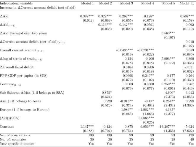
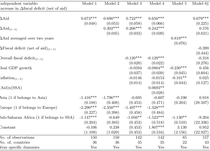
Table 1 reports the programmed absorption of aid increase, whereas Table 2 reports the programmed spending of aid increase with various regression models. These sets of models are employed here to replicate the results of
the IEO (2007) with better dataset and improved estimation techniques. Al-though our preferred estimate is the Blundell-Bond GMM estimation (Model 6), we still used other models to check the robustness of our estimations. To capture the amount of smoothing, the lagged change in aid is included in the regression. Such control variables are appropriate to estimate the programmed widening of the current account deficit (or fiscal deficit), which is influenced by the use of the aid changes that were not absorbed (or spent) in the previous year and a positive coefficient of the lagged change in aid implies the smoothing of the aid inflows.
The regressions in Table 1 suggest that immediate absorption of aid inflow is 59 percent, whereas Table 2 shows that the immediate spending of aid inflow is 68 percent. Such findings contradict the IEO (2007) which found that approximately 27 percent of aid increase is spent and some 64 percent is absorbed immediately. However, our results are in line with the conclusion by Aiyar and Ruthbah (2008), in which they found that spending is higher than absorption. Controlling for other factors, our results remain stable. Our regressions also provide evidence of smoothing in both absorption and spending estimations. Model 3 of the absorption regression shows that 26 percent of the expected increase in aid is programmed to be absorbed in the first programming year, whereas the coefficient on the lagged increase in aid indicates that 14 percent of the past increase in aid is to be absorbed in the programming year. Similarly, Model 3 of the spending regression shows that 72 percent of the aid increase is programmed to be spent immediately and about 27 percent is programmed to be utilized in the following year.
[Table 1 and 2 about here]
Controlling for other variables suggests that concerns for fiscal instability and reserve inadequacy can weaken the programmed absorption and spend-ing of aid. Likewise, we find evidence of difference in spendspend-ing and ab-sorption for countries of Sub-Saharan Africa (SSA). The coefficient of the interaction term between SSA and aid increase suggests that spending and absorption is significantly higher for the countries that belong to SSA areas.
An alternative method for examining the smoothing of the use of aid is to use the cumulative increase of the programmed fiscal deficits (or current account deficit) over a two-year period and the projected increase in aid
over the same period. In the case of spending, the regression confirms that the spending of aid over a two-year period is more than 81 percent (Table 2, Model 5). This finding is quite important since it shows that fiscal deficits are programmed for a time horizon that is longer than one year. Similarly, for absorption the regression indicates that the absorption of aid over a two-year period is about 56 percent (Table 1, Model 5).
In our preferred regression for both spending and absorption, we find weak evidence for the smoothing of aid use. One reason for this finding could be the use of only positive changes in aid in the regressions, which provide partial and quite plausibly misleading results of the regressions. In the next subsection, we will relax such restrictions.
6.2 Absorption, Spending and Smoothing of Aid
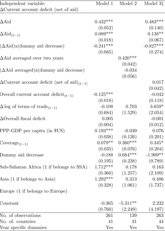
Restricting the sample for only positive changes in aid provides a partial and misleading scenario of the use of aid. In the case of aid volatility, consideration of the treatment of both aid increase and decrease should be included to correctly understand the use of aid. Aid volatility elicits the question as to weather the programmed response to changes in aid is symmetric. To answer this question, we looked at both directions of the changes in aid inflows.
[Table 3 and 4 about here]
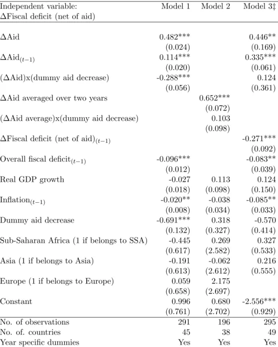
Table 3 and Table 4 present the regression for absorption and spending respectively. Model 3 of the absorption regression suggests the smoothing of the programmed use of aid, where approximately 48 percent of aid increase is programmed to be spent instantly and approximately 13 percent of the past increase in aid is to be absorbed in the current programming year. This makes the eventual absorption ratio about 62 percent. Similarly, Model 3 of the spending regression shows evidence of smoothing of aid, as some 44 percent of aid increase is programmed to be used immediately, whereas roughly 33 percent of the past increase in aid is to be spent in the current programming year, making the eventual spending ratio 78 percent.
To control for the symmetric use of aid, we used an interaction term between the expected change in aid with a dummy variable that takes a value of one
if the expected change in aid is negative. Our regressions indicate that in the case of absorption, the aid decreases are treated asymmetrically to aid increases since the interaction term is significant and negative. The negative sign of the interaction term suggests that if aid is expected to fall over the course of the program, the programmed contraction of the current account deficit net of aid is smaller than the expansion that is permitted during aid increments. However, in the case of spending, such asymmetry does not exist. Furthermore, in the two-year horizon model (Model 2 in Table 3 and 4) we did not find any evidence of asymmetric use of aid. Findings of symmetric treatment of aid increases and decreases in the longer policy horizon could be driven by the expected stability of future aid flows.
In spending regressions, we found evidence that higher past overall fiscal deficit decreases the programmed change in fiscal deficit, and the significant coefficient of the lagged change in the fiscal deficit indicates the importance of stabilizing the deficit over time. Similarly, inflation has a considerable effect on the programmed change of fiscal deficit net of aid. In spending equations, we found significant association of reserve coverage and terms of trade with the change in the current account deficit net of aid, where both of these variables widen the programmed current account deficit.
6.3 Actual Absorption, Spending and Smoothing of Aid
Tables 5 and 6 report the various models used to estimate the absorption, spending and smoothing of the aid use by employing the actual rather than the programmed data of spending and absorption. This analysis will help in understanding the behavior of actual spending and absorption of aid compared with the programmed spending and absorption. The result for absorption (Model 8 in Table 5) suggests that actual absorption of the aid is about 28 percent with no evidence of smoothing of aid. This absorption rate is lower than the estimated programmed absorption found in previous subsections.
[Table 5 and 6 about here]
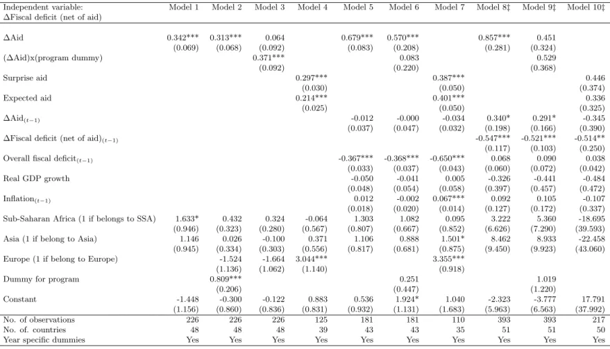
The result of the actual spending of same year use of aid is about 86 percent with marginal significant evidence of smoothing of aid over the years. The
eventual spending ratio of actual spending becomes more than 100 percent, which is consistent with the findings of Aiyar and Ruthbah (2008). One rea-son for these findings could be the certain aid-financed capital expenditures that might create a need for additional expenditures in each consecutive period.8 However, our findings of absorption are completely opposite to the findings of Aiyar and Ruthbah (2008) but are in line with the findings Berg et al. (2007), which indicate that aid can be sometimes be spent but not absorbed.
To understand the influence of the PRGF program on countries’ actual spending and absorption, we introduced an interaction term between aid and a dummy variable that is equal to one in those years the country is under a PRGF program. Our results suggest that the presence of a PRGF program does not seem to influence the actual spending and absorption of aid (row two of Model 9 in Tables 5 and 6). Furthermore, we control for the aid surprise, which is defined as the increments in aid that were not predicted during the programming period. Our preferred estimations (Model 10 of Tables 5 and 6) could not find any significant difference in the spending and absorption pattern of aid in case of aid surprise. Similarly, fiscal consolidation and reserve adequacy seems to have no significant impact on the actual spending and absorption of aid.
Finally, to realize the relationship between actual and program aid, we em-ployed Figures 1 and 2. The pictures suggest that generally IMF programs have a tendency to understate program aid inflows in case the level of aid is below average. However, the situation tends to reverse when the level of aid is higher than average. In this case, the programmed aid inflows are over-stated compared with the actual inflows of aid. This observation remains true for both the fiscal and BOP data.
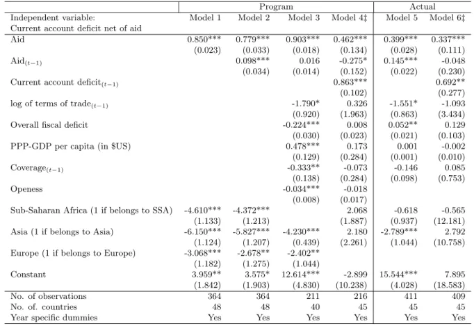
6.4 Absorption, Spending and Smoothing using levels of Aid
Tables 7 and 8 represent the estimations of spending and absorption of aid using levels of data (as a percentage of GDP) rather than the differences. These estimations are done as a robustness check to our previous
estima-8
For example, an aid-funded hospital might require perennial government expenditure on nurses and doctors, or a road may require repeated maintenance and repair costs.
tions. By using the actual and programmed data for levels of aid flows, the regression coefficients measure the fraction of aid inflow that is absorbed and spent over time.
Once again, our preferred models are Models 4 and 6 in both tables which employed the Blundell and Bond GMM estimations otherwise known as Sys-tem GMM techniques. The estimated programmed absorption is approxi-mately 46 percent in contrast with estimated actual absorption of about 34 percent. Coherent with the earlier estimations of this study, the estimated actual absorption is found to be lower than the programmed absorption. Model 6 of Table 7 also reveals that past current account deficit has sig-nificant positive association with the programmed year’s current account deficit net of aid, showing the persistent nature of the deficit in the balance of payments.
[Table 7 and 8 about here]
The estimated programmed spending is approximately 74 percent, whereas actual spending is some 97 percent. Consistent with the findings of the previous subsection, we find that actual spending is higher than the pro-grammed spending with evidence of smoothing of actual aid over time. The long-run spending is estimated to be higher than 100 percent, which makes the analysis coherent with the findings of earlier sub-sections. Furthermore, we found evidence that higher past overall fiscal deficit decreases the actual fiscal deficit of the program year.
7
Conclusion
Improving on Dudine et al. (2008), this study utilizes Blundell and Bond’s System GMM estimator to provide consistent estimates of the programmed absorption and spending of aid. However, the finding of the study should be received with caution as the estimations may have suffered due to the complexities of the issues and caveats resulting from the unavailability of data and the presence of outliers for important variables over the period we examined.
permit countries to utilize all increases in aid within a few years, demon-strating smoothed use of aid inflows over time. In addition, our result reveals that spending is higher than absorption in both the long-run and short-run use of aid and shows evidence of the injection of liquidity into the domes-tic economies of developing countries. Furthermore, the study finds that the long-run spending exceeds the injected increase of aid inflows in the economy. In contrast, we find weak evidence of profound influence of other control variables on the spending and absorption of aid. Finally, the study finds that the presence of a PRGF-supported program does not influence the actual absorption or spending of aid.
We suggest the following policy implications as a result of this study. Since macroeconomic considerations appear to have no influence over aid commit-ments and disbursecommit-ments, aid agencies should take account of the macroeco-nomic stability of an economy, as aid is found to have significant associations with balance of payments and national income accounting. Aid is some-times received as non-fungible project assistance, which raises government expenditure. Aid agencies should be cognisant of this type of assistance, as governments may need to cut necessary consumptions to finance aid-funded projects or may need to finance the expenditure from domestic borrowing. Aid volatility is also a concern for recipient countries which leads govern-ments to delay the immediate use of aid incregovern-ments. Such volatility should be reduced to improve the immediate use of aid.
References
Acemoglu, D., Johnson, S. and Robinson, J. (2001), ‘The colonial origins of comparative development: An empirical investigation’, The American Economic Review 91(5), 1369–1401.
Aiyar, S., Berg, A. and Hussain, M. (2005), ‘The macroeconomic challenge of more aid’,Finance and Development42(3), 2831.
Aiyar, S. S. and Ruthbah, U. H. (2008), ‘Where did all the aid go? an empirical analysis of absorption and spending’, SSRN eLibrary.
Monte carlo evidence and an application to employment equations’, The Review of Economic Studies 58(2), 277–297.
Aslam, A. and Kim, J. (2007), ‘Aid volatility and precautionary saving’.
Baum, C. (2006),An introduction to modern econometrics using Stata, Stata Corp.
Berg, A., Aiyar, S., Hussain, M., Roache, S., Mirzoev, T. and Mahone, A. (2005), ‘The macroeconomics of managing increased aid inflows’,IMF Occasional Paper .
Berg, A., Aiyar, S., Hussain, M., Roache, S., Mirzoev, T. and Mahone, A. (2007), ‘The macroeconomics of scaling up aid. lessons from recent experience’,IMF Occasional Paper No. 253 .
Blundell, R. and Bond, S. (1998), ‘Initial conditions and moment restrictions in dynamic panel data models’, Journal of Econometrics87(1), 115–143.
De Hoyos, R. and Sarafidis, V. (2006), ‘Testing for cross-sectional depen-dence in panel-data models’, Stata Journal6(4), 482.
Dudine, P., Berndt, M., Shonchoy, A. and Martijn, J. K. (2008), ‘The spend-ing and absorption of aid in PRGF supported programs’, IMF working Paper WP/08/237 .
Foster, M. and Killick, T. (2006), ‘What would doubling aid do for macroe-conomic management in Africa’, ODI Briefing Paper. London: ODI.
Frees, E. (1995), ‘Assessing cross-sectional correlation in panel data’, Jour-nal of econometrics69(2), 393–414.
Frees, E. (2004),Longitudinal and panel data: analysis and applications in the social sciences, Cambridge Univ Pr.
Friedman, M. (1937), ‘The use of ranks to avoid the assumption of normality implicit in the analysis of variance’, Journal of the American Statistical Association 32(200), 675–701.
Hansen, H. and Headey, D. (2009), ‘The short-run macroeconomic impact of foreign aid to small states: An agnostic time series analysis’, IFPRI discussion papers.
IEO (2007), ‘An Evaluation of the IMF and Aid to Sub-Saharan Africa’,
Independent Evaluation Office of the IMF, Evaluation report .
Nickell, S. (1981), ‘Biases in dynamic models with fixed effects’, Economet-rica 49(6), 1417–1426.
Pesaran, M. H. (2004), ‘General diagnostic tests for cross section dependence in panels’,SSRN eLibrary .
Putman, R. (1993), ‘Making democracy work’,Civic Traditions in Modern Italy .
Roodman, D. (2006), ‘How to do Xtabond2: An Introduction to Difference and System GMM in Stata’, SSRN eLibrary.
A
Appendix: The Model
Extending from Dudine et al. (2008), this framework proposes a simple model under which the spending and absorption equations in differences are compatible with the same equations in levels (and vice-versa).
Because the equation in difference considers the difference between the pro-grammed and the actual (lagged) level of variables, whereas the equation in level considers only the programmed level of variables, any model that attempts to make these two equations compatible must include, implicitly or explicitly, both an equation that explains the actual values of the vari-ables, and an equation that explains how expectations about the exogenous variables are formed.
The model proposed in this note allows coherency between the programming equation and the equation that explains the actual. Also, this model allows maintaining a richer description of spending and absorption, which includes the possibility of smoothing and the serial dependence of the endogenous variable to its lagged values.
Lets denote Yi,tp as the programmed level of the endogenous variable for countryi at time t (which is uniquely ranked and based on the date when the document was published). Note the endogenous variables are current account deficit net of aid or the fiscal deficit net of aid, in percent of GDP. Let Yi,te be the expected level and Yi,t be the actual level of such variable
for countryifor att. Similarly, Xi,tp , Xe
i,t and Xi,t are respectively the
pro-grammed, expected and actual level of aid for countryiat timet.Finally, let
Zi,t be a vector of explanatory variables and ui,t a zero-mean independent
and identically distributed error term. We introduce µi as the country
spe-cific time invariant effect. Thus the equations in levels for the programme can be expressed as:
Yi,tp =β0+β1Xi,tp +β2Xi,t−1+β3Zi,t−1+θYi,t−1+µi+ui,t. (17)
Assume that the actual level of the endogenous variable is described by the following model:
Yi,t=α0+α1Xi,t+α2Xi,t−1+α3Zi,t+λYi,t−1+µi+εi,t (18)
whereεi,tis a zero-mean independent and identically distributed error term.
Note when an IMF program is designed, the realization of εi,t, the actual
level of aid Xi,t and the actual level of the exogenous variables Zi,t are not
known. Hence programmed and expected values are used which makes the above equation as
E[Yi,t] =Yi,te =α0+α1Xi,te +α2Xi,t−1+α3Zi,te +λYi,t−1+µi (19)
whereE[εi,t] = 0.Assume that the programmed level of aid is exogenously
determined whereas the expectations about the level of the exogenous vari-ables are based on the past realization of these varivari-ables.9 Lets use the following equation:
Zi,te =ϕ+ρZi,t−1+ψi,t (20)
where ψi,t is a zero mean error term. If we plug equation 20 into 19 and
rearrange the terms, we obtain
Yi,te =α0+α3ϕ+α1Xi,te +α2Xi,t−1+α3ρZi,t−1+λYi,t−1+µi+α3ψi,t. (21)
Which is our equation in levels (equation 17) provided thatβ0 =α0+α3ϕ,
β1 =α1, β2=α2, β3 =α3ρ, θ=λand ui,t=α3ψi,t.
To obtain the equations in differences and purging the country specific fixed effect, we first use equation 18 to obtainYi,t−1.Then we subtract theYi,t−1
from the both side of the equation 21 to obtain
Yi,te −Yi,t−1 = α3ϕ+α1(Xi,te −Xi,t−1) +α2(Xi,t−1−Xi,t−2)
−α3(ρ−1)Zi,t−1+λ(Yi,t−1−Yi,t−2) +α3ψi,t−εi,t−(22)1.
9This is fairly sensible assumption since creditors’ aid commitments are generally
Hence, re-parameterizing the above equation, we can rewrite as
Yi,te −Yi,t−1 = γ0+γ1(Xi,te −Xi,t−1) +γ2(Xi,t−1−Xi,t−2)
+γ3Zi,t−1+δ(Yi,t−1−Yi,t−2) +ωi,t. (23)
Here γ0 = α3ϕ, γ1 = α1, γ2 = α2, γ3 = −α3(ρ−1), δ = λ and ωi,t =
α3ψi,t−εi,t−1.
This model allows to identify possible estimation problems. For instance, from ωi,t =α3ψi,t−εi,t−1, we can see that the error term of the equation
in difference is correlated with one of the regressors, namelyYi,t−1−Yi,t−2
which is corrected by using dynamic panel data estimation techniques in the regression estimation.
B
Appendix: Estimation Results
Figure 1: Actual and programmed aid inflows in the same year (BOP cal-culations)
Figure 2: Actual and programmed aid inflows in the same year (Fiscal calculations)
Table 1: Regression result for the absorption of aid increase, unbalanced panel (1999-2009).
Independent variable: Model 1 Model 2 Model 3 Model 4 Model 5 Model 6‡
Increase in ∆Current account deficit (net of aid)
∆Aid 0.392*** 0.322*** 0.262*** 0.128* 0.587*** (0.043) (0.063) (0.055) (0.073) (0.158) ∆Aid(t−1) 0.113*** 0.142*** 0.0591 0.092
(0.033) (0.029) (0.038) (0.110) ∆Aid averaged over two years 0.563***
(0.107)
∆Current account deficit (net of aid)(t−1) 0.010
(0.122) Overall current account(t−1) -0.0485*** -0.0731*** 0.053
(0.019) (0.022) (0.080) ∆ log of terms of trade(t−1) 0.124 -0.200 5.993*** 3.390
(0.878) (0.948) (2.172) (5.436) ∆Overall fiscal deficit 0.0184 0.0206 -0.011 (0.016) (0.018) (0.032) PPP-GDP per capita (in $US) 0.0698 0.249** 0.177 0.294 (0.072) (0.102) (0.110) (0.439) Coverage(t−1) 0.003 0.0300 0.250*** 0.267
(0.076) (0.077) (0.091) (0.449) Sub-Saharan Africa (1 if belongs to SSA) 0.875* 4.600* 3.913 (0.524) (2.373) (5.053) Asia (1 if belongs to Asia) 0.220 -0.913** -0.477 6.254** 3.298 (0.570) (0.374) (0.404) (2.434) (4.300) Europe (1 if belongs to Europe) -1.986** -2.982*** 4.135*
(0.865) (1.065) (2.377) (Aid)x(SSA) 0.0868*** (0.025) Constant 1.147*** -0.424 0.875 6.956*** -13.287*** -5.624 (0.188) (0.704) (0.754) (1.355) (7.622) No. of observations 130 130 99 99 93 128 No. of. countries 30 30 25 25 28 40 Year specific dummies Yes Yes Yes Yes Yes Yes Notes: Values in the parentheses are the reported standard errors of the estimation. Significance code: ***1%,
**5%, *10%. In model 1 to 4, the sample is restricted to observations where 0<∆Aid <10,−10<∆Current account deficit (net of aid)(t−1)<10. In model 5, the sample is restricted where 0 <∆Aid <10 and−20<
∆Current account deficit (net of aid)(t−1)<20. ‡Dynamic panel data estimations where the Hansen test for over
Table 2: Regression result for the spending of aid increase, unbalanced panel (1999-2009).
Independent variable: Model 1 Model 2 Model 3 Model 4 Model 5 Model 6‡
Increase in ∆fiscal deficit (net of aid)
∆Aid 0.673*** 0.690*** 0.722*** 0.650*** 0.679***
(0.048) (0.053) (0.058) (0.066) (0.225)
∆Aid(t−1) 0.302*** 0.266*** 0.242*** 0.576
(0.035) (0.033) (0.039) (0.621)
∆Aid averaged over two years 0.819***
(0.076)
∆Fiscal deficit (net of aid)(t−1) -0.399
(0.444)
Overall fiscal deficit(t−1) -0.120*** -0.129*** -0.318
(0.020) (0.022) (0.276) Real GDP growth -0.0594 -0.0804** -0.230*** 0.456 (0.037) (0.039) (0.045) (0.604) Inflation(t−1) -0.0146 -0.0153 -0.101** 0.025 (0.014) (0.014) (0.044) (0.127) (Aid)x(SSA) 0.0693** (0.028)
Asia (1 if belongs to Asia) -1.416*** -1.796*** -0.695 -0.607 -0.190 0.918
(0.188) (0.408) (0.453) (0.471) (0.204) (28.507)
Europe (1 if belongs to Europe) -2.290*** -2.350*** -1.497*** -1.328***
(0.227) (0.398) (0.458) (0.484)
Sub-Saharan Africa (1 if belongs to SSA) -1.147*** -0.649 -1.056** -1.523*** -1.130** -9.204
(0.204) (0.383) (0.453) (0.518) (0.510) (22.336)
Constant -0.106 0.238 (0.453) 1.807*** 3.130 0.952
(1.109) (1.029) (0.453) (0.534) (2.156) (22.927)
No. of observations 150 150 142 142 85 157
No. of. countries 36 36 35 35 22 43
Year specific dummies Yes Yes Yes Yes Yes Yes
Notes: Values in the parentheses are the reported standard errors of the estimation. Significance code: ***1%, **5%, *10%. In model 1 to 4, sample is restricted to observations where 0 < ∆Aid < 10, ∆Aid(t−1)> −10,
−10 < ∆Fiscal deficit (net of aid)(t−1)< 10 and Overall fiscal deficit(t−1)< 20. In model 5, the sample is
restricted to observations where 0<∆Aid <10 and−20<∆Fiscal deficit (net of aid)(t−1)<20. ‡Dynamic panel
Table 3: Regression result for the treatment of increase and decrease in aid (absorption), unbalanced panel (1999-2009).
Independent variable: Model 1 Model 2 Model 3‡
∆Current account deficit (net of aid)
∆Aid 0.432*** 0.483***
(0.052) (0.140)
∆Aid(t−1) 0.089*** 0.138**
(0.018) (0.067) (∆Aid)x(dummy aid decrease) -0.241*** -0.827*** (0.085) (0.274) ∆Aid averaged over two years 0.420***
(0.042) (∆Aid averaged)x(dummy aid decrease) -0.034 (0.056)
∆Current account deficit (net of aid)(t−1) 0.017
(0.042) Overall current account deficit(t−1) -0.125*** -0.042
(0.018) (0.118) ∆ log of terms of trade(t−1) -0.108 0.703 3.659*
(0.684) (1.529) (2.054) ∆Overall fiscal deficit 0.005 -0.001 (0.004) (0.012) PPP-GDP per capita (in $US) 0.193*** -0.039 0.076 (0.038) (0.126) (0.201) Coverage(t−1) 0.079** 0.360*** 0.345*
(0.035) (0.076) (0.204) Dummy aid decrease -0.188 0.684*** -1.909** (0.195) (0.238) (0.789) Sub-Saharan Africa (1 if belongs to SSA) 1.712*** 0.178 0.163 (0.360) (1.257) (2.109) Asia (1 if belongs to Asia) 1.292*** 0.313 0.486 (0.328) (1.061) (1.737) Europe (1 if belongs to Europe)
Constant -0.365 -5.311** 2.232
(0.760) (2.249) (4.197)
No. of observations 261 139 263
No. of. countries 41 31 44
Year specific dummies Yes Yes Yes
Notes: Values in the parentheses are the reported standard errors of the estimation. Sig-nificance code: ***1%, **5%, *10%. In model 1 to 2, sample is restricted to observations where−10<∆Aid <10,−10<∆Current account deficit (net of aid)(t−1)<10. ‡Dynamic
panel data estimations where the Hansen test for over identifying restriction is rejected and no evidence for AR(1) and AR(2) process after the estimation.
Table 4: Regression result for the treatment of increase and decrease in aid (spending), unbalanced panel (1999-2009).
Independent variable: Model 1 Model 2 Model 3‡
∆Fiscal deficit (net of aid)
∆Aid 0.482*** 0.446**
(0.024) (0.169)
∆Aid(t−1) 0.114*** 0.335***
(0.020) (0.061) (∆Aid)x(dummy aid decrease) -0.288*** 0.124 (0.056) (0.361) ∆Aid averaged over two years 0.652***
(0.072) (∆Aid average)x(dummy aid decrease) 0.103 (0.098)
∆Fiscal deficit (net of aid)(t−1) -0.271***
(0.092) Overall fiscal deficit(t−1) -0.096*** -0.083**
(0.012) (0.039) Real GDP growth -0.027 0.113 0.124 (0.018) (0.098) (0.150) Inflation(t−1) -0.020** -0.038 -0.085**
(0.008) (0.034) (0.033) Dummy aid decrease -0.691*** 0.318 -0.570 (0.132) (0.327) (0.414) Sub-Saharan Africa (1 if belongs to SSA) -0.445 0.269 0.327 (0.617) (2.582) (0.533) Asia (1 if belongs to Asia) -0.191 -0.062 0.216 (0.613) (2.612) (0.555) Europe (1 if belongs to Europe) 0.059 2.175
(0.658) (2.697)
Constant 0.996 0.680 -2.556***
(0.761) (2.702) (0.929)
No. of observations 291 196 295
No. of. countries 45 38 49
Year specific dummies Yes Yes Yes
Notes: Values in the parentheses are the reported standard errors of the estimation. Sig-nificance code: ***1%, **5%, *10%. In model 1 and 3, sample is restricted to observations where−10<∆Aid <10, ∆Aid(t−1)>−20 and−10<∆Fiscal deficit (net of aid)(t−1)<10.
In model 2, the sample is restricted to observations where−10<∆Aid < 10. ‡Dynamic panel data estimations where the Hansen test for over identifying restriction is rejected and no evidence for AR(1) and AR(2) process after the estimation.
Table 5: Regression result for the actual absorption of aid, unbalanced panel (1999-2009).
Independent variable: Model 1 Model 2 Model 3 Model 4 Model 5 Model 6 Model 7 Model 8‡ Model 9‡ Model 10‡
∆Current account deficit (net of aid)
∆Aid 0.129** 0.146** 0.124 0.047 -0.008 0.278*** 0.643 (0.057) (0.061) (0.111) (0.083) (0.184) (0.084) (0.453) (∆aid)x(program dummy) 0.042 0.077 -0.456 (0.119) (0.213) (0.971) Surprise aid 0.068 -0.011 0.284 (0.060) (0.060) (0.224) Expected aid 0.117*** 0.237*** 0.366 (0.017) (0.021) (0.459) ∆Aid(t−1) -0.160*** -0.162*** -0.007 0.121 0.252** 0.039 (0.044) (0.046) (0.021) (0.097) (0.119) (0.605) ∆Current account deficit (net of aid)(t−1) -0.408** -0.467** -0.405
(0.160) (0.210) (0.667) Overall current account deficit(t−1) -0.152*** -0.176*** -0.173*** -0.383 -0.573 -0.320
(0.040) (0.038) (0.035) (0.387) (0.490) (0.836) ∆ log of terms of trade(t−1) -3.309* -2.945* -4.623*** -1.667 -1.849 15.985
(1.730) (1.720) (1.197) (16.187) (14.165) (27.103) ∆Overall fiscal deficit 0.091*** 0.090*** 0.101*** 0.105 0.111 0.058
(0.029) (0.029) (0.019) (0.074) (0.098) (0.121) PPP-GDP per capita (in $US) -0.001 -0.002 0.005*** 0.004 0.008 0.019 (0.001) (0.001) (0.001) (0.012) (0.023) (0.046) Coverage(t−1) -0.164* -0.047 -0.097 -0.735 -0.717 -2.085
(0.088) (0.099) (0.129) (0.937) (1.399) (3.826) Sub-Saharan Africa (1 if belongs to SSA) 1.023 1.042 -1.350*** 2.600 -1.331 -1.725** 0.633 4.513 5.455 3.155 (2.891) (2.941) (0.454) (2.242) (0.883) (0.812) (0.739) (10.499) (16.476) (24.095) Asia (i if belongs to Asia) 1.182 1.135 -1.080** 2.973 -2.488** -2.458** -1.255 -2.966 -1.661 0.432 (2.904) (2.960) (0.519) (2.247) (0.970) (0.965) (0.838) (15.018) (19.476) (16.931) Europe (1 if belongs to Europe) -2.378 -4.348 -3.929 -3.614
(2.892) (3.701) (3.819) (2.273)
Dummy for program 0.168 0.742 -11.551
(0.251) (0.766) (8.278)
Constant -0.769 -0.719 9.156*** -4.937** 3.082 3.833* -1.669 1.945 2.509 -5.990 (3.031) (3.077) (1.897) (2.378) (2.910) (2.049) (1.243) (13.722) (22.186) (39.888) No. of observations 198 198 198 98 142 142 82 367 367 202 No. of. countries 44 44 44 31 35 35 27 45 45 45 Year specific dummies Yes Yes Yes Yes Yes Yes Yes Yes Yes Yes Notes: Values in the parentheses are the reported standard errors of the estimation. Significance code: ***1%, **5%, *10%. In model 1 to 7, the
sample is restricted to observations where 0<∆Aid <10.‡Dynamic panel data estimations where the Hansen test for over identifying restriction
Table 6: Regression result for the actual spending of aid, unbalanced panel (1999-2009).
Independent variable: Model 1 Model 2 Model 3 Model 4 Model 5 Model 6 Model 7 Model 8‡ Model 9‡ Model 10‡
∆Fiscal deficit (net of aid)
∆Aid 0.342*** 0.313*** 0.064 0.679*** 0.570*** 0.857*** 0.451 (0.069) (0.068) (0.092) (0.083) (0.208) (0.281) (0.324) (∆Aid)x(program dummy) 0.371*** 0.083 0.529 (0.092) (0.220) (0.368) Surprise aid 0.297*** 0.387*** 0.446 (0.030) (0.050) (0.374) Expected aid 0.214*** 0.401*** 0.336 (0.025) (0.050) (0.325) ∆Aid(t−1) -0.012 -0.000 -0.034 0.340* 0.291* -0.345 (0.037) (0.047) (0.032) (0.198) (0.166) (0.390) ∆Fiscal deficit (net of aid)(t−1) -0.547*** -0.521*** -0.514**
(0.117) (0.103) (0.250) Overall fiscal deficit(t−1) -0.367*** -0.368*** -0.650*** 0.068 0.090 0.038
(0.033) (0.037) (0.043) (0.060) (0.072) (0.042) Real GDP growth -0.050 -0.041 0.005 -0.326 -0.441 -0.484 (0.048) (0.054) (0.058) (0.397) (0.457) (0.472) Inflation(t−1) 0.012 -0.002 0.067*** 0.092 0.105 -0.107
(0.018) (0.020) (0.014) (0.127) (0.172) (0.337) Sub-Saharan Africa (1 if belongs to SSA) 1.633* 0.432 0.324 -0.064 1.303 1.082 0.095 3.222 5.360 -18.695 (0.946) (0.323) (0.280) (0.567) (0.807) (0.667) (0.852) (6.626) (7.290) (39.593) Asia (1 if belong to Asia) 1.146 0.026 -0.100 0.371 1.106 0.888 1.501* 8.462 8.933 -22.458 (0.945) (0.334) (0.303) (0.556) (0.817) (0.681) (0.875) (9.450) (9.923) (43.060) Europe (1 if belong to Europe) -1.524 -1.664 3.044*** 3.355***
(1.136) (1.062) (1.140) (0.918)
Dummy for program 0.809*** 0.251 1.019
(0.206) (0.447) (1.220)
Constant -1.448 -0.300 -0.122 0.883 0.536 1.924* 1.040 -2.323 -3.777 17.791 (1.156) (0.860) (0.836) (0.831) (0.932) (1.131) (1.683) (5.963) (6.563) (37.992) No. of observations 226 226 226 125 181 181 110 393 393 217 No. of. countries 48 48 48 39 43 43 35 51 51 50 Year specific dummies Yes Yes Yes Yes Yes Yes Yes Yes Yes Yes Notes: Values in the parentheses are the reported standard errors of the estimation. Significance code: ***1%, **5%, *10%. In model 1 to 7, the
Table 7: Regression result for the absorption using level of aid inflows, unbalanced panel (1999-2009).
Program Actual
Independent variable: Model 1 Model 2 Model 3 Model 4‡ Model 5 Model 6‡ Current account deficit net of aid
Aid 0.850*** 0.779*** 0.903*** 0.462*** 0.399*** 0.337*** (0.023) (0.033) (0.018) (0.134) (0.028) (0.111) Aid(t−1) 0.098*** 0.016 -0.275* 0.145*** -0.048
(0.034) (0.014) (0.152) (0.022) (0.230) Current account deficit(t−1) 0.863*** 0.692**
(0.102) (0.277) log of terms of trade(t−1) -1.790* 0.326 -1.551* -1.093
(0.920) (1.963) (0.863) (3.434) Overall fiscal deficit -0.224*** 0.008 0.052** 0.129 (0.030) (0.023) (0.021) (0.103) PPP-GDP per capita (in $US) 0.478*** 0.173 0.001 -0.002 (0.129) (0.284) (0.001) (0.010)
Coverage(t−1) -0.333** -0.073 -0.146 0.085
(0.138) (0.284) (0.098) (0.753)
Openess -0.034*** -0.018
(0.008) (0.017)
Sub-Saharan Africa (1 if belongs to SSA) -4.610*** -4.372*** 2.068 -0.618 -0.565 (1.133) (1.213) (1.887) (0.937) (12.181) Asia (1 if belongs to Asia) -6.150*** -5.827*** -4.230*** 2.180 -2.789*** 2.792 (1.124) (1.207) (0.439) (2.261) (1.044) (10.758) Europe (1 if belongs to Europe) -3.068*** -2.678** -2.402**
(1.182) (1.275) (1.044)
Constant 3.959** 3.575* 12.614*** -2.899 15.544*** 7.895 (1.842) (1.903) (4.830) (10.238) (4.028) (18.583)
No. of observations 364 364 211 216 411 409
No. of. countries 48 48 40 45 45 45
Year specific dummies Yes Yes Yes Yes Yes Yes
Notes: Values in the parentheses are the reported standard errors of the estimation. Significance code: ***1%, **5%, *10%. In model 1 to 3 and 5, the sample is restricted to observations where Current account deficit<70. ‡Dynamic panel data estimations where the Hansen test for over identifying restriction is rejected and no evidence
Table 8: Regression result for the spending using level of aid inflows, unbalanced panel (1999-2009).
Program Actual
Independent variable: Model 1 Model 2 Model 3 Model 4‡ Model 5 Model 6‡ Fiscal deficit net of aid
Aid 0.867*** 0.761*** 0.744*** 0.736*** 0.726*** 0.967*** (0.019) (0.028) (0.026) (0.125) (0.028) (0.157) Aid(t−1) 0.147*** 0.150*** -0.030 0.211*** 0.191**
(0.023) (0.023) (0.080) (0.026) (0.075) Fiscal deficit (net of aid)(t−1) 0.299*** -0.199***
(0.061) (0.062) Inflation(t−1) -0.027*** -0.018 -0.015** 0.058
(0.009) (0.039) (0.008) (0.107) Real GDP growth 0.078*** 0.386* 0.113*** -0.417 (0.026) (0.224) (0.032) (0.397) Sub-Saharan Africa (1 if belongs to SSA) -1.240*** -1.621*** -1.049* -3.070 -0.703** -5.487 (0.395) (0.394) (0.569) (1.980) (0.329) (9.475) Asia (1 if belongs to Asia) -0.627 -0.765* -0.211 0.092 0.263 -7.910 (0.423) (0.408) (0.572) (0.925) (0.282) (9.549) Europe (1 if belongs to Europe) -0.286 -0.416
(0.751) (0.710)
Constant 1.521* 1.865** 1.466 -3.342* -0.026 4.230 (0.836) (0.804) (1.053) (1.903) (0.638) (8.893)
No. of observations 337 337 317 321 417 434
No. of. countries 46 46 46 50 51 51
Year specific dummies Yes Yes Yes Yes Yes Yes
Notes: Values in the parentheses are the reported standard errors of the estimation. Significance code: ***1%, **5%, *10%. In model 1 to 4 and 5, the sample is restricted to observations where−20<Fiscal deficit<30 and −5<Aid inflows<30.. ‡Dynamic panel data estimations where the Hansen test for over identifying restriction is rejected and no evidence for AR(1) and AR(2) process after the estimation.
Source: International Monetary Fund Spending and Absorption data set 2008.
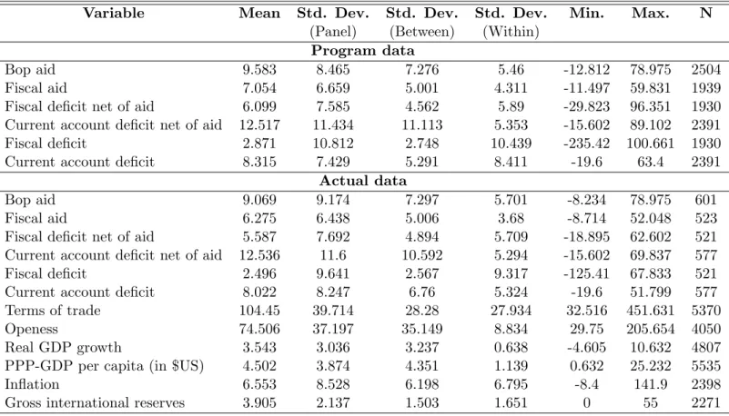
Table 9: Summary statistics
Variable Mean Std. Dev. Std. Dev. Std. Dev. Min. Max. N (Panel) (Between) (Within)
Program data
Bop aid 9.583 8.465 7.276 5.46 -12.812 78.975 2504 Fiscal aid 7.054 6.659 5.001 4.311 -11.497 59.831 1939 Fiscal deficit net of aid 6.099 7.585 4.562 5.89 -29.823 96.351 1930 Current account deficit net of aid 12.517 11.434 11.113 5.353 -15.602 89.102 2391 Fiscal deficit 2.871 10.812 2.748 10.439 -235.42 100.661 1930 Current account deficit 8.315 7.429 5.291 8.411 -19.6 63.4 2391
Actual data
Bop aid 9.069 9.174 7.297 5.701 -8.234 78.975 601 Fiscal aid 6.275 6.438 5.006 3.68 -8.714 52.048 523 Fiscal deficit net of aid 5.587 7.692 4.894 5.709 -18.895 62.602 521 Current account deficit net of aid 12.536 11.6 10.592 5.294 -15.602 69.837 577 Fiscal deficit 2.496 9.641 2.567 9.317 -125.41 67.833 521 Current account deficit 8.022 8.247 6.76 5.324 -19.6 51.799 577 Terms of trade 104.45 39.714 28.28 27.934 32.516 451.631 5370 Openess 74.506 37.197 35.149 8.834 29.75 205.654 4050 Real GDP growth 3.543 3.036 3.237 0.638 -4.605 10.632 4807 PPP-GDP per capita (in $US) 4.502 3.874 4.351 1.139 0.632 25.232 5535 Inflation 6.553 8.528 6.198 6.795 -8.4 141.9 2398 Gross international reserves 3.905 2.137 1.503 1.651 0 55 2271