Statistical Methods for Biodiversity Assessment

(1)

Full text document (pdf)

Copyright & reuse

Content in the Kent Academic Repository is made available for research purposes. Unless otherwise stated all content is protected by copyright and in the absence of an open licence (eg Creative Commons), permissions for further reuse of content should be sought from the publisher, author or other copyright holder.

Versions of research

The version in the Kent Academic Repository may differ from the final published version.

Users are advised to check http://kar.kent.ac.uk for the status of the paper. Users should always cite the published version of record.

Enquiries

For any further enquiries regarding the licence status of this document, please contact:

[email protected]

If you believe this document infringes copyright then please contact the KAR admin team with the take-down information provided at http://kar.kent.ac.uk/contact.html

Citation for published version

Kumphakarm, Ratchaneewan (2016) Statistical Methods for Biodiversity Assessment. Doctor

of Philosophy (PhD) thesis, University of Kent,.

DOI

Link to record in KAR

http://kar.kent.ac.uk/60557/

Document Version

(2)

Assessment

Ratchaneewan Kumphakarm

September 2016

A thesis submitted for the degree of

Doctor of Philosophy

School of Mathematics, Statistics and Actuarial Science

University of Kent

(3)

This thesis focuses on statistical methods for estimating the number of species which is a natural index for measuring biodiversity. Both parametric and nonparametric approaches are investigated for this problem. Species abun-dance models including homogeneous and heterogeneous model are explored for species richness estimation. Two new improvements to the Chao estimator are developed using the Good-Turing coverage formula.

Although the homogeneous abundance model is the simplest model, the species are collected with different probability in practice. This leads to overdispersed data, zero inflation and a heavy tail. The Poisson-Tweedie distribution, a mixed-Poisson distribution including many special cases such as the negative-binomial distribution, Poisson, Poisson inverse Gaussian, P´olya-Aeppli and so on, is explored for estimating the number of species. The weighted linear re-gression estimator based on the ratio of successive frequencies is applied to data generated from the Poisson-Tweedie distribution. There may be a prob-lem with sparse data which provides zero frequencies for species seen i times. This leads to the weighted linear regression not working. Then, a smoothing technique is considered for improving the performance of the weighted linear regression estimator. Both simulated data and some real data sets are used to study the performance of parametric and nonparametric estimators in this thesis.

(4)

Finally, the distribution of the number distinct species found in a sample is hard to compute. Many approximations including the Poisson, normal, COM-Poisson Binomial, Altham’s multiplicative and additive-binomial and P´olya distribution are used for approximating the distribution of distinct species. Under various abundance models, Altham’s multiplicative-binomial approxi-mation performs well. Building on other recent work, the maximum likelihood and the maximum pseudo-likelihood estimators are applied with Altham’s multiplicative-binomial approximation and compared with other estimators.

(5)

I would like to express my gratitude to my supervisor Professor Martin Ridout, for his patience, support and encouragement of my PhD study. He helped to guide me all the time for my research and writing my thesis. I sincerely ap-preciate Professor Martin Ridout as my supervisor. I could not have done this successfully without his guidance. My sincere thanks also goes to Dr.Alfred Kume who is my co-supervisor for his helpful advice and proof reading through-out my writing stages. It would not have been possible to complete the thesis without his guidance.

I am extremely grateful to my parents for encouragement all my life even dur-ing their illness. I would like to thank Claire Carter and Derek Baldwin for their helps and suggestions during four years of my PhD. I would also like to thank the School of Mathematics, Statistics and Actuarial Science at the University of Kent for providing the facilities for all the research students.

I am extremely grateful to the National Science and Technology Development Agency, Thai Government, for the scholarship to do my PhD in United King-dom. I would like to recognise my workplace, Maejo University, Thailand, for encouraging me to undertake the PhD. Finally, I would like to thank my friends, Bill, Kyle, Sam and Tita, for sharing their ideas, knowledge and time for coffee. Koi and Kung, my dear friends, who reminded me to do important things for the PhD.

(6)

Preface . . . i

Acknowledgment . . . iii

1 Introduction 1 1.1 Background . . . 1

1.2 Real data examples . . . 4

1.2.1 Malaysian butterfly data . . . 4

1.2.2 Pollutant data . . . 5

1.2.3 Christmas bird data . . . 5

1.2.4 Heroin users data . . . 6

1.2.5 Beetle data . . . 6

1.2.6 Tropical trees data . . . 7

1.3 Thesis Structure . . . 7

2 Species richness estimation 11 2.1 Introduction . . . 11

2.2 Sampling Models . . . 12

2.3 Species abundance model . . . 13

2.3.1 Deterministic models . . . 14

2.3.2 Random models . . . 15

2.3.3 Some numerical examples about species abundance models 17 2.4 Nonparametric approach . . . 20

2.4.1 Good-Turing estimator . . . 20

(7)

2.4.2 Chao1 Estimator . . . 22

2.4.3 iChao1 estimator . . . 24

2.4.4 Jackknife estimators . . . 27

2.4.5 Horvitz-Thompson estimator . . . 31

2.5 An alternative improvement to the Chao1 estimator . . . 32

2.6 Comparing previous model using simulation . . . 34

2.7 Simulation Study . . . 39

2.8 Real Data Examples . . . 49

2.9 Conclusion . . . 49

3 Estimating the number of species using maximum likelihood estimation 53 3.1 Introduction . . . 53

3.2 Mixed Poisson Models . . . 54

3.3 Maximum likelihood estimation based on zero-truncated Mixed-Poisson distribution . . . 60

3.4 Problems with maximum likelihood estimation . . . 65

4 Estimating the number of species using Poisson-Tweedie model 69 4.1 Introduction . . . 69

4.2 Poisson-Tweedie (PT) model for overdispersed data . . . 70

4.2.1 Tweedie distribution . . . 71

4.2.2 Poisson-Tweedie distribution . . . 73

4.2.3 Sub-families of the PT distribution . . . 74

4.2.4 Mean, Variance, Dispersion and Skewness . . . 75

4.2.5 The probability mass function . . . 76

4.2.6 The Reparametrization (µ, D, a) . . . 77

(8)

4.4 Weighted Linear Regression Analysis . . . 84

4.5 Simulation study and real data examples . . . 85

4.5.1 Simulation study . . . 85

4.5.2 Real data example . . . 95

5 Data Smoothing 101 5.1 Introduction . . . 101

5.2 Discrete kernel estimator . . . 102

5.2.1 Weight functions . . . 103

5.2.2 Other discrete kernels . . . 104

5.3 The performance measurement of the estimator . . . 106

5.4 Bandwidth Selection . . . 107

5.5 The np package for density estimation . . . 109

5.6 Simulation study . . . 109

6 New approximations for the number of observed species 122 6.1 Introduction . . . 122

6.2 Distribution of number of observed species . . . 124

6.3 The classical occupancy problem . . . 127

6.4 Approximation to the distribution of K . . . 129

6.4.1 Poisson Approximation . . . 130

6.4.2 Normal Approximation . . . 132

6.4.3 COM-Poisson-Binomial Approximation . . . 132

6.4.4 Altham’s multiplicative binomial Approximation . . . 134

6.4.5 Altham’s additive binomial Approximation . . . 135

6.4.6 P´olya distribution . . . 135

6.4.7 Choosing parameters for the approximating distribution 137 6.5 Example-birthday coincidences . . . 138

(9)

6.6 Simulation Study . . . 142

7 Estimating the number of unseen species using approximations to the distribution of seen species 157 7.1 Introduction . . . 157

7.2 Hidaka’s parametric method . . . 158

7.2.1 Evaluation of P(Kr|Mr, N,θ) . . . 159

7.2.2 Construction of the data sets D1, . . . , Dm . . . 161

7.3 Least squares estimator (LS) . . . 162

7.4 Measuring the accuracy of the MLE . . . 163

7.4.1 Likelihood function of species sampling . . . 163

7.4.2 Fisher information . . . 164

7.5 Simulation study . . . 168

8 Conclusion and Future work 178 8.1 Conclusion . . . 178

(10)

1.1 Frequency counts for Malaysian Butterfly Data (Fisher et al., 1943) . . . 5 1.2 Frequency counts for Pollutant Data (Janardan and Schaeffer,

1981) . . . 5 1.3 Frequency counts for the Christmas bird data at Fort Myers,

Florida, USA. (Chao and Bunge, 2002) . . . 5 1.4 Frequency counts for the heroin user data in Thailand (Lanumteang

and B¨ohning, 2011) . . . 6 1.5 Frequency counts for the beetle data collected from two sites in

southwestern Costa Rica (Janzen, 1973) . . . 6 1.6 Frequency counts for the tropical tree data observed from three

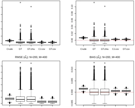
forest sites in northeastern Costa Rica (Norden et al., 2009) . . 7 2.1 Bias and RMSE of α_b1 (×10000) with 10000 times . . . 37

2.2 Bias and RMSE of α_b3 (×10000) with 10000 times . . . 38

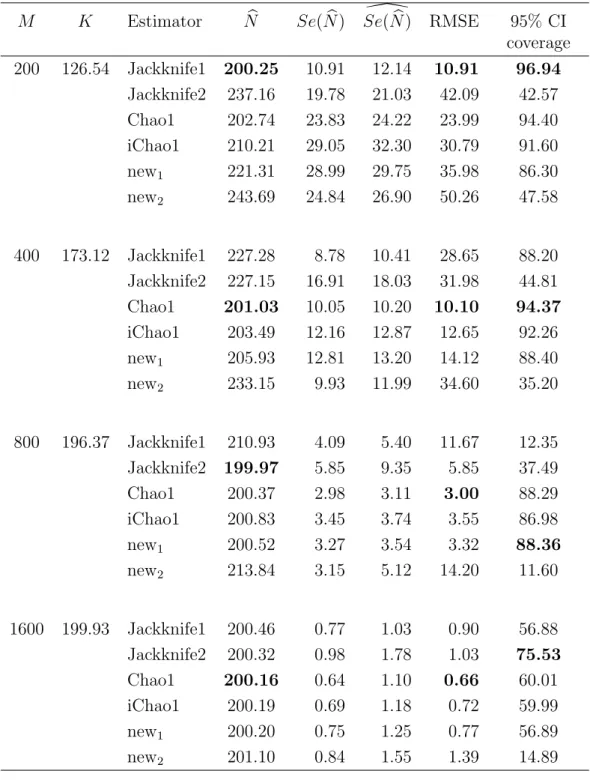
2.3 Comparison of the mean of species richness estimators based on the homogeneous model pi = 1/N with N = 200 and 10000

simulations. . . 43 2.4 Comparison of the mean of species richness estimators based on

the negative binomial (4, 0.04) model with N = 200 and 10000 simulations. . . 44

(11)

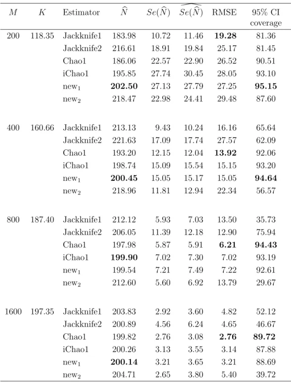
2.5 Comparison of the mean of species richness estimators based on the power decay model pi = c/i1.2 with N = 200 and 10000

simulations. . . 45 2.6 Comparison of the mean of species richness estimators based on

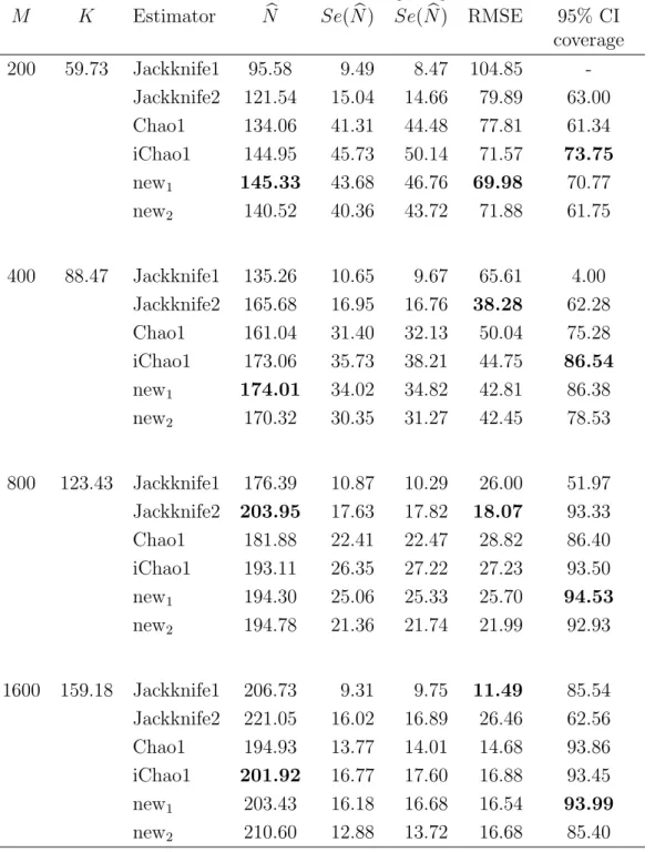
the log-normal(0,1) model with N = 200 and 10000 simulations. 46 2.7 Comparison of the mean of species richness estimators based on

the Zipf-Mandelbrot modelpi =c/(i−0.1), i= 1,2, . . . , N with

N = 200 and 10000 simulations. . . 47 2.8 Comparison of the mean of species richness estimators based on

the broken-stick model (or Dirichlet(1,1, . . . ,1)) with N = 200 and 10000 simulations. . . 48 2.9 Comparison of six estimators of total number for real data sets. 51 3.1 Estimated N, estimated standard error of N,Sec(Nb), 95%

con-fidence interval of N and AIC criterion. . . 64 4.1 Performance of NbW LR based on the PT distribution with N =

100, µ = 1, D = 1.1,1.25,1.5,2, a = ₋1,0,0.25,0.5,0.75,0.9 and 10000 simulations. . . 87 4.2 Performance of NbW LR based on the PT distribution with N =

1000, µ = 2, D = 1.1,1.25,1.5,2, a = ₋1,0,0.25,0.5,0.75,0.9 and 10000 simulations. . . 90

(12)

4.5 RMSE and bias of five estimators based on the PT distribution withN = 100µ= 1,D= 1.1,1.25,1.5,2,a =₋1,0,0.25,0.5,0.75,0.9 and 10000 simulations. . . 91 4.6 RMSE and bias of five estimators based on the PT distribution

withN = 100µ= 2,D= 1.1,1.25,1.5,2,a =₋1,0,0.25,0.5,0.75,0.9 and 10000 simulations. . . 92 4.7 RMSE and bias of five estimators based on the PT distribution

withN = 1000,µ= 1,D= 1.1,1.25,1.5,2,a =₋1,0,0.25,0.5,0.75,0.9 and 10000 simulations. . . 93 4.8 RMSE and bias of five estimators based on the PT distribution

withN = 1000,µ= 2,D= 1.1,1.25,1.5,2,a =₋1,0,0.25,0.5,0.75,0.9 and 10000 simulations. . . 94 4.9 Comparison of six estimators of total number for real data sets

and p-value from χ2 _{goodness of fit test for the WLR estimator. 97}

5.1 RMSE, bias, true standard error and estimated standard error for Nb based on the WLR estimator with nonsmoothing, the WLR with smoothing and the Chao1 estimator ;N = 100,1000,

µ= 1, D= 1.1.1.25.1.5.2, a= 0 using 1000 simulations. . . 114 5.2 RMSE, bias, true standard error and estimated standard error

for Nb based on the WLR estimator with nonsmoothing, the WLR with smoothing and the Chao1 estimator ;N = 100,1000,

µ= 2, D= 1.1.1.25.1.5.2, a= 0 using 1000 simulations. . . 115 5.3 RMSE, bias, true standard error and estimated standard error

for Nb based on the WLR estimator with nonsmoothing, the WLR with smoothing and the Chao1 estimator ;N = 100,1000,

(13)

5.4 RMSE, bias, true standard error and estimated standard error for Nb based on the WLR estimator with nonsmoothing, the WLR with smoothing and the Chao1 estimator ;N = 100,1000,

µ= 2, D= 1.1,1.25,1.5,2, a= 0.5 using 1000 simulations. . . . 118 6.1 Probability of birthday coincidences P(K < M) for the

occu-pancy problem when N = 365 . . . 141 6.2 Distance measures (_×105_), _d 2 = 1 2 P |p(x)₋p∗₍_x₎_| _and _d 3 =

max_|p(x)₋p∗₍_x₎_|_{, for Poisson(}_{N e}−M/N_{)), Poisson(}_N₍₁₋₁_/N₎M_),

Poisson(Var(X)), Normal, CMPB, Altham’s (MB and AB) and P´olya based on small N and M _≤100 with pi =

1 N. . . 147 6.3 Distance measures (_×105_), _d 2 = 1 2 P |p(x)₋p∗₍_x₎_| _and _d 3 =

Poisson(Var(K)), Normal, CMPB, Altham’s (MB and AB) and P´olya based on small N and M _≤100 with various unequal pi. 148

6.4 Distance measures (_×105_), _d 2 = 1 2 P |p(x)₋p∗₍_x₎_| _and _d 3 =

Poisson(Var(K)), Normal, CMPB, Altham’s (MB and AB) and P´olya based on large N and M (fixed M and N) with pi =

1 N. . 149 6.5 Distance measures (_×105_), _d 2 = 1 2 P |p(x)₋p∗₍_x₎_| _and _d 3 =

Poisson(Var(K)), Normal, CMPB, Altham’s (MB and AB) and P´olya based on large N and M (fixed M and N) with various unequal pi. . . 151 6.6 Distance measures (_×105_), _d 2 = 1 2 P |p(x)₋p∗₍_x₎_| _and _d 3 =

Poisson(Var(K)), Normal, CMPB, Altham’s (MB and AB) and P´olya based on very small and very large M

N with pi =

1

(14)

6.7 Distance measures (_×105_), _d 2 = 1 2 P |p(x)₋p∗₍_x₎_| _and _d 3 =

Poisson(Var(K)), Normal, CMPB, Altham’s (MB and AB) and P´olya based on very small and very large M

N with various

un-equal pi. . . 154

7.1 Number of times that convergence was achieved of optimization using various estimators based on the abundance data following the homogeneous model with repeated 100 times. . . 172 7.2 BIAS and RMSE ofNbusing the Chao1, iChao1, Good-Turing(GT),

Horviz-Tompson(HT), MLE with the PB and Altham distribu-tion (MLEpb and MLEal, MPLE with the PB (MLPEpb) and LS

(15)

2.1 Probability pi for distinct species i = 1,2, . . . , N, with N =

50 using different models, Zipf-Mandelbrot pi = 1/(i − 0.1),

negative binomial(4,0.04), broken-stick (or Dirichlet(1)), log-normal(0,1), power-decaypi = 1/i1.2and expo-decaypi = exp(−i).

17

2.2 Plot of rankedpi’s values for the Zipf model withN = 100,αin

the range [0.3,0.9] and broken-stick model with 20 simulations. 18 2.3 Plot of ranked pi’s values for the Zipf model with N = 100, α

in the range [0.3,0.9] and log-normal(0,1) model 20 simulations. 19 2.4 Plot of ranked pi’s values for the Zipf model with N = 100, α

in the range [0.2,0.8] and NB(4,0.04) model with 20 simulations. 19 2.5 Plot of ranked pi’s values for the Zipf model and expo-decay

model with N = 100, α in the range [1,4]. . . 20 2.6 RMSE and Bias of α_b1 based on the Negative Binomial model

with parameterk = 4 andr = 0.04, N = 200,M =200 and 400 with 10000 simulations. . . 35 2.7 RMSE and Bias of αb3 based on the negative binomial model

with parameterk = 4 andr = 0.04, N = 200,M =200 and 400 with 10000 simulations. . . 35

(16)

2.8 Comparison of biases for species richness estimators under ho-mogeneous, negative binomial (NB), broken-stick, log-normal model, Zipf-Mandelbrot and power-decay models N=200, M=100-1600 and repeated 10000 times. . . 41 3.1 Plot of probability mass function under the overdispersed data

with N = 200, M = 400, µ = 2 and the estimated probability from the Poisson distribution with mean=2. . . 58 4.1 Partition of sub-families of the PT distribution based on

param-eters a and c (El-Shaarawi et al., 2011) . . . 75 4.2 Comparison of the probability mass function for the PT

distri-bution when µ= 6, D= 4 and a=₋1,0,0.25,0.5,0.75,0.9. . . . 78 4.3 The ratio of successive frequencies based on the true probability

of PT distribution with the parameters µ= 1, D = 2 and a =

−1, 0, 0.25, 0.5, 0.75, 0.9. . . 82 4.4 The logarithmic transformation of the ratio of successive

fre-quencies based on the true probability of PT distribution with the parameters µ= 1, D= 2 anda = ₋1, 0, 0.25, 0.5, 0.75, 0.9. 82 4.5 The ratios rx, log

(x+ 1)px+1 px and log α 1 +β + x α under the PT distribution; µ= 1, D= 2, a = 0 . . . 83 4.6 Scatter plot with the weighted linear regression line of log(rx)

onxfor Malaysian butterfly, pollutants, Christmas bird, heroin users and beetle data sets. . . 98 4.7 Scatter plot with the weighted linear regression line of log(rx)

(17)

5.1 Plot of the unsmoothed and smoothed frequencies comparing to the expected frequencies based on data simulated from the PT distribution with N = 100, µ = 2, D = 1.25, a = 0. The smoothed frequencies were estimated using the kernel estimator by Li and Racine (2010) . . . 106 5.2 RMSE for the WLR estimator using the kernel of Li and Racine

(2010) based on data from the PT distribution;N = 100,µ= 1,

D= 2,1.5,1.25,1.1, a=₋1,0,0.25,0.5,0.75,0.9. . . 112 5.3 RMSE for the WLR estimator using the kernel of Li and Racine

(2010) based on data from the PT distribution;N = 100,µ= 2,

D= 2,1.5,1.25,1.1, a=₋1,0,0.25,0.5,0.75,0.9. . . 112 5.4 RMSE for the WLR estimator using the kernel of Li and Racine

(2010) based on data from the PT distribution; N = 1000,

µ= 1, D= 2,1.5,1.25,1.1, a=₋1,0,0.25,0.5,0.75,0.9. . . 113 5.5 RMSE for the WLR estimator using the kernel of Li and Racine

(2010) based on data from the PT distribution; N = 1000,

µ= 2, D= 2,1.5,1.25,1.1, a=₋1,0,0.25,0.5,0.75,0.9. . . 113 5.6 Comparison between the WLR with nonsmoothing and the WLR

estimator with smoothing data and the Chao1 estimator,N=100,1000,

µ= 1, D = 1.1,1.25,1.5,2, a= 0,0.5. . . 119 6.1 Example of species accumulation curve for N = 100 when all

species are equally likely to be observed, M is the number of individuals collected or sample size. . . 126 6.2 Example of species accumulation curve for N = 100 with

un-equal abundance following the broken-stick model, M is the number of individuals collected or sample size. . . 126 6.3 Total variation distance d2 =

1 2

P

|P(K =x)₋P∗₍_K ₌_x₎_| _for

(18)

6.4 Distribution of K based on pi =

1

N with various M and N . . . 146

7.1 Plot of log-likelihood for N = 100, M = 100 using the Ex-act, Altham’s, PB, PB with overlapping (PB-Hidaka) and PB with nonoverlapping data (PB-Non1,PB-Non2 and PB-Non3) distribution based on abundance data following the homoge-neous model. . . 170 7.2 Plot of log-likelihood for N = 1000, M = 1000 using the

Ex-act, Altham’s, PB, PB with overlapping (PB-Hidaka) and PB with nonoverlapping data (PB-Non1,PB-Non2 and PB-Non3) distribution based on abundance data following the homoge-neous model. . . 171 7.3 Bias of Nb using various estimators, N = 100, M = 100 with

homogeneous model. . . 175 7.4 Bias of Nb using various estimators, N = 100, M = 200 with

(19)

Introduction

1.1

Background

Biodiversity is a critical feature of an ecosystem. Currently, there are many studies focused on measuring biodiversity. One particular measure is species richness – “the number of species in a community, in a landscape or mari-nescape, or in a region” (Colwell, 2009). Species richness is one of the primary indicators which measures biodiversity and represents a feature of community ecology (Longino et al., 2002). In addition, estimating the number of species provides significant information for planning conservation and handling natu-ral resources (Boulinier et al., 1998).

Bunge and Fitzpatrick (1993) present a survey of methods for estimating the number of species. There are different sampling models including hyperge-ometric, Bernoulli, multinomial, Poisson and multiple Bernoulli distribution. Data analytic methods using extrapolation of curves is another approach used to estimate the number of species. The number of observed species is plotted as a function of the number of individuals in the sample and extrapolated to give the number of species as the sample size tends to infinity.

(20)

As a result of anthropogenic and environmental changes such as physical, chem-ical and biologchem-ical factors, local extinctions of some species occur and new species emerge (El-Shaarawi et al., 2011). Researchers have studied and de-veloped many methods to estimate species richness. The key issue that makes species richness complicated to estimate is that there may be species that es-cape detection. In addition, each species is likely to have a different level of abundance in the population. Hence, there is a need for appropriate methods that can incorporate these issues.

Although of great interest to ecologists, conservationists and biologists, species richness estimation is fundamentally a statistical problem and has attracted considerable attention from statisticians. Both parametric and nonparametric estimators have been proposed for species richness estimation.

Nonparametric estimators are attractive for this problem because they do not require assumptions about the distribution of the abundance data. Chao (1984) proposed a nonparamatric estimator for estimating the number of species and it is called the Chao1 estimator in this thesis. The Chao1 estimator is used for estimating a lower bound of species richness. It performs well for a homo-geneous population or for large sample size. The Chao1 estimator is improved by Chiu et al. (2014) using a modified Good-Turing frequency and called it the iChao1 estimator. The performance in terms of bias and mean square error are improved especially in a highly heterogeneous population. Other nonparamet-ric estimators such as Good-Turing, the first-order, the second order jackknife are explored in this thesis.

Alternatively, the maximum likelihood estimation (MLE) is discussed for esti-mating the unknown parameter. The Poisson distribution can be used for homogeneous abundance data. Due to heterogeneous abundance in

(21)

prac-tice, Fisher et al. (1943) considered mixed-Poisson models such as the gamma mixed-Poisson known as the negative binomial distribution for estimating the number of species.

El-Shaarawi et al. (2011) investigated the Poisson-Tweedie (PT) distribution for abundance data, the mixed-Poisson distribution between the Poisson and Tweedie distribution. It includes many special cases such as the Poisson, neg-ative binomial, Poisson-inverse Gaussian, Neyman Type A, P´olya-Aeppli and so on.

Additionally, the zero-truncated mixed-Poisson distribution is another way used to estimate the number of species. Cruyff and van der Heijden (2008) investigated the zero-truncated negative binomial distribution to estimate the population size. Bunge and Barger (2008) investigated the zero-truncated mixed-Poisson distribution including the log-normal mixed-Poisson, the in-verse Gaussian mixed-Poisson, the Pareto mixed-Poisson distribution and so on. However, the MLE approach might lead to convergence problems in opti-mization.

Rocchetti et al. (2011) proposed the weighted linear regression (WLR) estima-tor based on the ratio of successive counts for heterogeneous model. For small sample size, there might be zero frequencies that cause the WLR approach to fail. Rocchetti et al. (2011) used truncated data in analysis for avoiding this problem. Smoothing data using the kernel estimation is another way to handle this issue. This choice is investigated in this thesis.

Hidaka (2014) introduced another parametric estimator of species richness using maximum pseudo-likelihood estimation. The distribution of observed species is considered under the occupancy distribution. Williamson (2012)

(22)

explored some approximations to the occupancy distribution based on the classical occupancy problem including the Poisson and normal distribution.

The question about “How many species are there?” is studied in this the-sis. Many species richness estimators, both nonparametric and parametric approach, are explored. In this thesis, alternative species richness estimators under the closed population and various species abundance models are devel-oped and applied to real data sets.

1.2

Real data examples

In this thesis, we select some examples from many fields including ecology, social science and environment. Species abundance data for animal and plant are used to estimate the number of species. Additionally, capture-recapture data is used in this thesis for estimating the population size. We select heroin users data who were treated at health treatment centres to estimate the number of total drug users. Other example about environment is used to compare our approach. In the following tablesfi denotes the number of species seenitimes

and K denotes the number of distinct species in the sample.

1.2.1

Malaysian butterfly data

Malaysian butterfly data (Fisher et al., 1943) is a large data set collected in Malaysia. It is used in many studies about species richness estimation. The frequencies of the butterflies are observed from 9031 individuals and represent-ing 620 species as shown in Table 1.1.

(23)

Table 1.1: Frequency counts for Malaysian Butterfly Data (Fisher et al., 1943) i 1 2 3 4 5 6 7 8 9 10 11 12 13 fi 118 74 44 24 29 22 20 19 20 15 12 14 6 i 14 15 16 17 18 19 20 21 22 23 24 24+ K fi 12 6 9 9 6 10 10 11 5 3 3 119 620

1.2.2

Pollutant data

In Table 1.2, the frequency of occurrence of organic compounds identified in water between 1970 and 1976 is shown. There are 5720 observations which are classified as 1258 organic compounds.

Table 1.2: Frequency counts for Pollutant Data (Janardan and Schaeffer, 1981)

i 1 2 3 4 5 6 7 8 9 10 11 12 13

fi 503 238 133 80 56 46 20 14 15 18 15 16 10

i 14 15 16 17 18 19 20 21 22 23 24 24+ K

fi 10 9 4 12 6 7 4 4 1 4 0 33 1258

1.2.3

Christmas bird data

These data were collected at Fort Myers in Florida. The number of Christmas bird species has been investigated from this data set classified as 126 species from 20042 individuals (Chao and Bunge, 2002) (Table 1.3).

Table 1.3: Frequency counts for the Christmas bird data at Fort Myers, Florida, USA. (Chao and Bunge, 2002)

i 1 2 3 4 5 6 7 8 9 10 11 15 16

fi 12 9 6 6 2 2 5 1 2 3 3 1 2

i 17 18 19 20 21 22 25 25+ K

(24)

1.2.4

Heroin users data

In Table 1.4, data that was collected in 2002 by the Office of the Narcotics Control Board in Thailand (Lanumteang and B¨ohning, 2011) is shown. There are 9302 unique drug users who were treated from a total of 39086 contacts at health treatment centres.

Table 1.4: Frequency counts for the heroin user data in Thailand (Lanumteang and B¨ohning, 2011) i 1 2 3 4 5 6 7 8 9 10 11 12 13 fi 2176 1600 1278 976 748 570 455 368 281 254 188 138 99 i 14 15 16 17 18 19 20 21 K fi 67 44 34 17 3 3 2 1 9302

1.2.5

Beetle data

The beetle data set is separated into two sites, Osa second growth and Osa old growth, and collected in southwestern Costa Rica (Janzen, 1973). There are 976 individuals collected from 140 species in the Osa second growth site. For the Osa old growth, there are 237 individuals collected from 112 species as shown in Table 1.5.

Table 1.5: Frequency counts for the beetle data collected from two sites in southwestern Costa Rica (Janzen, 1973)

Osa second growth (M=976)

i 1 2 3 4 5 6 7 8 9 10 11 12 14

fi 70 17 4 5 5 5 5 3 1 2 3 2 2

i 17 19 20 21 24 26 40 57 60 64 71 77 K

fi 1 2 3 1 1 1 1 2 1 1 1 1 140

Osa old growth (M=237)

i 1 2 3 4 5 6 7 8 14 42 K

(25)

1.2.6

Tropical trees data

Norden et al. (2009) present the frequencies of tropical trees data from three forest sites in northeastern Costa Rica (Table 1.6). A total of 943 individuals were collected in Lindero EL Peje (LEP) old growth which included 152 dis-tinct species. The tropical trees in the second site collected from LEP second growth which found 106 district species from a total of 1263 individuals. An-other site, the data is collected from Lindero sur second growth site which has 76 distinct species found from 1020 individuals.

Table 1.6: Frequency counts for the tropical tree data observed from three forest sites in northeastern Costa Rica (Norden et al., 2009)

LEP old growth (M=943)

i 1 2 3 4 5 6 7 8 9 10 11 13 15

fi 46 30 16 12 6 6 3 4 5 4 1 3 1

i 16 18 19 20 25 38 39 40 46 52 55 K

fi 1 1 1 4 3 1 1 1 1 1 1 152

LEP older second growth (M=1263)

i 1 2 3 4 5 6 7 8 9 10 11 12 13

fi 33 15 13 4 5 3 3 1 2 1 4 2 2

i 14 15 16 17 20 22 39 45 57 72 88 132 133 178 K

fi 1 2 1 1 1 1 1 1 1 1 2 1 1 1 104

Lindero Sur younger second growth growth (M=1020)

i 1 2 3 4 5 7 8 10 11 12 13 15 31

fi 29 13 5 2 3 4 1 2 2 1 2 2 1

i 33 34 35 66 72 78 127 131 174 K

fi 1 1 1 1 1 1 1 1 1 76

1.3

Thesis Structure

This thesis consists of eight chapters including an introduction as Chapter 1, six core chapters and conclusions as the final Chapter. The first Chapter

(26)

presents the background of the study, real data examples and thesis structure.

Chapter 2 reviews the literature on species richness estimation. We initially in-troduce the models of species sample frequency such as the multinomial model and the Poisson model. After that, the distribution of the number of observed species is discussed. Additionally, species abundance models such as the Zipf, Zipf-Mandelbrot, exponential-decay, broken-stick and log-normal models are reviewed. In this chapter, species richness estimation with nonparametric es-timators is discussed. Two alternative eses-timators of species richness are devel-oped and compared with Chao1, iChao1, the first-order and the second-ordered jackknife estimators. We also applied these nonparametric estimators to some real data examples.

Chapter 3 presents maximum likelihood estimation (MLE) for estimating species richness. The mixed-Poisson distribution and the zero-truncated mixed-Poisson distribution are considered for the MLE approach. Several problems about estimating the number of species using the MLE approach are presented in-cluding flat likelihood function, boundary problem and so on. For avoiding these problems in MLE, the weighted linear regression (WLR) analysis is in-vestigated in the next Chapter.

Chapter 4 considers the mixed-Poisson distribution such as the Poisson-Tweedie (PT) distribution that exhibits overdispersion, zero inflation and heavy right tails to fit the model for species abundance data. We have focused on the WLR estimator to estimate the number of species based on the PT distribution. The PT distribution and its sub-families is introduced. The probability generating function is used to define the probability mass function of the PT distribution. In a separate section, we discuss the reparametrization of the PT distribution. Additionally, The tweeDEseq package in R is used to generate data and

(27)

com-pute the probability mass function in a simulation study. The WLR estimator based on the PT distribution is compared to the other estimators both in real and simulated data.

In Chapter 5, we improve the WLR estimator using kernel smoothing. Discrete kernel estimators and bandwidth selection are considered. The frequencies are smoothed using the kernel of Wang and Van Ryzin (1981) and Li and Racine (2010) before estimating the number of species by the WLR estimator. Abun-dance data are generated from the PT distribution. In addition, thenppackage in R is used for density estimation. In a simulation study, we investigate the performance of the WLR estimator with smoothing method. We then summa-rize the results of kernel smoothing and compare them with the nonsmoothing method and the Chao1 estimator.

Chapter 6 considers estimating the number of unseen species based on the oc-cupancy distribution. The ococ-cupancy distribution and the classical ococ-cupancy problem are reviewed. Some approximations such as the Possion, the normal, the COM-Poisson Binomial, Altham’s multiplicative and additive binomial and the P´olya distribution are explored. We apply the approximations to the example about birthday coincidences in Feller (1950). Then, we investigate the performance of approximations for both homogeneous and heterogeneous models in the simulation study and conclude the results.

In Chapter 7, the number of species is estimated using the pseudo-likelihood estimation based on the occupancy distribution. The distribution of observed species is considered for constructing the pseudo-likelihood function. The Hi-daka (2014) study is extended. The pseudo-likelihood function and some ap-proximations such as the Poisson-binomial and Altham’s multiplicative bino-mial distribution are investigated. Additionally, the least squares estimation

(28)

is used to estimate the number of species. Then, we investigate the perfor-mance of the pseudo-likelihood and the least square estimator based on various approximations. Under the homogeneous abundance model, these approaches are compared with some nonparametric estimators in simulation study.

In this thesis, the computational work is carried out using R. Conclusion and suggestions for future work are included in the final chapter.

(29)

Species richness estimation

2.1

Introduction

Species richness is a natural index and the simplest indicator for biodiversity assessment (Gotelli and Colwell, 2011; Chao and Jost, 2012). Although of great interest to ecologists, conservationists and biologists, species richness es-timation is fundamentally a statistical problem and has attracted considerable attention from statisticians. Both parametric and nonparametric estimators have been proposed for species richness estimation (Chao and Bunge, 2002).

The Chao1 estimator is a very popular nonparametric estimator for species richness estimation, given a random sample from the population. It is ap-proximately unbiased for a homogeneous abundance model. Additionally, the performance of the Chao1 estimator is good for a large sample size but de-pends on the under lying abundance model, as illustrated by results later in this Chapter. However, it is negatively biased for heterogeneous models or small sample size. A recent paper Chiu et al. (2014) describes a new improved estimator which is called the iChao1 estimator. It attempts to reduce the bias of the original Chao1 estimator by using additional data. In this Chapter, an alternative estimator which is intended to perform similarly to the iChao1

(30)

estimator but uses the same data as the original Chao1 estimator is developed and the results are shown later.

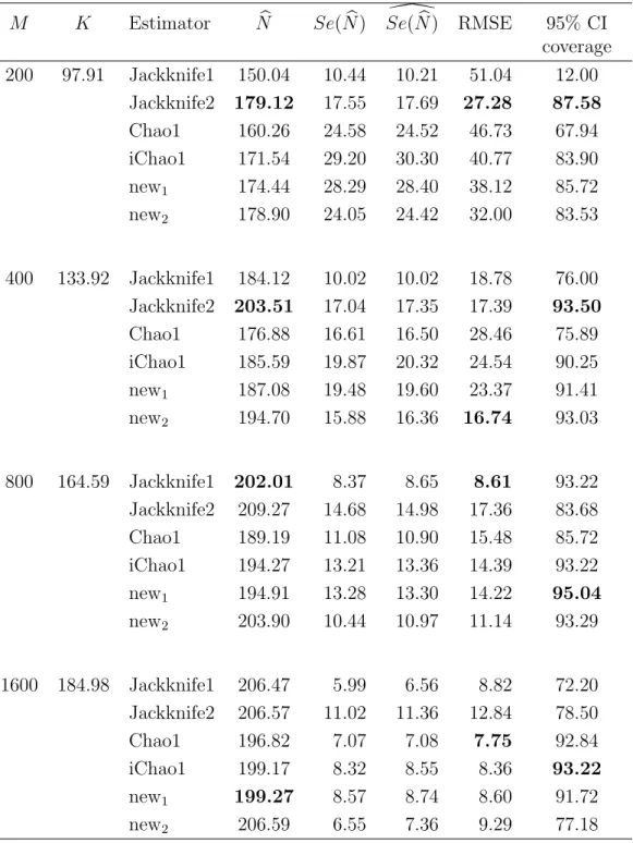
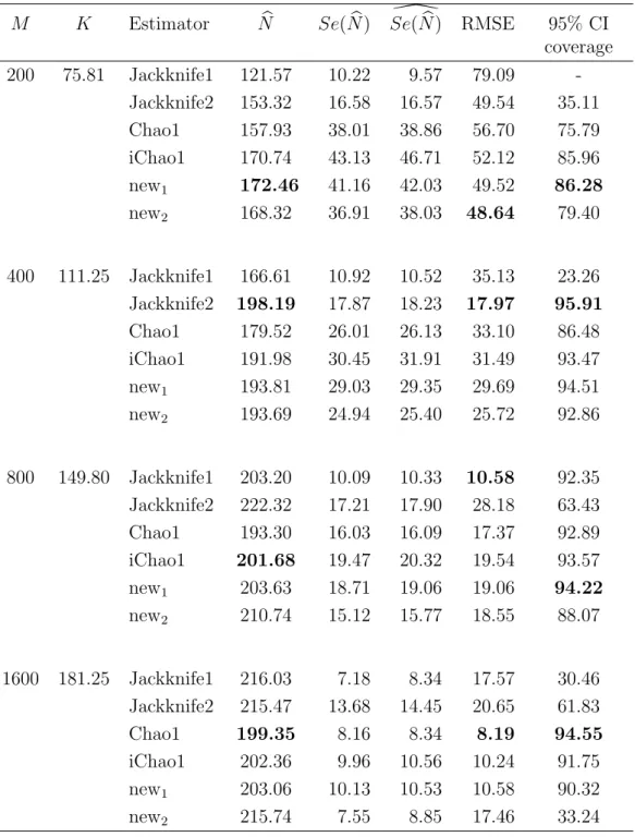
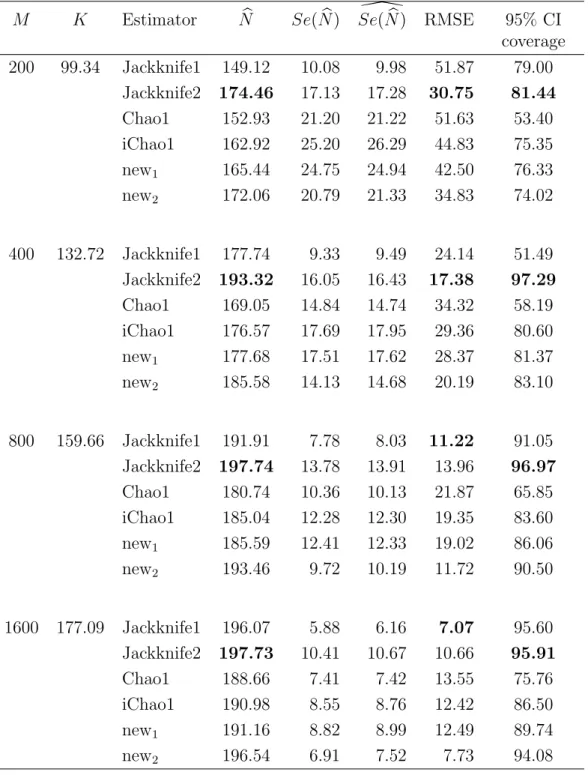
In this Chapter, the literature on species richness estimation is reviewed as follows. In Section 2.2, models of species sample frequency are discussed in-cluding the multinomial and the Poisson models. Species abundance models particularly the heterogeneous models which are used in practice, are discussed in Section 2.3. Nonparametric estimators of species richness are reviewed in Section 2.4. Two novel alternative species richness estimators designed to im-prove upon the Chao1 estimator are introduced in Section 2.5. The mean rel-ative abundance of species seen k times is estimated using various approaches and their performance are investigated in Section 2.6. In Section 2.7, the per-formance of these new estimators is compared with Chao (1984), Chiu et al. (2014) and two jackknife estimators in a simulation study and applied to real data sets in Section 2.8. Finally, conclusions are summarized in Section 2.9.

2.2

Sampling Models

Let N denote the true species richness, the total number of species in the population, andpi (i= 1, . . . , N) be the relative species abundance for species

i or the probability of species i being observed, PN_i₌₁pi = 1. In ecological

applications, this will depend on the difficulty of capturing this species as well as the relative abundance of the species, but we use relative abundance as a convenient shorthand term.

The sample size M denotes the number of individuals collected independently with replacement from the population of N species. Suppose that there are

K distinct species in the sample. Let Xi denote the frequency with which

(31)

the Xi’s have a multinomial distribution which is often calledthe multinomial

model. Alternatively, we may consider the Poisson model that arises when

M is itself a random variable with a Poisson distribution. In this model, the

Xi’s are independent Poisson random variables with Xi ∼P oi(λpi)≡P oi(λi)

and then M _∼ P oi(Pλpi) ≡ P oi(λ). In the multinomial model, the Xi’s

are not independent because they add up to the fixed total M. Note also that in the multinomial model, the marginal distribution of a particular Xi is

Xi ∼Bin(M, pi). Another connection between the two models is that if M is

large and pi is small then the binomial distribution ofXi will be approximated

well by a Poisson distribution with the same mean.

Let fk be the frequency of species seen k times,k = 1,2, . . . , M. We have,

K = kXmax k=1 fk= N X i=1 I(Xi >0),

where kmax is the maximum number of times that any species is seen and

I(Xi >0) = 1 if the event Xi >0 occurs (species i occurs in the sample) and

0 otherwise. The total number of species can be written as

N =E(K) +E(f0), (2.1)

which is a common idea for species richness estimation, where E(K) is the expected number of observed species and E(f0) is the expected number of

unobserved species. E(K) can be estimated by the number of seen species,

K,from the data.

2.3

Species abundance model

Species abundance is a simple method to describe biodiversity. Different ecol-ogy influences the abundance of a species (Huang and Zhan, 2014). The

(32)

com-monness and rarity of species have been described using species abundance models (McGill et al., 2007). The homogeneous model pi = _N1 (i = 1, . . . , N)

is the simplest model to fit the abundance data. However, the chances of collecting different species are typically far from equal in practice. Species abundance data normally exhibit overdispersion, zero inflation and a heavy right tail. These features indicate that a heterogeneous model is required rather than the homogeneous model.

Many models such as negative binomial, log-series, log-normal distributions, broken-stick, Zipf, Zipf-Mandelbrot models and so on have been developed to fit the species abundance data by ecologists (Huang and Zhan, 2014). The pi

can be defined as a function of different abundance model, pi = f(i). When

the Xi’s follow the Poisson distribution, the model of pi’s are discussed into

two groups as follows:

2.3.1

Deterministic models

Deterministic models are used to describe the rank-ordered probabilities (ie.

p1 ≥p2 ≥. . .≥pN) and include the Zipf, Zipf-Mandelbrot, exponential decay

and power decay (a special case of Zipf) models.

The Zipf model

The Zipf model describes the relative abundance rank of the N species. The Zipf model is a discrete probability distribution which is used to model the species abundance distribution and is based on Zipf’s law. It is also known as the power-decay model (Chao et al., 2013). The relative abundance of the ith

ranked species based on the Zipf model is given by

pi =

c

(33)

wherecis the normalising constant, c=PN_i₌₁(1/iα), andα_≥1. Whenα= 0, it gives the homogeneous model, pi = 1/N (Chao and Chiu, 2014).

The Zipf-Mandelbrot model

The Zipf-Mandelbrot model is another model of ranked abundance, which can be defined by

pi =

c

(i+q)α, (i= 1, . . . , N),

where q > ₋1, α _≥ 1 and c is a normalising constant, c = PN_i₌₁(1/(i+q)α₎

(Mouillot and Lepretre, 2000). When q = 0, it reduces to the Zipf model.

Exponential-decay model

The exponential decay model has

pi =c e−βi (i= 1, . . . , N),

where β is the decay rate parameter, β > 0, i is ranked abundance and c is the normalising constant.

2.3.2

Random models

In random models, thepi are drawn as a random sample from some probability

distribution. The resulting pi values are not ordered.

Broken-stick model

A natural distribution to choose is the Dirichlet distribution, since this auto-matically givesPN_i₌₁pi = 1. The general form of the Dirichlet distribution has

parameters θ1, . . . , θN and is generated as

pi = Zi N P i=1 Zi

(34)

where Zi are independent Ga(θi,1) random variables. The broken stick model

has all θi = 1 so that the Zi are independent exp(1) variables.

Therefore, the broken-stick model describes the pattern of species abundance which is given by

pi =cZi (i= 1, . . . , N),

where (Z1, Z2, . . . , ZN) are a random sample from the exponential distribution

with mean 1, and cis the normalising constant (Chao et al., 2013).

Log-normal model

The log-normal model is another distribution used widely for species abun-dance, and is given by

pi =cVi (i= 1, . . . , N),

where (V1, V2, . . . , VN) are a random sample from the log-normal distribution

with parameters, µand σ, and c is the normalising constant. In the study of Chao et al. (2013), species abundances are simulated using this model with parameters µ= 0 andσ = 1.

Negative binomial model

LetU1, U2, . . . , UN are a random sample from the negative binomial

distri-bution with parameter s and r. Then, the species abundance model is given by

pi =cUi (i= 1, . . . , N),

where the probability density function of the negative binomial is

f(U) = (U−1)!

(s₋1)!(U₋s)!(1−r)

(35)

2.3.3

Some numerical examples about species abundance

models

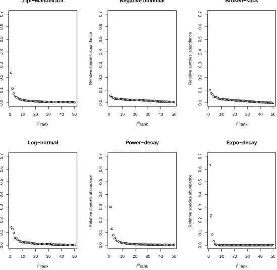
Magurran and Henderson (2011) mention that species abundance data can be presented using a rank abundance plot which is also called a Whittaker plot. The pattern of species abundance is displayed similarly for different models as shown in Figure 2.1. 0 10 20 30 40 50 0.0 0.1 0.2 0.3 0.4 0.5 0.6 0.7 Zipf−Mandelbrot ithrank Relativ e species ab undance 0 10 20 30 40 50 0.0 0.1 0.2 0.3 0.4 0.5 0.6 0.7 Negative binomial ithrank Relativ e species ab undance 0 10 20 30 40 50 0.0 0.1 0.2 0.3 0.4 0.5 0.6 0.7 Broken−stick ithrank Relativ e species ab undance 0 10 20 30 40 50 0.0 0.1 0.2 0.3 0.4 0.5 0.6 0.7 Log−normal ith_rank Relativ e species ab undance 0 10 20 30 40 50 0.0 0.1 0.2 0.3 0.4 0.5 0.6 0.7 Power−decay ith_rank Relativ e species ab undance 0 10 20 30 40 50 0.0 0.1 0.2 0.3 0.4 0.5 0.6 0.7 Expo−decay ith_rank Relativ e species ab undance

Figure 2.1: Probability pi for distinct species i = 1,2, . . . , N, with N =

50 using different models, Zipf-Mandelbrot pi = 1/(i − 0.1), negative

bi-nomial(4,0.04), broken-stick (or Dirichlet(1)), log-normal(0,1), power-decay

pi = 1/i1.2 and expo-decay pi = exp(−i).

The most abundant species is presented at rank 1, the second most abundant species at rank 2 and so on. The exponential-decay model has a long right tail

(36)

with the highest first rank of abundance. The shape of rank abundance plot decreases rapidly compared to other models. For the log-normal, broken-stick and negative-binomial models, relative abundance decreases gradually and pi

is in the range 0 to 0.1. 0 20 40 60 80 100 0.00 0.05 0.10 0.15 0.20 α=0.3 ith_rank pi Zipf Broken−stick Zipf Broken−stick Zipf Broken−stick Zipf Broken−stick Zipf Broken−stick Zipf Broken−stick Zipf Broken−stick Zipf Broken−stick Zipf Broken−stick Zipf Broken−stick Zipf Broken−stick Zipf Broken−stick Zipf Broken−stick Zipf Broken−stick Zipf Broken−stick Zipf Broken−stick Zipf Broken−stick Zipf Broken−stick Zipf Broken−stick Zipf Broken−stick 0 20 40 60 80 100 0.00 0.05 0.10 0.15 0.20 α=0.5 ith_rank pi Zipf Broken−stick Zipf Broken−stick Zipf Broken−stick Zipf Broken−stick Zipf Broken−stick Zipf Broken−stick Zipf Broken−stick Zipf Broken−stick Zipf Broken−stick Zipf Broken−stick Zipf Broken−stick Zipf Broken−stick Zipf Broken−stick Zipf Broken−stick Zipf Broken−stick Zipf Broken−stick Zipf Broken−stick Zipf Broken−stick Zipf Broken−stick Zipf Broken−stick 0 20 40 60 80 100 0.00 0.05 0.10 0.15 0.20 α=0.7 ith_rank pi Zipf Broken−stick Zipf Broken−stick Zipf Broken−stick Zipf Broken−stick Zipf Broken−stick Zipf Broken−stick Zipf Broken−stick Zipf Broken−stick Zipf Broken−stick Zipf Broken−stick Zipf Broken−stick Zipf Broken−stick Zipf Broken−stick Zipf Broken−stick Zipf Broken−stick Zipf Broken−stick Zipf Broken−stick Zipf Broken−stick Zipf Broken−stick Zipf Broken−stick 0 20 40 60 80 100 0.00 0.05 0.10 0.15 0.20 α=0.9 ith_rank pi Zipf Broken−stick Zipf Broken−stick Zipf Broken−stick Zipf Broken−stick Zipf Broken−stick Zipf Broken−stick Zipf Broken−stick Zipf Broken−stick Zipf Broken−stick Zipf Broken−stick Zipf Broken−stick Zipf Broken−stick Zipf Broken−stick Zipf Broken−stick Zipf Broken−stick Zipf Broken−stick Zipf Broken−stick Zipf Broken−stick Zipf Broken−stick Zipf Broken−stick

Figure 2.2: Plot of ranked pi’s values for the Zipf model with N = 100, α in

the range [0.3,0.9] and broken-stick model with 20 simulations.

Relative abundance for Zipf model depends on the parameter α and pi =c/iα

(i = 1, . . . , N). This model explains species abundance data with a similar shape to other models when choosing an appropriate value of α. For example, the Zipf model with α = 0.5 provides the rank species abundance similar to log-normal(0,1) and broken-stick model (Figures 2.2 and 2.3). When α = 0.4, the species abundance curve for the Zipf model displays the same results as negative binomial model NB(4,0.04) (Figure 2.4). Whenα = 2, the Zipf model gives the species abundance which are similar the expo-decay model (Figure 2.5).

(37)

0 20 40 60 80 100 0.00 0.05 0.10 0.15 0.20 α=0.3 ith_rank pi Zipf Log−normal Zipf Log−normal Zipf Log−normal Zipf Log−normal Zipf Log−normal Zipf Log−normal Zipf Log−normal Zipf Log−normal Zipf Log−normal Zipf Log−normal Zipf Log−normal Zipf Log−normal Zipf Log−normal Zipf Log−normal Zipf Log−normal Zipf Log−normal Zipf Log−normal Zipf Log−normal Zipf Log−normal Zipf Log−normal 0 20 40 60 80 100 0.00 0.05 0.10 0.15 0.20 α=0.5 ith_rank pi Zipf Log−normal Zipf Log−normal Zipf Log−normal Zipf Log−normal Zipf Log−normal Zipf Log−normal Zipf Log−normal Zipf Log−normal Zipf Log−normal Zipf Log−normal Zipf Log−normal Zipf Log−normal Zipf Log−normal Zipf Log−normal Zipf Log−normal Zipf Log−normal Zipf Log−normal Zipf Log−normal Zipf Log−normal Zipf Log−normal 0 20 40 60 80 100 0.00 0.05 0.10 0.15 0.20 α=0.7 ith_rank pi Zipf Log−normal Zipf Log−normal Zipf Log−normal Zipf Log−normal Zipf Log−normal Zipf Log−normal Zipf Log−normal Zipf Log−normal Zipf Log−normal Zipf Log−normal Zipf Log−normal Zipf Log−normal Zipf Log−normal Zipf Log−normal Zipf Log−normal Zipf Log−normal Zipf Log−normal Zipf Log−normal Zipf Log−normal Zipf Log−normal 0 20 40 60 80 100 0.00 0.05 0.10 0.15 0.20 α=0.9 ith_rank pi Zipf Log−normal Zipf Log−normal Zipf Log−normal Zipf Log−normal Zipf Log−normal Zipf Log−normal Zipf Log−normal Zipf Log−normal Zipf Log−normal Zipf Log−normal Zipf Log−normal Zipf Log−normal Zipf Log−normal Zipf Log−normal Zipf Log−normal Zipf Log−normal Zipf Log−normal Zipf Log−normal Zipf Log−normal Zipf Log−normal

the range [0.3,0.9] and log-normal(0,1) model 20 simulations.

0 20 40 60 80 100 0.00 0.05 0.10 0.15 α=0.2 ith_rank pi Zipf NB Zipf NB Zipf NB Zipf NB Zipf NB Zipf NB Zipf NB Zipf NB Zipf NB Zipf NB Zipf NB Zipf NB Zipf NB Zipf NB Zipf NB Zipf NB Zipf NB Zipf NB Zipf NB Zipf NB 0 20 40 60 80 100 0.00 0.05 0.10 0.15 α=0.4 ith_rank pi Zipf NB Zipf NB Zipf NB Zipf NB Zipf NB Zipf NB Zipf NB Zipf NB Zipf NB Zipf NB Zipf NB Zipf NB Zipf NB Zipf NB Zipf NB Zipf NB Zipf NB Zipf NB Zipf NB Zipf NB 0 20 40 60 80 100 0.00 0.05 0.10 0.15 α=0.6 ith_rank pi Zipf NB Zipf NB Zipf NB Zipf NB Zipf NB Zipf NB Zipf NB Zipf NB Zipf NB Zipf NB Zipf NB Zipf NB Zipf NB Zipf NB Zipf NB Zipf NB Zipf NB Zipf NB Zipf NB Zipf NB 0 20 40 60 80 100 0.00 0.05 0.10 0.15 α=0.8 ith_rank pi Zipf NB Zipf NB Zipf NB Zipf NB Zipf NB Zipf NB Zipf NB Zipf NB Zipf NB Zipf NB Zipf NB Zipf NB Zipf NB Zipf NB Zipf NB Zipf NB Zipf NB Zipf NB Zipf NB Zipf NB

(38)

0 20 40 60 80 100 0.0 0.2 0.4 0.6 0.8 1.0 α=1 ith_rank pi Zipf Expo−decay Zipf Expo−decay Zipf Expo−decay Zipf Expo−decay Zipf Expo−decay Zipf Expo−decay Zipf Expo−decay Zipf Expo−decay Zipf Expo−decay Zipf Expo−decay Zipf Expo−decay Zipf Expo−decay Zipf Expo−decay Zipf Expo−decay Zipf Expo−decay Zipf Expo−decay Zipf Expo−decay Zipf Expo−decay Zipf Expo−decay Zipf Expo−decay 0 20 40 60 80 100 0.0 0.2 0.4 0.6 0.8 1.0 α=2 ith_rank pi Zipf Expo−decay Zipf Expo−decay Zipf Expo−decay Zipf Expo−decay Zipf Expo−decay Zipf Expo−decay Zipf Expo−decay Zipf Expo−decay Zipf Expo−decay Zipf Expo−decay Zipf Expo−decay Zipf Expo−decay Zipf Expo−decay Zipf Expo−decay Zipf Expo−decay Zipf Expo−decay Zipf Expo−decay Zipf Expo−decay Zipf Expo−decay Zipf Expo−decay 0 20 40 60 80 100 0.0 0.2 0.4 0.6 0.8 1.0 α=3 ith_rank pi Zipf Expo−decay Zipf Expo−decay Zipf Expo−decay Zipf Expo−decay Zipf Expo−decay Zipf Expo−decay Zipf Expo−decay Zipf Expo−decay Zipf Expo−decay Zipf Expo−decay Zipf Expo−decay Zipf Expo−decay Zipf Expo−decay Zipf Expo−decay Zipf Expo−decay Zipf Expo−decay Zipf Expo−decay Zipf Expo−decay Zipf Expo−decay Zipf Expo−decay 0 20 40 60 80 100 0.0 0.2 0.4 0.6 0.8 1.0 α=4 ith_rank pi Zipf Expo−decay Zipf Expo−decay Zipf Expo−decay Zipf Expo−decay Zipf Expo−decay Zipf Expo−decay Zipf Expo−decay Zipf Expo−decay Zipf Expo−decay Zipf Expo−decay Zipf Expo−decay Zipf Expo−decay Zipf Expo−decay Zipf Expo−decay Zipf Expo−decay Zipf Expo−decay Zipf Expo−decay Zipf Expo−decay Zipf Expo−decay Zipf Expo−decay

Figure 2.5: Plot of rankedpi’s values for the Zipf model and expo-decay model

with N = 100, α in the range [1,4].

2.4

Nonparametric approach

Nonparametric estimators are useful methods as there are no requirements about assumptions for community structure (Chiarucci et al., 2003). Many estimators have been proposed for estimating the number of species and these are constructed based on the number of seen and unseen species. In particu-lar, the number of unseen species is key for species richness estimation. The following nonparametric estimators are reviewed in this section.

2.4.1

Good-Turing estimator

Good-Turing estimation is a simple technique that estimates the number of un-seen species using the frequency of singletons (species observed exactly once) in the sample, f1 =PNi=1I(Xi = 1). Because Good (1953) credits this idea to

(39)

The following explanation of the Good-Turing estimator is based on Chiu et al. (2014). Recall thatM is the sample size or the number of individuals observed,

M =Pkmax

k=1 kfk, wherefk is the frequency of species seenk times. The mean

relative abundance of the species seen k times in the sample, denoted asαk, is

αk=

PN

i=1piI(Xi =k)

fk

, k = 0,1, . . . .

Good (1953) proposed that αk could be estimated by

b αk= (k+ 1) M fk+1 fk . (2.2)

By definition of αk, the total relative abundance of all species seen k times is

αkfk which can be estimated by

b αkfk= (k+ 1)fk+1 M . In particular, for k = 0, b α0f0 = f1 M

is the estimated total relative abundance of all unseen species,PN_i₌₁piI(Xi = 0).

Then, the expected number of unobserved species is

E(f0) =M N

X

i=1

piI(Xi = 0) =M α0f0 =f1.

Hence, the Good-Turing estimator of the number of species based on equation (2.1) is

b

NG=K+f1. (2.3)

This form of the Good-Turing estimator is given for example by Hidaka (2014) as his estimator NbGT. This is also approximately the first-order jackknife

estimator in Section 2.4.4, if the factor (M −1)

(40)

(2014).

2.4.2

Chao1 Estimator

Chao (1984) proposed an estimator of a lower bound for species richness, al-though in practice it is often used as an estimator of species richness itself. Rare species have been considered in order to construct this estimator, which is based only on the number of species seen once and twice. Recall that Xi

is the species frequency for species i in the sample and pi is the probability

that a randomly selected individual belongs to species i. The estimator can be derived under the multinomial and the Poisson sampling models as follows:

Multinomial Model

Under the multinomial sampling model, Xi ∼Bin(M, pi) which implies that

E(fk) = E _N P i=1 I(Xi = 0) = N P i=1 M k pk i(1−pi)M−k, k = 0,1,2, . . . , M. (2.4)

The Cauchy-Schwarz inequality states that for any ai, bi ∈R, N X i=1 a2_i N X i=1 b2_i_≥ N X i=1 aibi !2 . (2.5)

Setting ai = (1−pi)M/2, bi =pi(1−pi)M/2−1 and aibi =pi(1−pi)M−1, gives

_N P i=1 (1₋pi)M N P i=1 p2 i(1−pi)M−2 ≥ _N P i=1 pi(1−pi)M−1 2 , E(f0) 1 M 2 E(f2) ≥ 1 M2[E(f1)] 2 , E(f0) ≥ (M₋1) M [E(f1)]2 2E(f2) .

(41)

Using equation (2.1), a lower bound for the number of species becomes N >E(K) + (M−1) M [E(f1)]2 2E(f2) ,

which can be estimated using the observed data as

b NChao1 =K+ (M ₋1) M f2 1 2f2 , (2.6)

where f1 and f2 are the number of species seen once and twice.

The standard asymptotic approach known as the delta method is used for estimating the variance of NbChao1 (Chiu et al., 2014).

c var(NbChao1) = n X i=1 n X j=1 ∂NbChao1 ∂fi ∂NbChao1 ∂fj c cov(fi, fj), where c cov(fi, fj) =        fi(1−fi/NbChao1), if i=j; −fifj/NbChao1, if i6=j.

After some algebra, the variance estimator is derived as

c var(NbChao1) =f2 " 1 4 M−1 M 2 f1 f2 4 + M−1 M 2 f1 f2 3 +1 2 M−1 M f1 f2 2# (2.7) Poisson Model

When M is large and p is small, the expected number of species seen k times can be approximated using the Poisson distribution withλi =N pi which gives

E(fk) = N P i=1 λk i e−λi k! , k = 0,1,2, . . . , M. (2.8)

(42)

aibi =λie−λi, the lower bound for E(f0) is given by hPN i=1e−λi i hPN i=1λ2ie−λi i ≥ hPNi=1λie−λi i2 , E(f0) 2E(f2) ≥ [E(f1)]2, E(f0) ≥ [E(f1)]2 2E(f2) ,

which again leads to the estimator

b NChao1 =K+ f2 1 2f2 . (2.9)

When M is large, the variance estimator of NbChao1 in equation (2.7) can be

reduced as (Chao, 1987) Var(NbChao1) = f2 " 1 4 f1 f2 4 + f1 f2 3 +1 2 f1 f2 2# . (2.10)

When the estimator breaks down atf2 = 0, a modified bias-corrected estimator

is proposed b NChao1 =K + f1(f1−1) 2(f2+ 1) . (2.11)

The Chao1 estimator is extended in the study of Chiu et al. (2014) using the first four frequencies of distinct species and by Lanumteang and B¨ohning (2011) using the first three frequencies of distinct species. In the next section, the improved Chao1 estimator by Chiu et al. (2014) is investigated and compared to the original Chao1 estimator.

2.4.3

iChao1 estimator

An improved Chao1 estimator called iChao1 is developed by Chiu et al. (2014) based on a modified Good-Turing frequency formula. The new estimator ob-tains a new lower bound using the number of singletons, doubletons, tripletons and quadrupletons (i.e. f1, f2, f3 and f4). The improved estimator by Chiu

(43)

bias, in particular when relative abundances are highly heterogeneous.

Chiu et al. (2014) proposed estimating the true mean relative abundance of species seen k times as

b

αk=

(k+ 1)fk+1

(M ₋k)fk+ (k+ 1)fk+1

, k = 1,2, . . . , (2.12)

The new lower bound is derived by considering the magnitude of the first-order bias of NbChao1 which can be derived as

|bias(NbChao1)| = E(f0)− (M ₋1) M E(f1)2 2E(f2) = E(f0){2E(f2)/[M(M −1)]} −[E(f1)/M] 2 2E(f2)/[M(M −1)] ≈ " 1₋α3 α3 1₋α1 α1 − 1₋α3 α3 2# × _N P i=1 pi(1−pi)n−1 × _N P i=1 p3 i(1−pi)n−3 ,

and applying the Cauchy Schwarz inequality yields

" _N X i=1 pi(1−pi)n−1 # × " _N X i=1 p3_i(1₋pi)n−3 # ≥ " _N X i=1 p2_i(1₋pi)n−2 #2 .

Hence, the approximate bias of the estimator becomes

|bias(NbChao1)| ≈ " 1₋α3 α3 1₋α1 α1 − 1₋α3 α3 2# × _N P i=1 p2 i(1−pi)n−2 2 ≈ 1−_αα3 3 1₋α1 α1 − 1₋α3 α3 2E(f2) M(M ₋1). (2.13) Using the modified Good-Turing frequency in equation (2.12), we obtain the

(44)

improved Chao1 estimator as NbChao1+|bias(NbChao1)|, that is, b NiChao1 =NbChao1+ (M ₋3) 4M f3 f4 × max f1− (M ₋3) 2(M ₋1) f2f3 f4 ,0 . (2.14)

When f4 = 0, it is replaced by f4 + 1. For large sample size or equal species

abundance, the iChao1 estimator is close to being an asymptotically unbiased estimator which leads to good approximation (Chiu et al., 2014). On the other hand, a negative bias may exist for unequal species abundance or small sample size (Chao and Chiu, 2014).

When M is large, equation (2.14) can be simplified to

b NiChao1 =NbChao1+ f3 4f4 × max f1− f2f3 2f4 ,0 . (2.15)

The variance of iChao1 estimator can be approximated using the delta method by c var(NbiChao1)≈ ▽g       f0 f1 f2 f3 f4       T c cov       f0 f1 f2 f3 f4      ▽g       f0 f1 f2 f3 f4      , (2.16) where ▽g       f0 f1 f2 f3 f4      = ∂Nb ∂f0 ∂Nb ∂f1 ∂Nb ∂f2 ∂Nb ∂f3 ∂Nb ∂f4 T ,

with Nb =NbiChao1. The partial derivatives

∂Nb ∂fi for j = 0,1,2,3,4 are ∂Nb ∂f0 =₋1, ∂Nb ∂f1 = 1 4 4f1f4(M−1) +f2f3(M −3) M f2f4 ,

(45)

∂Nb ∂f2 =₋1 8 4f2 1f42(M −1)2+f22f32(M −3)2 M(M ₋1)f2 2f42 , ∂Nb ∂f3 = (M −3) 4 (f1f4(M −1)−f2f3(M −3)) M(M ₋1)f2 4 , ∂Nb ∂f4 =₋(M −3)f3 4 (f1f4(M −1)−f2f3(M −3)) M(M ₋1)f3 4 .

and the variance-covariance matrix of the multinomial vector (f0, f1, f2, f3, f4)T

can be estimated by c cov       f0 f1 f2 f3 f4      =                 f0 1₋ f0 N −f_N0f1 −f0_Nf2 −f_N0f3 −f_N0f4 −f_N0f1 f1 1₋ f1 N −f1_Nf2 −f_N1f3 −f_N1f4 −f_N0f2 −f_N1f2 f2 1₋f2 N −f_N2f3 −f_N2f4 −f0f3 N − f1f3 N − f2f3 N f3 1₋ f3 N −f3f4 N −f0f4 N − f1f4 N − f2f4 N − f3f4 N f4 1₋ f4 N                 .

For practical calculation,f0andN can be replaced byfˆ0=

(M₋1)f2 1

2M f2

+_|bias(NbChao1)|

and NbiChao1. For the homogeneous model, the expected value of f1−f2f3/2f4

tends to zero as the sample size increases. Then, the iChao1 estimator can be replaced by the Chao1 estimator (Chiu et al., 2014) .

2.4.4

Jackknife estimators

Jackknife estimators were proposed by Quenouille (1949) and expanded by Tukey (1958). Suppose we have a biased estimator, θb, of a parameter θ. The basic idea of the jackknife method is to calculate a series of estimators bθ−i,

missing out the ith _{sample observation and calculate the new estimators}

b θ_J(1) =Mθb₋ M₋1 M _XM i=1 b θ−i.

(46)

bias compared to θb.

Jackknife estimators of species richness were introduced by Burnham and Over-ton (1978). The basic estimator isθb=K, the observed number of species. Let

b

θ−i be the number of distinct species by leaving out species i, which is given

by b θ−i =       

K ₋1 if speciesXi seen only once,

K otherwise.

.

The first-order jackknife estimator can therefore be derived as

b N_J(1) =Mθb₋ M ₋1 M _XM i=1 b θ−i =M K₋ M ₋1 M {f1(K −1) + (M−f1)K} =M K₋ M ₋1 M {M K₋f1} =M K₋(M ₋1)K+ M ₋1 M f1 =K + M ₋1 M f1. (2.17)

It is also possible to derive higher-order jackknife estimators by omitting more than one observation from the sample. The second-order jackknife estimator involves estimators bθ−ij, calculated by excluding each pair of observations i, j

from the sample. The general formula for the second-order jackknife estimator is b θ_J(2) = 1 2 ( M2θb₋ 2(M −1) 2 M M X i=1 b θ−i+ 2(M ₋2)2 M(M₋1) X i<j b θ−ij ) .

(47)

by leaving out samples i and j b θ−ij =               

K ₋2 if speciesXi and Xj both seen once,

K ₋1 if either speciesXi or species Xj seen once,

K otherwise.

Burnham and Overton (1978) show that this leads to the estimator

b N_J(2) = 1 2 ( M2θb₋ 2(M −1) 2 M M X i=1 b θ−i+ 2(M ₋2)2 M(M ₋1) X i<j b θ−ij ) =K+ (2M −3)f1 M − (M ₋2)2_f 2 M(M₋1). (2.18)

In practice, simplified forms of these estimators are often used, based on large values of M

b

N_J(1) =K+f1 (2.19)

b

N_J(2) =K+ 2f1−f2. (2.20)

The result in equation (2.22) shows that the first-order Jackknife estimator is identical to the Good-Turing estimator in equation (2.3) when M is large.

Burnham and Overton (1978) proposed the general simplified formula for the

kth_{-order jackknife estimator which is given by}

b N_J(k)=K+ k X j=1 (₋1)j+1 k j fj. (2.21)

Ji-Ping Wang developed the R package called SPECIES in 2011 which pro-vides a function jackknife to calculate these estimators.

(48)

species which are seen only once. For the second order jackknife estimator, it is formed using both the number of species seen once and the number seen twice. The bias and variance of estimator are balanced by choosing the k th-order. A higher order is appropriate for improving bias. However, this might lead to a higher variance of estimator (Wang, 2011).

Under the distribution of K and the expectation of f1 in equation (2.4), the

expected value of the first-order jackknife estimator can be derived as

E(Nb_J(1)) = E(K) + M−1 M E(f1) = E(K) + M−1 M N P i=1 M 1 pi(1−pi)M−1 = E(K) + (M₋1) N P i=1 pi(1−pi)M−1. where E(K) = N₋PN i=1

(1₋pi)M (Hidaka, 2014). Then, we have

Bias(Nb_J(1)) = E(Nb_J(1))₋N = N X i=1 (1₋pi)M + (M −1) N X i=1 pi(1−pi)M−1. (2.22)

(49)

estima-tor can be written as E(Nb_J(2)) = E(K) + (2M −3) M E(f1)− (M ₋2)2 M(M ₋1) E(f2) = N ₋ N P i=1 (1₋pi)M + (2M ₋3) M N P i=1 M 1 pi(1−pi)M−1 − (M₋2)2 M(M₋1) N P i=1 M 2 pi(1−pi)M−2 = N ₋ N P i=1 (1₋pi)M + (2M −3) N P i=1 pi(1−pi)M−1 − (M ₋2)2 2 N P i=1 p2i(1−pi)M−2,

and this gives

Bias(Nb_J(2)) = E(Nb_J(2))₋N = N X i=1 (1₋pi)M + (2M −3) N X i=1 pi(1−pi)M−1 − (M ₋2)2 2 N X i=1 p2_i(1₋pi)M−2. (2.23)

2.4.5

Horvitz-Thompson estimator

The Horvitz-Thompson (HT) estimator is an unbiased estimator of the popu-lation sizeN proposed by Horvitz and Thompson (1952). It is applied in many fields including the problem of estimating the number of species in ecology and estimating vocabulary size in linguistics, for example B¨ohning (2008), Cruyff and van der Heijden (2008) and Hidaka (2014). Assume πi is the probability

that species i is included in the sample, termed the inclusion probability. The estimator of species richness is given by

b NH = M X i=1 fi πi . (2.24)

(50)

An unbiased estimator of variance is d Var(NbH) = M X i=1 1₋πi π2 i y_i2+ M X i=1 X i6=j πij −πiπj πiπjπij yiyj, (2.25)

where πi = 1−(1−pi)M is the inclusion probability of species i and πij =

πi+πj −

1₋(1₋pi−pj)M

is the inclusion probability for species i and j.

The species abundance model or the probability of species i collected is un-known in practice. The Horvitz-Thompson-Like estimator is an alternative estimator which can be used instead of the Horvitz-Thompson estimator. The unknown probabilitypiis replaced byi/M. Then, the Horvitz-Thompson-Like

estimator is given by (McCrea and Morgan, 2014)

b NHL = M X i=1 fi 1₋ 1₋ i M M. (2.26)

2.5

An alternative improvement to the Chao1

estimator

In this section, two new estimators of species richness are developed using α_bk

based on the Good-Turing coverage estimator. The sample coverage is the pro-portion of all individuals in the population belonging to the observed species in the sample. The concept of the sample coverage is presented in an example of Chao and Jost (2012) who discussed the sample coverage of a terrestrial arthropod community with 50 species. Assume that the relative abundance of species 1 is 0.3, species 2 is 0.1, species 3 through 5 is 0.05 each and species 6 through 50 are 0.01 each. In sample of 20 individuals, there are 12 species collected (e.g. species 1, 2, 3, 4, 5, 6, 9, 14, 23, 27, 41, 47) and then the sample coverage is 62% (0.3 + 0.1 + 0.05_×3 + 0.01_×7). This means there is 62% of

(51)

all individuals belonging to the observed species in the sample.

Good (1953) proposed estimating the sample coverage using

b C = N X i=1 piI(Xi = 0) = 1−α0f0 = 1− f1 M.

Then, an estimator for the true mean relative abundance of species seen k

times based on the Good-Turing coverage approach is given by

b αk = 1₋ f1 M k M. (2.27)

The following two new estimators, Nbnew1 and Nbnew2, are constructed using

the same idea of the iChao1 estimator. The bias of NbChao1 is estimated using

equation (2.13). The Nbnew1 estimator is constructed using αb1 by Chiu et al.

(2014) in equation (2.12) and α_b3 by equation (2.27). This provides

b Nnew1=NbC+ 1 9 (3M f1(M−1)−2M f2(M−3)−3f12(M−1)−6f1f2) (M2−3(M−f1)) M(M−1)(M−f2)2 . (2.28) The Nbnew2 estimator estimates both αb1 and αb3 by equation (2.27), giving

b Nnew2 =NbC + 4 9 (M2₋₃_M _{+ 3}_f 1)M f2 (M ₋1)(M₋f1)2 . (2.29) The delta method is used to estimate the variance of both alternative estima-tors followings the same approach as for the iChao1 estimator. The formulae are lengthy and are not given here, but are incorporated into R code.

(52)

2.6