THE CENTRAL CURVE IN LINEAR PROGRAMMING
JES ´US A. DE LOERA, BERND STURMFELS, AND CYNTHIA VINZANT
Abstract. The central curve of a linear program is an algebraic curve specified by linear and quadratic constraints arising from complementary slackness. It is the union of the various central paths for minimizing or maximizing the cost function over any region in the associated hyperplane arrangement. We determine the degree, arithmetic genus and defining prime ideal of the central curve, thereby answering a question of Bayer and Lagarias. These invariants, along with the degree of the Gauss image of the curve, are expressed in terms of the matroid of the input matrix. Extending work of Dedieu, Malajovich and Shub, this yields an instance-specific bound on the total curvature of the central path, a quantity relevant for interior point methods. The global geometry of central curves is studied in detail.
1. Introduction
We consider the standard linear programming problem in itsprimalanddualformulation: (1) Maximize cTx subject to Ax=b and x≥0;
(2) Minimize bTy subject to ATy−s=c and s≥0.
Here A is a fixed matrix of rank d having n columns, while the vectors c ∈ Rn and b ∈
image(A) may vary. Before describing our contributions, we review some basics from the theory of linear programming [22, 29]. The logarithmic barrier function for (1) is defined as
fλ(x) := cTx + λ n
X
i=1
logxi,
where λ >0 is a real parameter. This specifies a family of optimization problems: (3) Maximize fλ(x) subject to Ax=b and x≥0.
Since the function fλ is strictly concave, it attains a unique maximum x∗(λ) in the interior
of the feasible polytope P = {x ∈ Rn
≥0 : Ax = b}. Note that fλ(x) tends to −∞ when x
approaches the boundary of P. The primal central path is the curve {x∗(λ)|λ > 0} inside the polytopeP. There is an analogous logarithmic barrier function for the dual problem (2) and a correspondingdual central path. The central path connects the optimal solution of the linear program in question with its analytic center. It is homeomorphic to a line segment.
The complementary slackness condition says that the pair of optimal solutions, to the primal linear program (1) and to the dual linear program (2), are characterized by
(4) Ax=b, ATy−s=c, x≥0, s≥0, and xisi = 0 for i= 1,2, . . . , n.
The central path converges to the solution of this system of equations and inequalities:
2010Mathematics Subject Classification. Primary: 90C05; Secondary: 05B35, 13P25, 14H45, 52C35.
Key words and phrases. Linear programming, interior point methods, matroid, Tutte polynomial, hyper-bolic polynomial, Gauss map, degree, curvature, projective variety, Gr¨obner basis, hyperplane arrangement.
Figure 1. The central curve of a hexagon for two choices of the cost function
Theorem 1 (cf. [29]). For all λ >0, the system of polynomial equations
(5) Ax=b, ATy−s=c, and xisi =λ for i= 1,2, . . . , n,
has a unique real solution (x∗(λ),y∗(λ),s∗(λ)) with the properties x∗(λ)>0 and s∗(λ)>0. The point x∗(λ) is the optimal solution of (3). The limit point (x∗(0),y∗(0),s∗(0)) of these solutions for λ→0 is the unique solution of the complementary slackness constraints (4).
Our object of study in this paper is the set of all solutions of the equations (5), not just those whose coordinates are real and positive. For general b and c, this set is the following irreducible algebraic curve. Thecentral curve is the Zariski closure of the central path, that is, the smallest algebraic variety in (x,y,s)-space, R2n+d, that contains the central path.
The primal central curve inRn is obtained by projecting the central curve intox-space. We
can similarly define the dual central curve by projecting intoy-space or into s-space.
Example 2. Figure 1 depicts the primal central curve for a small transportation problem. HereA is the 5×6 node-edge matrix of the complete bipartite graph K2,3, as shown below:
v1 v2 v3 v4 v5 v1 1 1 1 0 0 0 v2 0 0 0 1 1 1 v3 1 0 0 1 0 0 v4 0 1 0 0 1 0 v5 0 0 1 0 0 1
Heren = 6 andd= 4 because A has rank 4. We return to this example in Section 4. As seen in Figure 1, the primal central curve contains the central paths of every polytope in the arrangement in{Ax=b}defined by the coordinate hyperplanes {xi = 0}. The union
over all central curves, as the right hand side b varies, is an algebraic variety of dimension d+ 1, called the central sheet, which will play an important role. Our analysis will rely on
recent advances on the understanding of algebras generated by reciprocals of linear forms as presented in [5, 20, 27]. Matroid theory will be our language for working with these objects. The algebro-geometric study of central paths was pioneered by Bayer and Lagarias [2, 3]. Their 1989 articles are part of the early history of interior point methods. They observed (on pages 569-571 of [3]) that the central path defines an irreducible algebraic curve in x-space ory-space, and they identified a complete intersection that has the central curve as an irreducible component. The last sentence of [3, §11] states the open problem of identifying polynomials that cut out the central curve, without any extraneous components. It is worth stressing that while one can easily find equations for the central curve from the first derivative optimality conditions on the barrier function, those yield, in general, extra spurious solutions. In Section 4 of this article we present a complete solution to the Bayer-Lagarias problem. Under the assumption that b and c are general, while A is fixed and possibly special, we determine the prime ideal of all polynomials that vanish on the primal central curve. We express the degree of this curve as a matroid invariant read from the linear program. This yields a tight upper bound n−d1
for the degree. For instance, the curves in Figure 1 have degree 5. We also determine the Hilbert series and arithmetic genus of its closure in Pn−1.
In Section 6, we give an entirely symmetric description of the primal-dual central curve inside a product of two projective spaces. This leads to a range of results on the global geometry of our curves. In particular, we explain precisely how the central curve passes through all vertices of the hyperplane arrangement and through all the analytic centers.
In practical computations, the optimal solution to (1) is found by following a piecewise-linear approximation to the central path. Different strategies for generating the step-by-step moves correspond to different interior point methods. One way to estimate the number of Newton steps needed to reach the optimal solution is to bound the total curvature of the central path. This has been investigated by many authors (see e.g. [8,18,24,30,32]), the idea being that curves with small curvature are easier to approximate with line segments.
Section 5 develops our approach to estimating the total curvature of the central curve. Dedieu, Malajovich and Shub [8] noted that the total curvature of any curveC coincides with the arc length of the image of C under the Gauss map. Hence any bound on the degree of theGauss curvetranslates into a bound on the total curvature. Our main result in Section 5 is a very precise bound for the degree of the Gauss curve arising from any linear program.
Our formulas and bounds in Sections 4, 5, and 6 are expressed in the language of matroid theory. A particularly important role is played by matroid invariants, such as the Tutte polynomial, that are associated with the matrix A. Section 3 is devoted to an introductory exposition of the required background from matroid theory and geometric combinatorics.
Section 2 offers an analysis of central curves in the plane, with emphasis on the dual formulation (d= 2). We shall see that planar central curves areVinnikov curves[31] of degree n−1 that are derived from an arrangement of n lines by taking a Renegar derivative [21]. The total curvature of a plane curve can be bounded in terms of its number of real inflection points, and we shall derive a new bound from a classical formula due to Felix Klein [15].
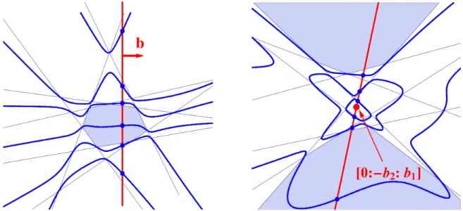
What got us started on this project was our desire to understand the “snakes” of Deza, Terlaky and Zinchenko [10]. We close the introduction by presenting their curve for n= 6. Example 3. Letn= 6, d= 2 and fix the following matrix, right hand side and cost vector:
A= 0 −1 1 −1 1 −1 −1 101 13 10011 100011 1000011 , b = 0 1 ,
Figure 2. The DTZ snake with 6 constraints. On the left, a global view of
the polygon and its central curve with the liney2 = 1 appearing as part of the curve. On the right a close-up of the central path and its inflection points.
cT = −1 −1 2 − 1 3 − 449989 990000 − 359989 792000 − 299989 660000 .
The resulting linear program, in its dual formulation (2), is precisely the instance in [10, Fig-ure 2, page 218]. We redrew the central curve in FigFig-ure 2. The hexagon P6∗,2 shown there equals {y∈R2 : yA≥cT}. The analytic center ofP∗
6,2 is a point with approximate coordi-nates y= (−0.027978...,0.778637...). It has algebraic degree 10 overQ, which indicates the level of difficulty to write exact coordinates. The optimal solution is the vertex with rational coordinates y= (y1, y2) = (−1800660000599700011,−600220000519989 ) = (−0.033304...,−0.00086...).
Following [10], we sampled many points along the central path, and we found that the total curvature of the central path equals 13.375481417.... This measurement concerns only the part of the central curve that goes from the analytic center to the optimum. Our algebraic recipe (7) for computing the central curve leads to the following polynomial: (y2−1) 2760518880000000000000000y4 2+ 22783991895360000000000000y23y1−1559398946696532000000000y32+ 1688399343321073200000000y1y2 2+87717009913470910818000y22−3511691013758400000000000y21y22−324621326759441931317y2 + 11183216292449806548000y1y2+ 2558474824415400000000y2 1y2−51358431801600000000000y31y2+ 6337035495096700140y1 + 77623920000000000000y4 1−13856351760343620000y21+ 291589604847546655−38575873512000000000y13 .
This polynomial of degree 5 has a linear factor y2 −1 because the vector b that specifies the objective function in this dual formulation is parallel to the first column of A. Thus the curve in Figure 2 has degree 4, and its defining irreducible polynomial is the second factor. When the cost vectorb is replaced by a vector that is not parallel to a column ofAthen the output of the same calculation (to be explained in Section 4) is an irreducible polynomial of degree 5. In other words, for almost all choices of b, the central curve is a quintic curve.
While most studies in optimization focus only on just the small portion of the curve that runs from the analytic center to the optimum, we argue here that the algebraic geometry of the entire curve reveals a more complete and interesting picture. The entire central curve is a quintic that passes through all vertices of the line arrangement defined by the six edges of the polygon. As we shall see, the central curve passes through the analytic centers of all bounded cells (Theorem 28) and it is topologically a nested set of ovals (Proposition 4).
2. Plane Curves
When the central curve lives in a plane, the curve is cut out by a single polynomial equation. This occurs for the dual curve when d= 2 and the primal curve when n=d−2. We now focus on the dual curve (d = 2). This serves as a warm-up to the full derivation of all equations in Section 4. In this section we derive the equations of the central curve from first principles, we show that these curves are hyperbolic and Renegar derivatives of a product of lines, and we use this structure to bound the average total curvature of the curve. Let A = (aij) be a fixed 2×n matrix of rank 2, and consider arbitrary vectors b =
(b1, b2)T ∈R2 andc= (c1, . . . , c
n)T ∈Rn. Here they-space is the planeR2 with coordinates (y1, y2). The central curve is the Zariski closure in this plane of the parametrized path
y∗(λ) = argmin y∈R2 b1y1+b2y2−λ n X i=1 log(a1iy1+a2iy2+ci).
The conditions for optimality are obtained by setting the first partial derivatives to zero:
0 = b1 −λ n X i=1 a1i a1iy1+a2iy2 +ci and 0 = b2−λ n X i=1 a2i a1iy1 +a2iy2+ci . Multiplying these equations by b2/λ orb1/λ gives
(6) b1b2 λ = n X i=1 b2a1i a1iy1+a2iy2+ci = n X i=1 b1a2i a1iy1+a2iy2+ci .
This eliminates the parameterλ and we are left with the equation on the right. By clearing denominators, we get a single polynomial C that vanishes on the central curve in y-space: (7) C(y1, y2) = X i∈I (b1a2i−b2a1i) Y j∈I\{i} (a1jy1+a2jy2 +cj),
whereI ={i : b1a2i−b2a1i 6= 0}. We see that the degree ofC(y) is|I|−1. This equalsn−1
for generic b. In our derivation we assumed that λ is non-zero but the resulting equation is valid on the Zariski closure, which includes the important points with parameter λ= 0.
We consider the closure C of the central curve in the complex projective plane P2 with coordinates [y0 :y1 :y2]. Thus C is the complex projective curve defined by y
|I|−1 0 C( y1 y0, y2 y0).
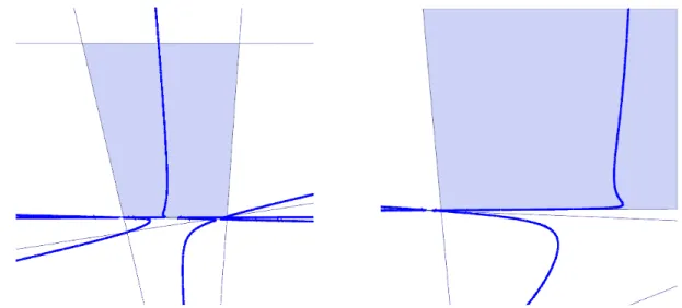
Proposition 4. The curve C is hyperbolic with respect to the point [0 : −b2 : b1]. This
means that every line inP2(
R) passing through this special point meetsC only in real points.
Proof. Any line passing through the point [0 : −b2 : b1] (except {y0 = 0}) has the form
{b1y1 +b2y2 = b0y0} for some b0 ∈ R. On such a line the objective function value of our linear program (2) is constant. See the left picture in Figure 3. We shall see in Remark 29 that, for anyb0 ∈R, the line meetsC in ds= deg(C) real points. This proves the claim. Hyperbolic curves are also known as Vinnikov curves, in light of Vinnikov’s seminal work [17, 31] relating them to semidefinite programming [23]. Semidefinite programming has been generalized to hyperbolic programming, in the work of Renegar [21] and others. A key construction in hyperbolic programming is the Renegar derivative which creates a (hy-perbolic) polynomial of degreeD−1 from any (hyperbolic) polynomial of degree D. To be
Figure 3. The degree-6 central path of a planar 7-gon in the affine charts {y0 = 1} and {y2 = 1}. Every line passing through [0 : −b2 :b1] intersects the curve in 6 real points, showing the real curve to be 3 completely-nested ovals.
precise, the Renegar derivative of a homogeneous polynomial f with respect to a point e is Ref(y) = ∂ ∂tf(y+te) |t=0.
Renegar derivatives correspond to thepolar curvesof classical algebraic geometry [11, §1.1]. The Renegar derivative off =Q
i∈I(a1iy1+a2iy2+ciy0) withe = (0,−b2, b1) is seen to be (8) Ref(y) = X i∈I (b1a1i−b2a2i) Y j∈I\{i} (a1jy1+a2jy2+cjy0) = C(y).
In words: the central curve C is the Renegar derivative, taken with respect to the cost function, of the product of the linear forms that define the convex polygon of feasible points.
The product of linear forms f = Q
i(a1iy1 +a2iy2 +ciy0) is a hyperbolic polynomial. Renegar [21] shows that if f is hyperbolic with respect to e then so is Ref. This yields a second proof for Proposition 4, stating thatC(y) is hyperbolic with respect to [0 :−b2 :b1]. Proposition 4 is visualized in Figure 3. The picture on the right is obtained from the picture on the left by a projective transformation. The point at infinity which represents the cost function is now in the center of the diagram. In this rendition, the central curve consists of three nested ovals around that point, highlighting the salient features of a Vinnikov curve. This beautiful geometry is found not just in the dual picture but also in the primal picture: Remark 5. If d = n−2 then the primal central curve lies in the plane {Ax = b}. The conditions for optimality of (1) state that the vector∇(P
ilog(xi)) = (x−11, . . . , x
−1
n ) is in the
span ofc and the rows ofA. The Zariski closure of suchxis thecentral sheet, to be studied in Section 4. Here, the central sheet is the hypersurface in Rn with defining polynomial
(9) det A1 A2 · · · An c1 c2 · · · cn x−11 x−21 · · · x−n1 · Y i∈I xi,
where Ai is the ith column of A and I ={i : { Acjj
}j∈[n]\i are linearly independent}. We
see that the degree of this hypersurface is |I| −1, so it is n−1 for generic A. Intersecting this surface with the plane {A·x=b}gives the primal central curve, which is hence a curve of degree |I| −1. The corresponding complex projective curve inP2 ={Ax=x
0b} ⊂Pn−1 is hyperbolic with respect to the point [0 :v] in Pn−1, where v spans the kernel of A
c
.
It is of importance for interior point algorithms to know the exact total curvature, formally introduced in equation (27), of the central path of a linear program (see [8, 18, 24, 30, 32]). Deza et al. [10] proved that even for d = 2 the total curvature grows linearly in n, and they conjectured that the total curvature is no more than 2πn. They named this conjecture the continuous Hirsch conjecture because of its similarity with the discrete simplex method analogue (see [9]). In Section 5 we derive general bounds for total curvature, but for plane curves, we can exploit an additional geometric feature, namely, inflection points.
Benedetti and Ded`o [4] derived a general bound for the total curvature of a real plane curve in terms of its number of inflection points and its degree. We can make this very explicit for our central path {y∗(λ) : λ∈R≥0}. Its total curvature is bounded above by (10) total curvature of the central path ≤ π·(the number of inflection points + 1). To see this, note that the Gauss map γ takes the curve into S1. As λ decreases from ∞ to 0, the cost function bTy∗(λ) strictly increases. This implies that, for any point y∗(λ)
on the curve, its image under the Gauss map has positive inner product with b, that is, bTγ(y∗(λ))≥0. Thus the image of the Gauss map is restricted to a half circle ofS1, and it cannot wrap around S1. This shows that the Gauss map can achieve a length of at most π before it must “change direction”, which happens only at inflection points of the curve.
It is known that the total number of (complex) inflection points of a plane curve of degree D is at most 3D(D−2). For real inflection points, there is an even better bound:
Proposition 6 (A classical result of Felix Klein [15]).
The number of real inflection points of a plane curve of degree D is at most D(D−2).
This provides only a quadratic bound for the total curvature of the central path in terms of its degree, but it does allow us to improve known bounds for the average total curvature. The average total curvature of the central curve of a hyperplane arrangement is the average, over all bounded regions of the arrangement, of the total curvature of the central curve in that region. Dedieuet al.[8] proved that the average total curvature in a simple arrangement (i.e. for a generic matrix A) defined by n hyperplanes in dimension d is not greater than 2πd. Whend = 2, we can use Proposition 6 to improve this bound by a factor of two. Theorem 7. The average total curvature of a central curve in the plane is at most 2π. Proof. The central curve for n general lines in R2 has degree n−1, and it consists of n−1 connected components. From the argument above and Klein’s theorem, this shows that
n−1
X
i=1
(curvature of theith component) ≤
n−1
X
i=1
π(#inflection points on the ith component + 1)
≤ π(n−1)(n−2).
Our arrangement ofn general lines has n−21 bounded regions. The average total curvature over each of these regions is therefore at most π(n−1)(n−2)/ n−21 = 2π.
To bound the curvature of just the central path, we need to bound the number of inflection points appearing on that piece of the curve. This leads to the following open problem: Question 8. What is the largest number of inflection points on a single oval of a (hyperbolic) curve of degreeD in the real plane? In particular, is this number linear in the degreeD?
It has been noted in the literature on interior point algorithms (e.g. [18, 30]) that the final stretch of the central path, shortly before reaching a non-degenerate optimal solution, is close to linear. In other words, locally, at a simple vertex of our arrangement, the central curve is well approximated by its tangent line. In closing, we wish to point out a way to see this tangent line in our derivation of the equation (7). Namely, let i and j be the indices of the two lines passing through that simple vertex. Then the equation (6) takes the following form: (11) b1a2i−b2a1i
a1iy1 +a2iy2+ci
= b1a2j−b2a1j a1jy1+a2jy2+cj
+ much smaller terms.
Dropping the small terms and clearing denominators reveals the equation of the tangent line.
3. Concepts from Matroid Theory
We have seen in the previous section that the geometry of a central curve in the plane is intimately connected to that of the underlying arrangement of constraint lines. For instance, the degree of the central curve,|I| −1, is one less than the number of constraints not parallel to the cost function. This systematic study of this kind of combinatorial information, encoded in a geometric configuration of vectors or hyperplanes, is the subject ofmatroid theory.
Matroid theory will be crucial for stating and proving our results in the rest of this paper. This section offers an exposition of the relevant concepts. Of course, there is already a well-established connection between matroid theory and linear optimization (e.g., as outlined in [16] or in oriented matroid programming [1]). Our paper sets up yet another connection. The material that follows is well-known in algebraic combinatorics, but less so in optimiza-tion, so we aim to be reasonably self-contained. Most missing details can be found in [6, 7] and the other surveys in the same series. We consider an r-dimensional linear subspaceL of the vector space Kn with its fixed standard basis. Here K is any field. Typically, L will be
given to us as the row space of an r×n-matrix. The kernel of that matrix is denoted byL⊥.
This is a subspace of dimension n−r in Kn. We write x1, . . . , xn for the restriction of the
standard coordinates on Kn to the subspace L, and s1, . . . , sn for their restriction to L⊥.
The two subspaces L andL⊥ specify a dual pair of matroids, denotedM(L) and M(L⊥),
on the set [n] ={1, . . . , n}. The matroidM(L) has rankr and its dualM(L⊥) = M(L)∗ has
rank n−r. We now define the first matroid M =M(L) by way of its independent sets. A subsetI of [n] isindependent inM if the linear forms in{xi :i∈I}are linearly independent
onL. Maximal independent sets are calledbases. These all have cardinalityr. A subsetI is
dependentif it is not independent. It is acircuitif it is minimally dependent. For example, if K is an infinite field andL is a general subspace then we get theuniform matroidM =Ur,n
whose bases are all r-subsets in [n] and whose circuits are all (r+ 1)-subsets of [n]. The bases of the dual matroid M∗ are the complementary sets [n]\B whereB is any basis ofM. The most prominent invariant in the theory of matroids is the Tutte polynomial (see [7]). To define this, we assume the usual order 1<2<· · ·< non the ground set [n], but it turns out that the definition is independent of which ordering is chosen. LetB be a basis ofM and consider any elementp∈[n]\B. Then the setB∪ {p}is dependent, and it contains a unique circuitC. The circuit C containsp. We say that pisexternally active forB if pis the least
element inC, in symbols, p= min(C). Similarly, an elementp∈B is calledinternally active
if pis the least element that completes the independent setB\{p}to a basis of the matroid. Let ia(B, w) and ea(B, w) denote the number of internally and externally active elements associated to the basisB. Then theTutte polynomial of M is the bivariate polynomial
TM(x, y) =
X
B∈B(M)
xia(B,w)yea(B,w).
It satisfies the duality relation TM∗(x, y) =TM(y, x); see [7, Proposition 6.2.4].
An important specialization of the Tutte polynomial is the characteristic polynomial
χM(t) = (−1)r·TM(1−t,0).
This univariate polynomial plays a key role in the enumerative theory of hyperplane arrange-ments [33]. The characteristic polynomial can be rewritten in terms of the lattice of flats of the matroid. Its coefficients are values of theM¨obius function λM. An important number for
us is the M¨obius invariant [7, Eq. (6.21)]. It is defined in terms of the following evaluations: (12) µ(M) = (−1)r·TM(1,0) = χM(0) = λM(∅,[n]).
Throughout this paper we use the absolute value|µ(M)|and call it theM¨obius numberofM. In algebraic combinatorics, one regards the independent sets of the matroidM as the faces in a simplicial complex of dimensionr−1. We write fi(M) for the number of i-dimensional
faces of thisindependence complex of M. Equivalently, fi(M) is the number of independent
sets of cardinality i+ 1. By [6, Proposition 7.4.7 (i)], the (reduced) Euler characteristic,
−1 +f0(M)−f1(M) +· · ·+fr−1(M), of the independence complex of a matroidM coincides up to sign with the M¨obius invariant of the dual matroid M∗:
(13) µ(M∗) = (−1)r−1 −1 + r−1 X i=0 (−1)ifi(M) ! .
We apply this to compute the M¨obius number of the uniform matroid M =Ur,n as follows:
(14) |µ(Ur,n)| = |µ(Un−r,n∗ )| = n−r−1 X i=−1 (−1)n−r+i+1 n i+ 1 = n−1 r−1 . This binomial coefficient is an upper bound on |µ(M)| for any rankr matroid M on [n].
A useful characterization of the M¨obius number involves another simplicial complex on [n] associated with the matroid M. As before, we fix the standard ordering 1<2<· · · < n of [n], but any other ordering will do as well. A broken circuit of M is any subset of [n] of the form C\{min(C)} where C is a circuit. The broken circuit complex of M is the simplicial complex Br(M) whose minimal non-faces are the broken circuits. Hence, a subset of [n] is a face of Br(M) if it does not contain any broken circuit. It is known that Br(M) is a shellable simplicial complex of dimensionr−1 (see Theorem 7.4.3 in [6]). We can recover the M¨obius number of M (not that of M∗) as follows. Let fi =fi(Br(M)) denote the number
of i-dimensional faces of the broken circuit complex Br(M). The corresponding h-vector (h0, h1, . . . , hr−1) can be read off from any shelling (cf. [6, §7.2] and [25, §2]). It satisfies
(15) r−1 X i=0 fi−1zi (1−z)i = h0+h1z+h2z2+· · ·+hr−1zr−1 (1−z)r .
The relation between f-vector and h-vector holds for any simplicial complex [25]. The next identity follows from [6, Eq. (7.15)] and the discussion on shelling polynomials in [6, §7.2]: (16) h0+h1z+h2z2+· · ·+hr−1zr−1 = zr·TM(1/z,0).
The rational function (15) is the Hilbert series (see [25]) of the Stanley-Reisner ring of the broken circuit complex Br(M). The defining ideal of the Stanley-Reisner ring is generated by the monomials Q
i∈C\{min(C)}xi representing broken circuits. Proudfoot and Speyer [20]
constructed abroken circuit ring, which is the quotient ofK[x1, . . . , xn] modulo a prime ideal
whose initial ideal is precisely this monomial ideal. Hence (15) is also the Hilbert series of the ring in [20]. In particular, the M¨obius number is the common degree of both rings: (17) |µ(M)| = h0 +h1+h2+· · ·+hr−1.
This result is obtained from setting z = 1 in (16) and applying the identity (12).
The M¨obius number is important to us because it computes the degree of the central curve of the primal linear program (1). See Theorem 12 below. The matroid we need there has rankr =d+ 1 and it is denoted MA,c. The correspondingr-dimensional vector subspace of Kn is denoted L
A,c. It is spanned by the rows of A and the vector c. We use the notation (18) |µ(A,c)| := |µ(MA,c)| = |µ(M(LA,c))|.
The constraint matrixA has real entries and it hasncolumns and rankd. We writeQ(A) for the subfield of R generated by the entries of A. In Section 4 we shall assume that the coordinatesbi andcj of the right hand sideband the cost vectorcare algebraically
indepen-dent over Q(A), and we work over the rational function field K =Q(A)(b,c) generated by these coordinates. This will ensure that all our algebraic results derived remain valid under almost all other specializations K →R of these coordinates to the field of real numbers.
We now present a geometric interpretation of the M¨obius number |µ(M)| in terms of hy-perplane arrangements. The arrangements we discuss often appear in linear programming, in the context of pivoting algorithms, such as the criss-cross method [12]. Fix anyr-dimensional linear subspace L ⊂ Rn and the associated rank r matroid M =M(L). For our particular
application in Section 4, we would take r =d+ 1, L=LA,c and M =MA,c.
Letu be a generic vector in Rn and consider the (n−r)-dimensional affine space L⊥+u
of Rn. The equations xi = 0 define n hyperplanes in this affine space. These hyperplanes
do not meet in a common point. In fact, the resulting arrangement {xi = 0}i∈[n] in L⊥+u is simple, which means that no point lies on more than n−r of the n hyperplanes. The vertices of this hyperplane arrangement are in bijection with the bases of the matroid M. The complements of the hyperplanes are convex polyhedra; they are the regions of the arrangement. Each region is either bounded or unbounded, and we are interested in the bounded regions. These bounded regions are the feasibility regions for the linear programs with various sign restrictions on the variables xi (one of the regions is xi ≥ 0 for all i).
Proposition 6.6.2 in [7], which is based on results of Zaslavsky [33], establishes the following: (19) |µ(M)| = # bounded regions of the hyperplane arrangement {xi = 0}i∈[n] in L⊥+u.
ForM =MA,c, the affine linear spaceL⊥+uis cut out by the equations Ac
x= Acu. It is instructive to examine equation (19) for the case of the uniform matroid M =Ur,n. Here
we are given n general hyperplanes through the origin inRn−r, and we replace each of them by a random parallel translate. The resulting arrangement of n affine hyperplanes in Rn−r creates precisely n−r−11 bounded regions, as promised by the conjunction of (14) and (19).
For example, if r = 1 then |µ(U1,n)| = 1, since n hyperplanes in Rn−1 can create only one bounded region. At the other hand, if r = n−1 then our n affine hyperplanes are just n points on a line and these will create |µ(Un−1,n)|=n−1 bounded line segments.
For a relevant instance of the latter case consider Example 2, with A the displayed 5× 6-matrix of rankd= 4, or the instance in Figure 3. Here,n = 6,r=d+1 = 5, andMA,c=U5,6 is the uniform matroid. Its M¨obius number equals |µ(A,c)|=|µ(U5,6)|= 5. This number 5 counts the bounded segments on the vertical red line on the left in Figure 3. Note that the relevant matroid for Example 2 is not, as one might expect, the graphic matroid ofK2,3. For higher-dimensional problems the matroids MA,c we encounter are typically non-uniform.
4. Equations defining the central curve
In this section we determine the prime ideal of the central curve of the primal linear program (1). As a consequence we obtain explicit formulas for the degree, genus and Hilbert function of the projective closure of the primal central curve. These results resolve the problem stated by Bayer and Lagarias at the end of [3,§11]. Let LA,c be the subspace ofKn spanned by the rows of A and the vector c. Our ground field is K =Q(A)(b,c) as above. We define the central sheetto be the coordinate-wise reciprocalL−1
A,cof that linear subspace. In precise terms, we define L−1
A,c to be the Zariski closure in the affine space Cn of the set
(20) 1 u1 , 1 u2 , . . . , 1 un ∈Cn : (u 1, u2, . . . , un)∈ LA,c and ui 6= 0 for i= 1, . . . , n . Lemma 9. The Zariski closure of the primal central path {x∗(λ) : λ∈R≥0} is equal to the
intersection of the central sheet L−1
A,c with the affine-linear subspace defined by A·x=b.
Proof. We eliminates,yandλfrom the equations ATy−s=c and x
isi =λ as follows. We
first replace the coordinates ofs bysi =λ/xi. The linear system becomes ATy−λx−1 =c.
This condition means that x−1 = (1
x1, . . . ,
1
xn) lies in the linear space LA,c spanned byc and
the rows of A. The result of the elimination says that xlies in the central sheet L−1
A,c. The linear space {Ax = b} has dimension n −d, and we write IA,b for its linear ideal. The central sheet L−1
A,c is an irreducible variety of dimension d+ 1, and we writeJA,c for its prime ideal. Both IA,b and JA,c are ideals inK[x1, . . . , xn]. We argue the following is true:
Lemma 10. The prime ideal of polynomials that vanish on the central curve C is IA,b+JA,c.
The degree of both C and the central sheet L−A,1c coincides with the M¨obius number |µ(A,c)|. Proof. The intersection of the linear space {Ax = b} with the central sheet is the variety of the ideal IA,b +JA,c. This ideal is prime because b and c are generic over Q(A). The intersection is the central curve. In Proposition 11 we show that the degree of the central sheet is |µ(A,c)|, so here it only remains to show that this is the degree of the central curve as well. For a generic vector (b, c0)∈Rd+1, we consider the hyperplane arrangement induced by {xi = 0} in the affine space { Ac
x = c0b}. The number of bounded regions of this hyperplane arrangement equals the M¨obius number |µ(A,c)|, as seen in (19).
Note that |µ(A,c)| does not depend on c, since this vector is generic over Q(A). Each of the |µ(A,c)| bounded regions in the (n−d−1)-dimensional affine space { Ac
x = c0b}
contains a unique point maximizing P
region. Each such analytic center lies inL−A,1c, and thus on the central curve. This shows that the intersection of the central curve with the plane {cTx=c
0} contains |µ(A,c)| points. B´ezout’s Theorem implies that the degree of a variety V ⊂Cn is an upper bound for the
degree of its intersectionV∩Hwith an affine-linear spaceH, provided thatn+dim(V ∩H) = dim(V) + dim(H). We use this theorem for two inequalities; first, that the degree of L−1
A,c bounds the degree of the central curveC, and second that the degree ofC bounds the number of its intersection points with{c·x=c0}. To summarize, we have shown:
|µ(A,c)| ≤ #(C ∩ {c·x=c0}) ≤ deg(C) ≤ deg(L−A,1c) = |µ(A,c)|.
From this we conclude that|µ(A,c)|is the degree of the primal central curve C. At this point we are left with the problem of computing the minimal generators and the degree of the homogeneous ideal JA,c. Luckily, this has already been done for us in the
literature through matroid tools. The following proposition was proved by Proudfoot and Speyer [20] and it refines an earlier result of Terao [27]. See also [5]. The paper [26] indicates how our results can be extended from linear programming to semidefinite programming. Proposition 11 (Proudfoot-Speyer [20]). The degree of the central sheet L−1
A,c, regarded as
a variety in complex projective space, coincides with the M¨obius number |µ(A,c)|. Its prime idealJA,cis generated by a universal Gr¨obner basis consisting of all homogeneous polynomials
(21) X i∈supp(v) vi· Y j∈supp(v)\{i} xj, where P
vixi runs over non-zero linear forms of minimal support that vanish on LA,c.
Proof. The construction in [20] associates the ringK[x1, . . . , xn]/JA,c to the linear subspace
LA,c ofKn. Theorem 4 of [20] says that the homogeneous polynomials (21) form a universal Gr¨obner bases forJA,c. As argued in [20, Lemma 2], this means that the ring degenerates to the Stanley-Reisner ring of the broken circuit complex Br(MA,c). Hence, by our discussion in Section 3, or by [20, Prop. 7], the Hilbert series ofK[x1, . . . , xn]/JA,c is the rational function (15), and the degree of JA,c equals |µ(A,c)| as seen in (17). The ideal JA,c is radical, since its initial ideal is square-free, and hence it is prime because its varietyL−1
A,cis irreducible. The polynomials in (21) correspond to the circuits of the matroid MA,c. There is at most one circuit contained in each (d+ 2)-subset of{x1, . . . , xn}, so their number is at most d+2n
. If the matrix A is generic then MA,c is uniform and, by (14), its M¨obius number equals
|µ(A,c)| = n−1 d .
For arbitrary matricesA, this binomial coefficient furnishes an upper bound on the M¨obius number |µ(A,c)|. We are now prepared to conclude with the main theorem of this section. The analogous equations for the dual central curve are given in Proposition 22 in Section 6. Theorem 12. The degree of the primal central path of (1) is the M¨obius number |µ(A,c)| and is hence at most n−d1. The prime ideal of polynomials that vanish on the primal central path is generated by the circuit polynomials (21) and the d linear polynomials in Ax−b. Proof. This is an immediate consequence of Lemmas 9 and 10 and Proposition 11.
It is convenient to write the circuit equations (21) in the following determinantal repre-sentation. Suppose that A has format d×n and its rows are linearly independent. Then the linear forms of minimal support that vanish onLA,c are the (d+ 2)×(d+ 2)-minors of the (d+ 2)×n matrix
A
c x
. This gives the following concise description of our prime idealJA,c:
(22) JA,c = Inum,d+2 A c x−1
wherex−1 = (x−11, . . . , xn−1) and the operatorInum,d+2 extracts the numerators of the (d+2)× (d+2)-minors of the matrix. Note that there are d+2n
such minors but they need not be distinct. For example, the generator of JA,c coming from the leftmost minor equals
det A1 A2 . . . Ad+2 c1 c2 . . . cd+2 x−11 x−21 . . . x−d+21 · Y i∈I xi,
where I is the lexicographically earliest circuit of the matroid MA,c.
Example 13. Letd= 4, n = 6 andA the matrix in Example 2. The linear ideal is IA,b = hx1+x2+x3−b1, x4+x5+x6−b2, x1+x4 −b3, x2+x5−b4i. The central sheet L−1
A,c is the quintic hypersurface whose defining polynomial is
(23) fA,c(x) = det 1 1 1 0 0 0 0 0 0 1 1 1 1 0 0 1 0 0 0 1 0 0 1 0 c1 c2 c3 c4 c5 c6 x−11 x−21 x−31 x−41 x−51 x−61 ·x1x2x3x4x5x6.
The primal central curve is the plane quintic defined by the idealIA,b+hfA,ci. This ideal is prime for general choices of b and c. However, this may fail for special values: the quintic on the left in Figure 1 is irreducible but that on the right decomposes into a quartic and a line. For a concrete numerical example we set b1 =b2 = 3 and b3 = b4 =b5 = 2. Then the transportation polygon P is the regular hexagon depicted in Figure 1. Its vertices are (24) 0 1 2 2 1 0 , 0 2 1 2 0 1 , 1 0 2 1 2 0 , 1 2 0 1 0 2 , 2 0 1 0 2 1 , 2 1 0 0 1 2 . Consider the two transportation problems (1) given by c=
0 0 0 0 1 3 and c0 = 0 0 0 0 1 2 .
In both cases, the last matrix in (24) is the unique optimal solution. Modulo the linear ideal IA,b we can write the quintics fA,c and fA,c0 as polynomials in only two variables x1 and x2:
fA,c = 3x41x2+ 5x31x22−2x1x42−3x41−22x31x2−15x21x22+ 8x1x32+ 2x42 +18x3 1+ 45x21x2−12x32−33x21−22x1x2+ 22x22+ 18x1−12x2, fA,c0 = (x2−1)·(2x 4 1+ 4x31x2 +x21x22−x1x32−12x31−14x21x2 +x1x22 +x32+ 22x21+ 10x1x2−5x22−12x1+ 6x2).
Both quintics pass through all intersection points of the arrangement of six lines. The cost matrix c exemplifies the generic behavior, when the quintic curve is irreducible. On the other hand, the central path forcis a segment on the horizontal linex2 = 1 in Figure 1.
In the remainder of this section we consider the question of what happens to the central sheet, and hence to the central path, when the cost function c degenerates to one of the unit vectors ei. Geometrically this means that the cost vector becomes normal to one of the
constraint hyperplanes, and the curve reflects this by breaking into irreducible components. What follows is independent of the rest of the paper and can be skipped upon first reading. To set up our degeneration in proper algebraic terms, we work over the field K{{t}} of Puiseux series over the field K = Q(A)(b,c) that was used above. The field K{{t}} comes with a naturalt-adic valuation. Passing to the special fiber represents the process of letting the parameter t tend to 0. Our cost vector c has its coordinates in the Puiseux series field: (25) c = tw1, tw2, . . . , twn−1,1
Here w1 > w2 >· · ·> wn−1 >0 are any rational numbers. We are interested in the special fiber of the central sheet L−1
A,c. This represents the limit of the central sheet as t approaches 0. This induces a degeneration of the central curve L−1
A,c ∩ {Ax=b}. We wish to see how, in that limit, the central curve breaks into irreducible curves in the affine space {Ax=b}.
The ideal defining the special fiber of JA,c is denoted in(JA,c) = JA,c|t=0. By a combi-natorial argument as in [20], the maximal minors in (22) have the Gr¨obner basis property for this degeneration. Hence we obtain the prime ideal of the flat family by simply dividing each such minor by a non-negative power oft. This observation implies the following result: Theorem 14. The central sheet L−1
A,c degenerates into a reduced union of central sheets of
smaller linear programming instances. More precisely, the ideal in(JA,c) is radical, and it
has the following representation as an intersection of ideals that are prime whenAis generic:
(26) in(JA,c) = n−1 \ i=d Inum,d+1 A1 A2 · · · Ai x−11 x−21 · · · x−i 1 + hxi+2, xi+3, . . . , xni
Proof sketch. The Gr¨obner basis property says that in(JA,c) is generated by the polynomials obtained from the maximal minors of (22) by dividing by powers of t and then setting t to zero. The resulting polynomials factor, and this factorization shows that they lie in each of the ideals on the right hand side of (26). Conversely, each element in the product of the ideals on the right hand side is seen to lie in in(JA,c). To complete the proof, it then suffices to note that in(JA,c) is radical because its generators form a square-free Gr¨obner basis. Example 15. Let n = 6 and d = 3. The matrix A might represent the three-dimensional Klee-Minty cube. The decomposition of the initial ideal in (26) has three components: in(JA,c) = hx5, x6i ∩ hdet x1A1 x2A2 x3A3 x4A4 1 1 1 1 , x6i ∩ Inum,4 A1 A2 A3 A4 A5 x1−1 x−21 x3−1 x−41 x−51 . For general A, the ideal JA,c defines an irreducible curve of degree 10, namely the central path, in each of the 3-planes {Ax = b}. The three curves in its degeneration above are irreducible of degrees 1, 3 and 6 respectively. The first is one of the lines in the arrangement of six facet planes, the second curve is the central path inside the facet defined by x6 = 0, and the last curve is the central path of the polytope obtained by removing that facet. In general, we can visualize the degenerated central path in the following geometric fashion. We first flow from the analytic center of the polytope to the analytic center of its last facet. Then we iterate and flow from the analytic center of the facet to the analytic center of its last facet, which is a ridge of the original polytope. Then we continue inside that ridge, etc.
5. The Gauss Curve of the Central Path
The total curvature of the central path is an important quantity for the estimation of the running time of interior point methods in linear programming. In this section we relate the algebraic framework developed so far to the problem of bounding the total curvature. The relevant geometry was pioneered by Dedieu, Malajovich and Shub [8]. Following their approach, we consider the Gauss curveassociated with the primal central path. The Gauss curve is the image of the central curve under the Gauss map, and its arc length is precisely the total curvature of the central path. Moreover, the arc length of the Gauss curve can be bounded in terms of its degree. An estimate of that degree, via the multihomogeneous B´ezout Theorem, was the workhorse in [8]. Our main result here is a much more precise bound, in terms of matroid invariants, for the degree of the Gauss curve of the primal central curve. As a corollary we obtain a new upper bound on the total curvature of that central curve.
We begin our investigation by reviewing definitions from elementary differential geometry. Consider an arbitrary curve [a, b] → Rn, t 7→ f(t), whose parameterization is twice
differ-entiable and whose derivative f0(t) is a non-zero vector for all parameter values t ∈ [a, b]. This curve has an associated Gauss map into the unit sphere Sm−1, which is defined as
γ : [a, b]→Sm−1, t 7→ f
0(t)
||f0(t)||.
The imageγ =γ([a, b]) of the Gauss map inSm−1is called theGauss curveof the given curve f. In our situation, the curvef is algebraic, with known defining polynomial equations, and it makes sense to consider theprojective Gauss curve in complex projective space Pm−1. By this we mean the Zariski closure of the image of the Gauss curve under the double-cover map Sm−1 →
Pm−1. If m = 2, so that C is a non-linear plane curve, then the Gauss curve traces out several arcs on the unit curve S1, and the projective Gauss curve is the entire projective line P1. Here, the line
P1 comes with a natural multiplicity, to be derived in Example 19. If m= 3 then the Gauss curve lies on the unit sphere S2 and the projective Gauss curve lives in the projective planeP2. Since a curve in 3-space typically has parallel tangent lines, the Gauss curve is here expected to have singularities, even if f is a smooth curve.
Thetotal curvature K of our curvef is defined to be the arc length of its associated Gauss curve γ; see [8,§3]. This quantity admits the following expression as an integral:
(27) K :=
Z b
a
||dγ(t)
dt ||dt.
The total curvature of the central path is a very interesting number for linear programming. The degree of the Gauss curve γ(t) is defined as the maximum number of intersection points, counting multiplicities, with any hyperplane in Rm, or equivalently, with any equa-tor in Sm−1. This (geometric) degree is bounded above by the (algebraic) degree of the projective Gauss curve in Pm−1. The latter can be computed exactly, from any polynomial representation of C, using standard methods of computer algebra. Throughout this section, bydegree we mean the degree of the image of curve in Pm−1 multiplied by the degree of the map that takes C onto γ(C). From now on we use the notation deg(γ(C)) for that number. Proposition 16. [8, Corollary 4.3] The total curvature of any real algebraic curve C in Rm is bounded above by π times the degree of its projective Gauss curve in Pm−1. In symbols,
We now present our main result in this section, which concerns the degree of the projective Gauss curve γ(C), when C is the central curve of a linear program in primal formulation. As before, A is an arbitrary real matrix of rank d havingn columns, but the cost vector c and the right hand side b are generic over Q(A). The curve C lives in an (n−d)-dimensional affine subspace of Rn, which we identify with
Rn−d, so that γ(C) is a curve in Pn−d−1. Let MA,c denote the matroid of rank d+ 1 on the ground set [n] = {1, . . . , n} associated with the matrix Ac. We write (h0, h1, ...., hd) for the h-vector of the broken circuit complex
of MA,c, as defined in (15). In the generic case, when MA,c=Ud+1,n is the uniform matroid,
the maximal simplices in Br(MA,c) are {1, j1, . . . , jd} where 2 ≤j1 < · · ·< jd ≤n. In that
case, the coordinates of the h-vector are found to be hi = n−d+ii−2
. For special matrices A, this simplicial complex gets replaced by a pure shellable subcomplex of the same dimension, so the h-vector (weakly) decreases in each entry. Hence, the following always holds:
(28) hi ≤ n−d+i−2 i for i= 0,1, . . . , d.
As indicated, this inequality holds with equality when MA,c is the uniform matroid.
Theorem 17. The degree of the projective Gauss curve of the primal central curveC satisfies
(29) deg(γ(C)) ≤ 2·
d
X
i=1 i·hi.
In particular, we have the following upper bound which is tight for generic matrices A:
(30) deg(γ(C)) ≤ 2·(n−d−1)· n−1 d−1 .
The difference between the bound in (29) and the degree ofγ(C) can be explained in terms of singularities the curve C may have on the hyperplane at infinity. The relevant algebraic geometry will be seen in the proof of Theorem 17, which we shall present after an example. Example 18. Letd= 3 and n= 6. We first assume that A is a generic 3×6-matrix. The arrangement of six facet planes creates 10 bounded regions. The primal central curveC has degree 6−31= 10. It passes through the 63 = 20 vertices of the arrangements. In-between it visits the 10 analytic centers of the bounded regions. Here the curve C is smooth and its genus is 11. This number is seen from the formula (33) below. The corresponding Gauss curve in the projective plane has degree 2·10 + 2·genus(C)−2 = 40, as given by the right hand side of (30). Hence the total curvature of the central curveC is bounded above by 40π. Next we consider the classical Klee-Minty cube in 3-space. It is given by the constraints (31) 0≤x≤1, x≤y≤1−x, and y≤z ≤1−y.
In its primal formulation, the general linear program over this polytope is given by the matrix
A c = 1 1 0 0 0 0 2 0 1 1 0 0 22 0 2 0 1 1 c1 c2 c3 c4 c5 c6 .
Here is a small positive real constant. The above 4×6-matrix is not generic, and its associated matroid MA,c is not uniform. It has exactly one non-basis, and so the h-vector equals (h0, h1, h2, h3) = (1,2,3,3). The central curve C has degree P3
coordinates used in (31), the curve is defined by the 5×5-minors of the 5×6-matrix which is obtained from the 4×6-matrix Acby adding one row consisting of reciprocal facet equations:
x−1, (1−x)−1, (y−x)−1, (1−y−x)−1, (z−y)−1, (1−z−y)−1.
According to Theorem 17, the degree of the Gauss curve γ(C) in P2 is bounded above by 2P3
i=1i·hi = 34. A computation using Macaulay2 [13] reveals that degree(γ(C)) = 32. Proof of Theorem 17. For the proof we shall use the generalized Pl¨ucker formula for curves: (32) deg(γ(C)) = 2·deg(C) + 2·genus(C)−2−κ.
The formula in (32) is obtained from [19, Thm. (3.2)] by settingm= 1 or from [14, Eq. (4.26)] by setting k = 0. The quantityκ is a non-negative integer and it measures the singularities of the curve C. We have κ = 0 whenever C is a smooth curve, and this happens in our application when MA,c is the uniform matroid. In general, we may have singularities at infinity because here the real affine curve C has to be replaced by its closure in complex projective space Pn−d, which is the projectivization of the affine space defined by Ax = b. The degree and genus on the right hand side of (32) refer to that projective curve in Pn−d.
The references above actually give the degree of the tangent developable of the projective curveC, but we see that this equals the degree of the Gauss curve. The tangent developable is the surface obtained by taking the union of all tangent lines at points in C. The pro-jective Gauss curve γ(C) is obtained from the tangent developable by intersecting it with a hyperplane, namely, the hyperplane at infinity, representing the directions of lines.
In the formula (32), the symbol genus(C) refers to the arithmetic genus of the curve. We shall now compute this arithmetic genus for primal central curve C. For this we use the formula for the Hilbert series of the central sheet due to Terao, in Theorem 1.2 on page 551 of [27]. See the recent work of Berget [5] for a nice proof of a more general statement.
As seen in the proof of Proposition 11, the Hilbert series of its coordinate ring equals h0+h1z+h2z2+· · ·+hdzd
(1−z)d+2 .
The central curve C is obtained from the central sheet by intersection with a general linear subspace of dimension n−d. The (projective closure of the) central sheet is arithmetically Cohen-Macaulay since it has a flat degeneration to a shellable simplicial complex, as shown by Proudfoot and Speyer [20]. We conclude that the Hilbert series of the central curve C is
h0+h1z+h2z2+· · ·+hdzd (1−z)2 = X m≥d ( d X i=0 hi)·m + d X j=0 (1−j)hj zm + O(zd−1).
The parenthesized expression is the Hilbert polynomial of the projective curveC. The degree ofC is the coefficient ofm, and we recover our result relating the degree and M¨obius number:
degree(C) = |µ(A,c)| =
d
X
i=0 hi.
The arithmetic genus of the curveC is one minus the constant term of its Hilbert polynomial:
(33) genus(C) = 1−
d
X
j=0
We now see that our assertion (29) follows directly from the generalized Pl¨ucker formula (32). When d and n are fixed, then the degree and genus of C are maximal when the matrix A is generic. In this case, hi equals the right hand side of (28), and we need to sum these
binomial coefficients times two. Hence, our second assertion (30) follows from the identify
d X i=0 i· n−d+i−2 i = (n−d−1)· n−1 d−1 .
This complete the proof of Theorem 17.
Example 19. Let d = n−2 and suppose A is generic. Here, the primal central curve C
is a plane curve. Our h-vector equals (1,1, ...,1). Theorem 17 reveals that the degree of C
is d+ 1 and the genus of C is d2
. In this case, the Gauss curve γ(C) is the projective line P1, but regarded with multiplicity deg(γ(C)) = (d+ 1)d. This number is the degree of the projectively dual curve C∨. The identity (32) specializes to the Pl¨ucker formula for plane
curves, which expresses the degree ofC∨ in terms of the degree and the singularities ofC.
In the next section we shall establish a dictionary that translates between the primal and the dual central curve. As we shall see, all our results hold essentially verbatim for the dual central curves. In particular, the discussion in Example 19 above applies also to the situation of Section 2, where we discussed dual central curves that live in the plane (d= 2), such as: Example 20. Consider the DTZ snake in Figure 2. The curve shown there has degree 4 and its projective closureC is smooth inP2. So, we have deg(γ(C)) = 12, and Proposition 16 would give the upper bound 12π on the total curvature of the full central curve inR2. We close this section by showing how to compute the Gauss curve for a non-planar instance. Example 21. Let n = 5, d = 2 and A =
1 1 1 1 1 0 1 2 3 4
. The primal central curve has degree 6 and its equations are obtained by clearing denominators in the 4×4-minors of
1 1 1 1 1 0 1 2 3 4 c1 c2 c3 c4 c5 (x−g1)−1 (−2x+y−g2)−1 (x−2y+z−g3)−1 (y−2z−g4)−1 (z−g5)−1 .
Theci andgj are random constants representing the cost function and right hand side of (1).
To be precise, the vectorg = (g1, g2, g3, g4, g5)T satisfies Ag=b as in Section 6. Writing I
for the ideal of these polynomials, the following one-line command in the computer algebra system Macaulay2 [13] computes the defining polynomial of the Gauss curve in P2:
eliminate({x,y,z},I+minors(1,matrix{{u,v,w}}*diff(matrix{{x},{y},{z}},gens I)))
The output is a homogeneous polynomial of degree 16 in the coordinatesu, v, w onP2. Note that deg(γ(C)) = 16 is consistent with Theorem 17 becauseh= (h0, h1, h2) = (1,2,3).
6. Global Geometry of the Central Curve
In this section we return to the central path in its original primal-dual formulation, and we study its geometric properties. We shall study how the central curve connects the vertices of the hyperplane arrangement with the analytic centers of its bounded regions. This picture behaves well under duality, as the vertices of the two arrangements are in natural bijection.
We begin by offering an algebraic representation of the primal-dual central curve that is more symmetric than that given in the Introduction. Let LA denote the row space of the
matrix A and L⊥
A its orthogonal complement in Rn. We also fix a vector g ∈ Rn such that
Ag = b. By eliminating y from the system (5) in Theorem 1, we see that the primal-dual central path (x∗(λ),s∗(λ)) has the following description that is symmetric under duality: (34) x∈ L⊥A+g, s∈ LA+c and x1s1 =x2s2 =· · ·=xnsn=λ.
The implicit (i.e. λ-free) representation of the primal-dual central curve is simply obtained by erasing the very last equality “=λ” in (34). Its prime ideal is generated by the quadrics xisi−xjsj and the affine-linear equations definingL⊥A+g inx-space andLA+cins-space.
The symmetric description of the central path in (34) lets us write down the statements from Section 4 for the dual version. For example, we derive equations for the dual central curve in s-space or y-space as follows. Let B be any (n−d)×n matrix whose rows span the kernel of A. In symbols, LB = L⊥A. The (dual) central curve in s-space is obtained by
intersecting thed-dimensional affine space LA+c ={s∈Rn : Bs=Bc} with the central
sheet L−1
B,g (20). To obtain the central curve in y-space, we substitute si =Pjd=1ajiyj+ci
in the equations defining L−1
B,g. This gives dual formulations of Theorems 12 and 17:
Corollary 22. The degree of the dual central curve of (2) equals the M¨obius number|µ(B,g)| and is hence at most n−d−11. The prime ideal of polynomials that vanish on the central path is generated by the circuit polynomials (21), but now associated with the space generated by the rows of B and the vector g, and the n−d linear equations in s given by Bs=Bc.
Corollary 23. The degree deg(γ(C)) of the Gauss image of the dual central curve C is at most P
ii·hi, where h=h(Br(MB,g)). This implies the bound deg(γ(C))≤2·(d−1)· n−1
d
.
In algebraic geometry, it is more natural to replace each of the affine spaces in (34) by a complex projective space Pn, and to study the closure C of the central curve in
Pn×Pn. Algebraically, we use homogeneous coordinates [x0 : x1 : · · · : xn] and [s0 : s1 : · · · : sn].
Writingx and s for the corresponding column vectors of lengthn+ 1, we represent
L⊥A+g by {x∈Pn: (−b, A)·x= 0} and L
A+c by {s∈Pn: (−Bc, B)·s= 0}.
The projective primal-dual central curve C is an irreducible curve in Pn × Pn. Its
bi-homogeneous prime ideal in K[x0, x1, . . . , xn, s0, s1, . . . , sn] can be computed by the process
of saturation. Namely, we compute it as the saturation with respect to hx0s0i of the ideal generated by the above linear forms together with the bi-homogeneous forms xisi−xjsj.
Example 24. Let d = 2, n = 4. Fix 2×4-matrices A = (aij) and B = (bij) such that
LB =L⊥A. We start with the ideal J in K[x0, . . . , x4, s0, . . . , s4] generated by a11(x1−g1x0) +a12(x2−g2x0) +a13(x3−g3x0) +a14(x4−g4x0), a21(x1−g1x0) +a22(x2−g2x0) +a23(x3−g3x0) +a24(x4−g4x0), b11(s1−c1s0) +b12(s2−c2s0) +b13(s3−c3s0) +b14(s4−c4s0), b21(s1−g1s0) +b22(s2−c2s0) +b23(s3−c3s0) +b24(s4−c4s0),
s1x1−s2x2, s2x2−s3x3, s3x3−s4x4.
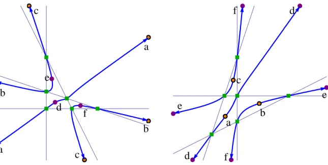
The central curve C is irreducible in P4 ×P4. It has degree (3,3) unless A is very special. The prime ideal of C is computed as the saturation (J : hx0s0i∞). We find that this ideal has two minimal generators in addition to the seven above. These are cubic polynomials in xand ins, which define the primal and dual central curves. They are shown in Figure 4.
Returning to the general case, the primal-dual curveC is always irreducible, by definition. Since it lives in Pn×
Pn, its degree is now a pair of integers (dx, ds). These two integers can be defined geometrically: dx is the number of solutions of a general equation Pni=0αixi = 0
on the curveC, and ds is the number of solutions of a general equation Pin=0βisi = 0 onC.
Corollary 25. Let c and g be generic vectors in Rn and let (d
x, ds) be the degree of the
projective primal-dual central curve C ⊂ Pn×
Pn. This degree is given by our two M¨obius
numbers, namely dx=|µ(A,c)| and ds =|µ(B,g)|. These numbers are defined in (18).
Proof. The projection from the primal-dual central curve onto its image in eitherx-space or s-space is birational. For instance, if x is a general point on the primal central curve then the corresponding pointsis uniquely obtained by solving the linear equationsxisi =xjsj on
LA+c. Likewise, given a general point son the dual central curve we can recover the unique
x such that (x,s)∈ C. This implies that the intersections in Pn×
Pn that define dx and ds are equivalent to intersecting the primal or dual central curve with a general hyperplane in Pn, and the number of points on that intersection is the respective M¨obius number. Next we discuss the geometry of this correspondence between the primal and dual curves at their special points, namely vertices and analytic centers of the relevant hyperplane ar-rangements. These special points are given by intersectingC with certain bilinear equations. The sum of our two M¨obius numbers, dx+ds, is the number of solutions of a general bilinear equation P
i,jγijxisj = 0 on the primal-dual central curve C. Two special choices of such
bilinear equations are of particular interest to us, namely, the bilinear equation x0s0 = 0 and the bilinear equation xisi = 0 for any i ≥ 1. Note that the choice of the index i does
not matter for the second equation because xisi =xjsj holds on the curve.
Let us first observe what happens in Pn×
Pn when the parameter λ becomes 0. The corresponding points on the primal-dual curveC are found by solving the equationsx1s1 = 0 onC. Its points are the solutions of the nequations x1s1 =x2s2 =· · ·=xnsn = 0 on the
n-dimensional subvariety (L⊥
A+g)×(LA+c) of Pn×Pn. This intersection now contains many
points in the product of affine spaces, away from the hyperplanes {x0 = 0} and {s0 = 0}. We find the points by solving the linear equations xi1 = · · · = xid = 0 on L
⊥
A +g and
sj1 =· · ·=sjn−d = 0 onLA+c, where {i1, . . . , id}runs over all bases of the matroidM(LA)
and{j1, . . . , jn−d}is the complementary basis of the dual matroidM(LA)∗ =M(LB). These
points represent vertices in the hyperplane arrangements H and H∗, where
H denotes {xi = 0}i∈[n] in L⊥A+g and H ∗
denotes {si = 0}i∈[n] in LA+c.
The vertices come in pairs corresponding to complementary bases, so the points with param-eter λ = 0 on the primal-dual central curve C are the pairs (x,s) where xis a vertex in the hyperplane arrangement H and sis the complementary vertex in the dual arrangement H∗.
Imposing the equationx0s0 = 0 means setting λ=∞in the parametric representation of the central curve, and the points thus obtained have the following geometric interpretation in terms of bounded regions of the hyperplane arrangements H and H∗. We recall that the analytic center of the polytope P ={Ax=b,x≥0}is the unique point in the interior ofP that maximizes the concave functionPn
i=1log(xi). The algebraic condition that characterizes the analytic center is that the gradient of Pn
i=1log(xi), which is x
−1, is orthogonal to the affine-linear space L⊥
A+g={Ax=b}. This means that the vector x
−1 lies in the row span
LA of A. Let L−A1 denote the coordinatewise reciprocal of LA. By passing to the Zariski
a
b
b
a
c
c
f
e
d
e
e
f
d
f
d
b
c
a
Figure 4. Correspondence of vertices and analytic centers in the two
projec-tions of a primal-dual central curve. Here both curves are Vinnikov cubics. Proposition 26. The intersection L−1
A ∩ (L ⊥
A +g) defines a zero-dimensional reduced subscheme of the affine space Pn\{x
0 = 0}. All its points are defined over R. They are the
analytic centers of the polytopes that form the bounded regions of the arrangement H. Proof. The analytic center of each bounded region is a point in the variety L−1
A ∩(L ⊥
A+g), by
the gradient argument in the paragraph above. This gives us|µ(A)|real points of intersection on L−1
A ∩ (L ⊥
A +g) . By Proposition 11, we know that the degree of L −1
A is |µ(A)|. This
shows that these real points are all the intersection points (over C) and they occur with multiplicity one. This argument closely follows the proof of Lemma 10.
Naturally, the dual statement holds verbatim, and we shall now state it explicitly. Proposition 27. The intersection (L⊥
A)
−1 ∩ (L
A+c) defines a zero-dimensional reduced subscheme of the affine space Pn\{s
0 = 0}. All its points are defined over R. They are the
analytic centers of the polytopes that form the bounded regions of the dual arrangement H∗.
The above picture of the curveC inPn×Pn reveals the geometric correspondence between
special points on the primal and dual curves, coming fromλ = 0 andλ =∞. We summarize our discussion with the following theorem on the global geometry of the primal-dual central curve. Figure 4 serves as an illustration of this global geometry for the casen= 4 andd= 2. Theorem 28. The primal central curve in x-space Rn passes through all vertices of the arrangement H. In between these vertices, it passes through the analytic centers of the bounded regions in H. Similarly, the dual central curve in s-space passes through all vertices and analytic centers of H∗. Vertices of H in the primal curve correspond to vertices of H∗ in the dual curve. The analytic centers of bounded regions of H correspond to points on the dual curve in s-space at the hyperplane {s0 = 0}, and the analytic centers of bounded regions
of H∗ correspond to points on the primal curve in x-space at the hyperplane {x
0 = 0}. The primal central curve misses precisely one of the antipodal pairs of unbounded regions of H. It corresponds to the region in the induced arrangement at infinity that contains the
point representing the cost functionc. For a visualization see the picture of the central curve in Figure 3. Here a projective transformation ofP2 moves the line from infinity into
R2. The points described in Propositions 26 and 27 are precisely those points on the primal-dual central curve C for which the parameter λ becomes ∞. Equivalently, in its embedding inPn×
Pn, these are solutions of the equation x0s0 = 0 on the curveC. Note, however, that for special choices of A, the projective curve C will pass though points with x0 = s0 = 0. Such points, which lie on the hyperplanes at infinity in both projective spaces, are entirely independent of the choice of c and g. Indeed, they are the solutions of the equations
(35) s∈ LA= kerB , x∈ L⊥A = kerA, and x1s1 =x2s2 =· · ·=xnsn = 0.
The solutions to these equations form the disjoint support variety in Pn−1 ×
Pn−1, which contains pairs of vectors in the two spacesLAandL⊥A whose respective supports are disjoint.
When studying the global geometry of the primal-dual central curve, it is useful to start with the case when the constraint matrixAis generic. In that case, our matroids are uniform, namely M(LA) = Ud,n and M(LB) =Un−d,n, and the disjoint support variety (35) is empty.
This condition ensures that the intersections of the curve C with both the hypersurfaces
{x0s0 = 0} and {x1s1 = 0} in Pn ×Pn is reduced, zero-dimensional and fully real. The number of points in these intersections is the common number of bases in the two matroids:
dx+ds = n−1 d + n−1 d−1 = n d = n n−d .
The intersection points ofC with{x0s0 = 0}are the pairs (x,s) where eitherxis an analytic center in H and s lies at infinity in the dual central curve, or x lies at infinity in the primal central curve and s is an analytic center in H∗. The intersection points of C with
{x1s1 = 0} are the pairs (x,s) where x is a vertex in H and s is a vertex in H∗. If we now degenerate the generic matrix A into a more special matrix, then some of the above points representing vertices and analytic centers degenerate to points on the disjoint support variety (35). Figure 4 visualizes the above correspondences for the case n = 4 andd= 2.
In Theorem 28 we did not mention the degree of the primal or dual central curve. For the sake of completeness, here is a brief discussion of the geometric meaning of the degree dx: Remark 29. Consider the intersection of the primal central path with a general level set
{cTx = c
0} of the linear objective function c. As c0 varies, we obtain a family of parallel hyperplanes. Each hyperplane meets the curve in precisely dx points, all of which have real coordinates. These points are the analytic centers of the (n−d−1)-dimensional polytopes obtained as the bounded regions of the induced arrangement of n hyperplanes {xi = 0} in
the affine space {x∈Rn :Ax=b, cTx=c
0}. We can seedx as the number of (n−d− 1)-dimensional bounded regions in the restriction of the arrangement H to a general level hyperplane {cTx=c
0}. In particular, this gives a one-dimensional family of hyperplanes all of whose intersection points with the central curve are real. We now offer a few remarks relating our algebro-geometric results to the classical theory of linear programming, which was the language used at the opening of this article. Strong linear programming duality [1, 22, 29] says that the optimal points of the pair of linear programs (1) and (2) are precisely the feasible points satisfying bTy−cTx= 0. We prefer to think of the optimal solutions as points of intersection of the central curve with a particular bilinear hypersurface xisi = 0. Indeed, any point (x,y,s) of the primal-dual central path satisfies