Linearized biogeography-based optimization with re-initialization and local search

Cleveland State University

EngagedScholarship@CSU

Electrical Engineering & Computer Science Faculty

Publications

Electrical Engineering & Computer Science

Department

5-1-2014

Linearized biogeography-based optimization with

re-initialization and local search

Dan Simon

Cleveland State University

, [email protected]

Mahamed G. H. Omran

Gulf University for Science and Technology

, [email protected]

Maurice Clerc

route de la Nerulaz

, [email protected]

Follow this and additional works at:

https://engagedscholarship.csuohio.edu/enece_facpub

How does access to this work benefit you? Let us know!

Publisher's Statement

NOTICE: this is the author’s version of a work that was accepted for publication in Information

Sciences. Changes resulting from the publishing process, such as peer review, editing, corrections,

structural formatting, and other quality control mechanisms may not be reflected in this document.

Changes may have been made to this work since it was submitted for publication. A definitive version

was subsequently published in Information Sciences, 267, , (05-01-2014); 10.1016/

j.ins.2013.12.048

This Article is brought to you for free and open access by the Electrical Engineering & Computer Science Department at EngagedScholarship@CSU. It has been accepted for inclusion in Electrical Engineering & Computer Science Faculty Publications by an authorized administrator of

EngagedScholarship@CSU. For more information, please [email protected].

Repository Citation

Simon, Dan; Omran, Mahamed G. H.; and Clerc, Maurice, "Linearized biogeography-based optimization with re-initialization and

local search" (2014).

Electrical Engineering & Computer Science Faculty Publications

. 317.

quantitative study with the doctoral dissertation of Eugene Monroe in 1948[11], and with a popular book authored by Rob-ert MacArthur and Edward Wilson[40].

Biogeography motivated the development of biogeography-based optimization in 2008[61]. Since then, BBO has been mathematically modeled as a Markov process[64]and as a dynamic system[62]. BBO has been successfully applied to many real-world problems, including robot control tuning[36], power system optimization[54], mechanical gear train design[57], satellite image classification[47], antenna design[59], image processing[51], prosthesis control optimization[69], and neu-ro-fuzzy system training for biomedical applications[46].

BBO has seen several improvements since it was first introduced. Ma and Simon[37]explored various migration curve shapes, which affect the selection pressure used for recombination. They also added blending to the BBO recombination lo-gic, which resulted in the linear combination of independent variables during recombination[38]. Several researchers have hybridized BBO with other EAs, including DE[10], PSO[29], and oppositional learning[20].

However, in spite of these and other improvements, BBO still changes only one independent variable at a time in its can-didate solutions. This is explained in more detail in Section2, but the important point to note here is that this single-feature-migration property of BBO can result in poor performance on nonseparable problems. A nonseparable problem is one whose fitness depends on combinations of variables, rather than on individual variables. Many real-world problems are nonsepa-rable and so this shortcoming of BBO must be addressed to make it more applicable. In this paper we modify BBO to obtain an algorithm called linearized BBO (LBBO) that is intended to improve BBO’s performance, especially on nonseparable problems.

Section2gives an overview of standard BBO. Section3extends the BBO algorithm to LBBO and augments with the algo-rithm with several additional features, including local search and re-initialization. Section4discusses our experimental set-up for the evaluation of LBBO and compares it with other state-of-the-art EAs. Section5presents a sensitivity study of the contributions of the various components of LBBO, and especially shows the importance of gradient descent (local search). Section6provides some concluding comments and suggestions for further research.

2. Biogeography-Based Optimization (BBO)

BBO is a population-based optimization method where each candidate solution is called ahabitat. Each habitat has a hab-itat suitability index (HSI), which corresponds to the fitness of a solution. A good solution is like a habhab-itat with a high HSI (a habitat with large number of species) while a bad solution is like a habitat with a small HSI (a habitat with small number of species). Good solutions tend to share their features with other solutions, while bad solutions are more likely to accept fea-tures from other solutions. This principle is motivated by natural biogeography, where high-population islands are more likely to emigrate species, and low-population islands are more likely to immigrate species[40]. Each solutionykin BBO has two parameters, the immigration ratekkand emigration rate

lk

, wherekkis inversely proportional to the fitness ofyk while

lk

is proportional to the fitness ofyk. Bothkkand

lk

are defined on the domain [0, 1]. Thus, good solutions have lowkand high

l

, while bad solutions have highkand low

l

. BBO consists of two main steps: migration and mutation. 2.1. Migration, or information sharing

For each solution featureyk,s, the immigration ratekkis used to probabilistically decide whether or not to immigrate to that solution feature. This is described inAlgorithm 1.

Algorithm 1. BBO migration decision. yk is the kth candidate solution. r is a random number taken from a uniform distribution on (0, 1).kk

e

[0, 1] is the immigration rate and is described in Eq.(3).yk,sis thesth solution feature (that is, the sth independent variable) ofyk,s. rU(0, 1) Ifr<kkthen Immigrate toyk,s else Do not immigrate toyk,s End if

Note thatAlgorithm 1is performed for each solution feature indexs

e

[1,n], wherenis the problem dimension. If a decision is made byAlgorithm 1to immigrate toyk,s, then the emigrating solutionyjis chosen probabilistically (e.g., using roulette wheel selection) using the emigration rates of the entire population:

Probðemigration fromyjÞ ¼

l

j PN

m¼1

l

m

whereNis the population size. Migration is defined by

yk;s yj;s ð2Þ

wheresis a solution feature (that is, one component of a solution). There are several migration models forkand

l

(e.g., linear, quadratic, sinusoidal and generalized sinusoidal). According to[37], the generalized sinusoidal model generally performs bet-ter than the other models on 23 benchmark functions. Hence, the generalized sinusoidal model is used in this study:

kk¼1 2ðcosð

p

fkþbÞ þ1Þ

l

k¼ 1 2ðcosð

p

fkþbÞ þ1Þ ð3Þ

where fitness ofyk, denoted asfk, is normalized to [0, 1], andb=

p

/2, as recommended in[37]. The normalization is done using rank-based fitness. Thus, for a population size ofN, the fitness values are normalized to 1/(N+ 1), 2/(N+ 1),. . .,N/(N+1). 2.2. Mutation and Elitism

The mutation operator randomly modifies a solution feature. Mutation adds diversity to the population. In this study, mutation is done for each feature of each solution as described inAlgorithm 2.

Algorithm 2. BBO mutation.yk,sis thesth independent variable in thekth candidate solution.rU(0, 1) – that is,ris a random number taken from a uniform distribution on (0, 1).pm

e

[0, 1] is the user-specified mutation rate, andLsandUsare the minimum and maximum allowed values for features, respectively.

Ifr<pm yk,s U(Ls,Us) End if

One iteration of BBO is described inAlgorithm 3 [37]. Migration and mutation of the population take place before any solu-tion is replaced, which requires the use of temporary populasolu-tionZin the algorithm. In addition, elitism is typically used so that the best two solutions are kept from one generation to the next. Note that elitism could also involve fewer than, or more than, two solutions each generation. A higher number of elites encourages exploitation, while fewer elites encourages explo-ration. We do not study the effect of the number of elites on BBO performance; we use two elites as a good balance between exploration and exploitation.

Algorithm 3. One iteration of the BBO algorithm. We useNto denote the population size. The populationYcontains the candidate solutionsykfork

e

[1,N].

For each solutionyk

e

PopulationY, definekkand

lk

using Eq.(3)

Z Y

For each solutionzk

e

Z For each solution features

Usekkto probabilistically decide whether to immigrate tozk(Algorithm 1) If immigrating then

Use {

li

} (i= 1,. . .,N) to probabilistically select the emigrating solutionyj zk,s yj,s

End if

Probabilistically decide whether to mutatezk,s(Algorithm 2) Next solution feature

Next solution

Y Z

3. Linearized BBO (LBBO) with local search and re-initialization

This section introduces several new components to BBO. One drawback of BBO is that it treats each solution feature inde-pendently – that is, it is not rotationally invariant. An algorithm is rotationally invariant if its performance on an objective

function is independent of the rotation of the objective function[72]. BBO’s rotational variance means that it generally per-forms poorly when applied to nonseparable functions. To address this drawback, BBO migration is linearized in Section3.1to make it more rotationally invariant. Note that perfect rotational invariance is not possible unless the search space is a hyper-sphere[12].

Another weakness of BBO is its local search ability, and so we describe the addition of gradient descent to BBO in Sec-tion3.2. Next, since many real-world optimization solutions lie on constraint boundaries, we add boundary search in Sec-tion3.3. Next, in order to systematically cover the search space, we add a global grid search strategy in Section3.4. Next, in order to systematically cover the search space in a region near the current best individual, we add a Latin hypercube search strategy in Section3.5. We include re-initialization and restart strategies in Sections3.6 and 3.7. Finally, Section3.8 summarizes the entire LBBO algorithm and its tuning parameters.

3.1. LBBO migration

For each solution,zk, the immigration ratekkis used to probabilistically decide whether to immigrate or not. If we decide to immigrate,

w

emigrating solutions are probabilistically chosen using their emigration rates, where

w

e

[1,n] is a uniformly distributed random parameter. The solutionzkis linearly combined with the

w

emigrating solutions such thatzkmoves to-wards each emigrating solutionyjin an amount that is proportional to its emigration rate

lj

:

zk zkþ

l

jðyjzkÞ ð4Þ

Thus, an immigrating solution moves toward

w

emigrating solutions with an amount of change that is proportional to the fitness rank of the emigrating solutions (as determined by

l

). The linearized migration method is described inAlgorithm 4.

Algorithm 4. The LBBO migration step. This migration step replaces the standard BBO migration loop inAlgorithm 3. See Section3.1for a discussion.

For each solutionzk

Usekkto probabilistically decide whether to immigrate tozk If immigrating then

w

uniformly distributed random integer

e

[1,n] Fori= 1 to

w

Use {

li

} (i= 1,. . .,N) to probabilistically select the emigrating solutionyj zk zk+

lj

(yjzk)

Nexti End if

Probabilistically decide whether to mutatezk,s Next solution

3.2. Gradient descent

LBBO is augmented in this paper with several local search operators to improve its performance as it nears the global opti-mum. LBBO, like many EAs, is primarily intended for global search. It is therefore effective at finding the neighborhood of the global optimum, but has difficulty in homing in on the exact optimum. We implement gradient descent as shown in Algo-rithm 5.

Algorithm 5. Local search using gradient descent. See Section3.2for a discussion. If FE >

a

FEmaxor (fmin(g)fmin(g+ 1))/fmin(g) <

e

1then

Perform gradient descent on theNgbest individuals End if

Algorithm 5shows that gradient descent is activated under two conditions.

1. FE is the current number of function evaluations that have been performed so far, and FEmaxis the maximum function

evaluation limit.

a

e

[0, 1] is a factor that determines when gradient descent is activated. We typically use

a

= 1/2 so that gradient descent is activated whenever we have used up 50% or more of our allotted function evaluations.

2. fmin(g) is the minimum function value obtained by LBBO during thegth generation. The quantity (fmin(g)fmin(g+ 1))/

fmin(g) indicates the relative improvement in the best function value found by LBBO from thegth generation to the

(g+ 1)st generation.

e

1is a threshold that determines when gradient descent is activated. This condition assumes that

the cost valuef() is positive for all candidate solutions. We typically use

e

1= 0.1 so that gradient descent is activated

whenever the best individual in the population improves by less than 10% from one generation to the next.

Algorithm 4shows that we implement gradient descent on theNgbest individuals. We typically useNg= 2. We imple-ment gradient descent with the interior point algorithm, in particular the MATLABÒ_{Optimization Toolbox™ implementation}

fmincon. The tuning parameters are set to default values, or are based on common-sense rules of thumb.

Termination tolerance on the function value:TolFun=e/100, whereeis the admissible function error that defines opti-mization success (see Section4).

Maximum allowable function evaluations:MaxIter= 1000. Termination tolerance on the independent variable:TolX= 108_.

Typical values for the independent variable:TypicalX= (UL)/100, whereUandLare the upper and lower limits of the search domain, respectively.

Finite difference method:FinDiffType= ‘central’ – that is central differences are used for gradient estimation. Gradient descent algorithm:Algorithm= ‘interior-point’.

3.3. Boundary search

Many real-world optimization problems have their solution on the boundary of the search space. This is not surprising because, for example, we normally expect to obtain the best engineering design, allocation of resources, or other optimiza-tion goal, by using all of the available energy, or force, or some other resource[9]. This idea has given rise to the approach of searching the constraint boundary for the solution to constrained optimization problems[32].

We implement boundary search in LBBO as follows. If any of the dimensions of the best individual in the population are within a certain threshold of the search space boundary, then we move that dimension to the search space boundary and perform local search (gradient descent) on the other dimensions. This idea is shown inAlgorithm 6.

Algorithm 6. Boundary search combined with gradient descent. See Section3.3for a discussion of the algorithm and a description of the parameters.

If (fmin(g)fmin(g+ 1))/fmin(g) <

e

2then

Fork= 1 toNs

For each solution features If (Uszk,s) <

as

(UsLs) then zk,s Us End if If (zk,sLs) <

as

(UsLs) then zk,s Ls End if

Next solution feature

Perform gradient descent on unbounded dimensions ofzk Nextk

End if

Algorithm 6shows that boundary search is implemented under similar conditions as gradient descent inAlgorithm 5. That is, boundary search is implemented whenever the best individual in the population improves by a factor of less than

e

2

from one generation to the next. We typically set

e

2equal to the computer precision so that boundary search is

imple-mented only if the best individual does not improve at all from one generation to the next. We implement boundary search for the bestNsindividuals, and we typically useNs= 2. If any independent variable of the 2 best individuals is within a factor of

as

of the upper boundary of the search domain, we set that independent variable equal to the upper boundary. Similarly, if any independent variable of the 2 best individuals is within a factor of

as

of the lower boundary of the search domain, we set that independent variable equal to the lower boundary. Then we perform gradient descent on those indi-viduals. However, we only perform gradient descent on dimensions that are not equal to a search space boundary. The de-fault value of

as

is 0.01.

3.4. Global grid search

The next type of search that we implement is a global grid search. This search systematically covers the search space, and is shown inAlgorithm 7.

Algorithm 7. Global grid search. See Section3.4for a discussion. If (fmin(g)fmin(g+ 1))/fmin(g) <

e

3then

D=

ao

(UsLs) Fork= 1 toNo wk=zk Fors= 1 toD Whilewk,sPLs zk argmin {f(zk),f(wk)} wk,s wk,sD Loop Nexts wk=zk Fors= 1 toD Whilewk,s6Us zk argmin {f(zk),f(wk)} wk,s wk,s+D Loop Nexts Nextk End if

Algorithm 7shows that global grid search is implemented under similar conditions as gradient descent inAlgorithm 5and boundary search inAlgorithm 6. That is, global grid search is implemented whenever the best individual in the population improves by a factor of less than

e

3from one generation to the next. We typically set

e

3equal to the computer precision so

that global grid search is implemented only if the best individual does not improve at all from one generation to the next. We implement global grid search for the bestNoindividuals, and we typically useNo= 2.

Algorithm 7shows that for the bestNoindividuals, we increment or decrement each independent variable by a specific fraction

ao

of the search space size. We typically use

ao

= 0.1. With this setting, global grid search decreases the value of a given dimension ofzkby an increment equal to 10% of the search space size, one increment at a time, until the dimension reaches the lower boundary of the search space. Global grid search then increases the value of a given dimension until it reaches the upper bound of the search space. Global grid search performs this process for each dimension, and replaces the individual with the best value that it finds.

3.5. Latin hypercube search

Latin hypercube sampling divides a domain into intervals in each dimension, and then places sample points in such a way that each interval in each dimension contains only one sample point[63], Example 21.2. This idea is illustrated inFig. 1.

Latin hypercube sampling can sometimes capture the unpredictable, unknown nature of a function better than uniform sampling. Also, Latin hypercube sampling is more efficient than uniform sampling. With uniform sampling of a D-dimen-sional search space where each dimension is divided intonintervals, we neednD_{sample points; but with Latin hypercube} sampling, we need onlynsample points.

We perform Latin hypercube sampling everyGLgenerations around the current best individual in the population if we are getting close to the optimum. We perform this search each generation under the following conditions. Both conditions must be satisfied before we perform Latin hypercube sampling.

1. The best individual in the population has a cost that is less thanbe, whereeis the function value required for success (see Section4), andbis a scale factor. Note that this requires that we knowa prioriwhat function value is required for success. Although this is not always the case, in real-world problems we often know the target value of our optimization problem ahead of time. We typically setGL= 10 andb= 1000.

2. The best individual in the population is not improving sufficiently fast. That is,

wherefmin(g) is the cost function value of the best individual in the population, and

e

4is a relative tolerance. We typically set

e

4=e, whereeis the function value required for success (see Section4).

We perform a Latin hypercube search within a domain of size

a

L(UL) that is centered at the best individual in the pop-ulation, whereUandLare the upper and lower search space bounds, and

a

Ldefines the relative size of the hypercube within which we search. We typically set

aL

= 1/50. We divide each dimension of the search space intonevenly-spaced points with-in the search range, and then findnsearch points within the search range. We typically setn= 1000. We then perform gra-dient descent on the bestnLof those individuals, where we typically setnL= 10. We combine these individuals with the N-member population to obtain a temporary population size ofN+nL. We then use the bestNof these individuals as the pop-ulation of the next generation.

3.6. Re-initialization

EveryNrfunction evaluations, we perform a partial re-initialization. Given that the population size isN, we generateN new random individuals, along with two individuals at each extreme of the search domain. This gives us a temporary pop-ulation size of 2N+ 2. We then select the bestNindividuals out of these 2N+ 2 individuals for the next generation. We typ-ically setNr= 1000. With a population size of 50, this typically works out to once every 20 generations.

3.7. Restart, and LBBO tuning parameters

If the population fails to improve after all of the search strategies, we start over. That is, we discard the entire population and restart with a randomly-generated population.

The LBBO algorithm, including all of the new components discussed in the preceding sections, is summarized inAlgorithm 8. As with standard BBO, elitism is typically used where the best two solutions are kept from one generation to the next (see Section2.2). Each method inAlgorithm 8executes regardless of the success or failure of the previous methods in the algo-rithm. Note that the performance of LBBO might be affected if the methods inAlgorithm 8are implemented in a different or-der; however, we did not conduct any experiments to confirm this. We suggest this as an area for future research.

Algorithm 8. One iteration of the LBBO algorithm.

For each solutionyk, definekkand

lk

based on fitness rankf(yk), wheref(yk)

e

[0, 1]

Z Y

Use LBBO migration to updateZ(Section3.1) Apply gradient descent if needed (Section3.2) Apply boundary search if needed (Section3.3) Apply global grid search if needed (Section3.4) Apply Latin hypercube search if needed (Section3.5) Re-initialize if needed (Section3.6)

Restart if needed (Section3.7)

Y Z

3.8. Summary of LBBO parameters

We see from the preceding sections that LBBO includes many tuning parameters. We did not attempt to optimize the tun-ing parameters, but instead we mostly used default parameters. We do not study any tradeoffs on these parameters in this

Fig. 1.The figure on the left illustrates uniform sampling of four points in a two-dimensional search space. The figure on the right illustrates Latin hypercube sampling of four points in a two-dimensional search space.

paper. However, we do note that BBO tuning parameters have been studied in other papers[39], and that self-adaptive ver-sions of BBO have also been proposed[23]. Future LBBO research could involve self-adaptation. The LBBO tuning parameters are summarized as follows.

Migration (Section3.1) – no tuning parameters. Gradient descent (Section3.2).

– Function evaluation threshold

a

. – Cost function improvement threshold

e

1.

– Number of individualsNg.

– Termination tolerance on the function value. – Maximum allowable function evaluations.

– Termination tolerance on the independent variable. – Typical values for the independent variable. – Finite difference method.

– Gradient descent algorithm. Boundary search (Section3.3).

– Cost function improvement threshold

e

2.

– Number of individualsNs. – Boundary threshold

as

. Global grid search (Section3.4).

– Cost function improvement threshold

e

3.

– Number of individualsNo. – Search space fraction

ao

.

Latin hypercube search (Section3.5). – Scale factor thresholdb.

– Generation incrementGL.

– Cost function improvement threshold

e

4.

– Relative size of hypercube

aL

. – Number of search pointsn.

– Number of gradient descent pointsnL. Re-initialization (Section3.6).

– Function evaluation incrementNr. Restart (Section3.7) – no tuning parameters.

4. Simulation results

This section presents LBBO simulation results. Section4.1discusses the simulation setup and the benchmark problems from the 2005 Congress on Evolutionary Computation (CEC). Section4.2presents results for 10-dimensional benchmarks, and Section4.3presents results for 30-dimensional benchmarks. Section4.4discusses and summarizes the 2005 CEC results. Section4.5presents results for real-world benchmark problems from the 2011 CEC.

4.1. Simulation Setup for the 2005 CEC Benchmarks

We test the performance of the proposed LBBO method on the 23 non-noisy benchmark functions from the 2005 CEC (F1F25, excluding noisy benchmarksF4andF17). We do not test on the noisy benchmark functions because we have not

included any noise-handling capabilities in LBBO. For details about these functions, the reader is referred to[66].

We limit each simulation to 10,000nfunction evaluations (FEs), wherenis the problem dimension (either 10 or 30). We use a population size of 50, we run 25 Monte Carlo simulations (i.e. independent runs) for each benchmark, we use a muta-tion probabilitypm= 0.01, and the LBBO parameter

w

is an integer that is randomly distributed between 1 andnfor each migration (seeAlgorithm 4). We implement elitism by retaining the top two solutions for the next generation. We imple-ment the LBBO code in MATLAB, and we generate random numbers with the default random number generator, which is the Mersenne Twister algorithm[42].

Benchmark functionsF1F6are unimodal problems,1andF7F25are multimodal problems.F1F7,F9F12, andF15have

known solutions.F8,F13F14, andF16F25are unsolved. ProblemsF1F5are considered solved if we come within 106of the

global minimum. ProblemsF6,F7,F9F12, andF15are considered solved if we come within 102of the global minimum.

We compared LBBO to the algorithms that were accepted for the 2005 CEC competition, in addition to other recently pub-lished algorithms.

1

Note thatF6, which is a shifted Rosenbrock function, is multimodal for dimensions greater than 3. However, in order to retain the same groupings as in

1. BLX-GL50, which is a two-sex GA with unique crossover operators[21]. 2. BLX-MA, which is an adaptive memetic algorithm[43].

3. CoEvo, which is a co-evolutionary algorithm[48]. 4. DE, which is differential evolution[53].

5. DMS-L-PSO, which is a multi-swarm particle swarm method[34]. 6. EDA, which is an estimation of distribution algorithm[73].

7. G-CMA-ES, which is a covariance matrix adaptation evolution strategy[4]. 8. K-PCX, which is an amalgamation of various EA strategies[60].

9. L-CMA-ES, which is another covariance matrix adaptation evolution strategy[5]. 10. L-SaDE, which is an adaptive differential evolution algorithm[49].

11. SPC-PNX, which is a continuous genetic algorithm[6].

12. PS-CMA-ES, which is a combination of particle swarm optimization, covariance matrix adaptation, and evolution strat-egy[44].

13. EvLib, which is a self-adaptive algorithm that combines a variety of EAs[8]. 14. FEA, which is a flexible EA that self-adapts its crossover and mutation operators[1]. 15. PLES, which is a parameter-less evolution strategy[13].

16. STS, which is a combination of scatter search and tabu search[16]. 17. RMA, which is a region-based memetic algorithm[30].

18. CMA-GA-PSO, which is a hybrid of covariance matrix adaptation, genetic algorithm, and particle swarm optimization [70].

19. IPOP-CMA-ES, which is a variant of the CMA-ES algorithm that uses a varying population size[35]. 20. ADE, which is an adaptive differential evolution algorithm[26].

We collected benchmark performance data for these EAs from the above references and from[25]. Some of the above ref-erences do not include data for every benchmark. In the following sections, we only report results that are reported in the references. As in the 2005 CEC competition, we rank the algorithms based on the number of problems that they solve at least once out of 25 Monte Carlo simulations. In case of a tie, the algorithm that is successful more often is better.

4.2. 10-Dimensional results for the 2005 CEC benchmarks

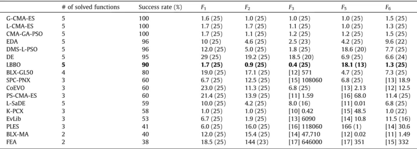
Table 1shows the results of the EAs on the 10-dimensional unimodal problems. The ‘‘# of solved functions’’ column shows how many of the benchmark problems the algorithm solved at least once out of 25 Monte Carlo simulations. The ‘‘suc-cess rate’’ column shows the percentage of simulations that suc‘‘suc-cessfully solved a problem, out of a total of (255) simulations.

Each cell inTable 1corresponds to a given algorithm and a given benchmark function, and contains two numbers whose meaning depends on whether or not the algorithm successfully solved the benchmark.

If the algorithm was successful in solving the problem at least once out of 25 simulations, then the number of successes is in round parentheses. The number outside of the parentheses is the average number of function evaluations required to achieve success divided by the success rate for that benchmark, normalized to the best CEC 2005 algorithm. For example,

Table 1

Comparison between LBBO and other EAs on five 10-dimensional unimodal problems. The algorithms are listed in order from best to worst. See the text for a more detailed description of this table. LBBO performance is shown in bold font.

# of solved functions Success rate (%) F1 F2 F3 F5 F6

G-CMA-ES 5 100 1.6 (25) 1.0 (25) 1.0 (25) 1.0 (25) 1.5 (25) L-CMA-ES 5 100 1.7 (25) 1.7 (25) 1.1 (25) 1.0 (25) 1.3 (25) CMA-GA-PSO 5 100 1.7 (25) 1.1 (25) 1.2 (25) 1.2 (25) 1.5 (25) EDA 5 96 10 (25) 4.6 (25) 2.5 (23) 4.2 (25) 9.6 (22) DMS-L-PSO 5 96 12.0 (25) 5.0 (25) 1.8 (25) 18.6 (20) 7.7 (25) DE 5 95 29 (25) 19.2 (25) 18.5 (20) 6.9 (25) 6.6 (24) LBBO 5 90 1.7 (25) 0.9 (25) 0.4 (25) 18.1 (13) 1.3 (25) BLX-GL50 4 80 19.0 (25) 17.1 (25) [12] 571 4.7 (25) 7.3 (25) SPC-PNX 3 60 6.7 (25) 12.5 (25) [15] 108060 6.8 (25) [13] 18.9 CoEVO 3 60 23.0 (25) 11.3 (25) 6.8 (25) [13] 2.13 [12] 12.5 PS-CMA-ES 3 60 21.4 (25) 13.9 (25) [11] 1.59 [16] 68.0 11.4 (25) L-SaDE 5 59 10.0 (25) 4.2 (25) 8.0 (16) [11] 0.01 6.8 (25) K-PCX 3 58 1.0 (25) 1.0 (25) [10] 0.42 [15] 48.5 1.0 (22) EvLib 3 53 6.7 (25) 1.9 (25) [13] 6090 [14] 10.8 11.5 (16) PLES 3 41 6.0 (25) 16.0 (25) [16] 118060 166 (1) [14] 30.6 BLX-MA 2 40 12.0 (25) 15.4 (25) [14] 47,710 [12] 0.02 [11] 1.49 FEA 2 38 18.5 (25) 144 (23) [17] 646000 [17] 351 [15] 332

considerF6. K-PCX was the best performing algorithm forF6. It solvedF622 out of 25 times, with an average of 7053

func-tion evaluafunc-tions in those 22 successful runs. On the other hand, LBBO solvedF625 times, with an average of 10,499

func-tion evaluafunc-tions. Therefore, the number outside of the parentheses in the LBBOF6cell inTable 1is

10499=ð25=25Þ 7053=ð22=25Þ ¼1:3

Note that these values are less than 1 for LBBO functionsF2andF3because LBBO performed better than the best 2005 CEC

algorithm for those functions.

If the algorithm wasnotsuccessful even once in solving the benchmark, then the number in square brackets indicates the performance rank of the algorithm for that particular problem, out of all the algorithms listed in the table. In this case, the number outside of the square brackets shows the normalized function value that was achieved by the algorithm, averaged over 25 Monte Carlo simulations.

Table 1shows that LBBO is able to solve all five of the unimodal benchmarks; however, six other algorithms are also able to solve all of the unimodal benchmarks, and all six of them perform better, on average, than LBBO. On the other hand, LBBO is the best algorithm for theF2andF3benchmarks.

Table 2shows the results of the EAs on the solved multimodal problems. LBBO ranks 7th best out of the 17 algorithms. LBBO is the best algorithm for theF9benchmark.

Table 3shows the results of the EAs on the most difficult 2005 CEC benchmarks: unsolved multimodal problems. LBBO ranks 5th best out of the 19 algorithms. LBBO is the best algorithm for theF8benchmark (tied with six other algorithms), and

it is also the best algorithm for theF25benchmark.

4.2.1. Summary of 10-dimensional benchmark results

Tables 1–3show that for the 10-dimensional benchmarks, LBBO ranks 7th best on the unimodal problems, 7th best on the solved multimodal problems, and 5th best on the unsolved problems. Combining the ranks of the algorithms that appear in all three of these tables, we see that overall, LBBO ranks 4th best out of the 16 algorithms.

4.3. 30-Dimensional results for the 2005 CEC benchmarks

Table 4shows results for the 30-dimensional unimodal problems for all of the EAs for which we have results. For a more detailed discussion of the meaning of the data in the table, see the beginning of Section4.2. LBBO ranks 4th best out of 13 algorithms on the unimodal benchmarks. LBBO is able to solve all five of the unimodal benchmarks. Also, LBBO is the best algorithm for theF1,F2,F3, andF6benchmarks.

Table 5shows the results of the EAs on the solved 30-dimensional multimodal problems for all of the EAs for which we have results. LBBO ranks 3rd out of the 12 algorithms. LBBO is the best algorithm for theF9,F12, andF15benchmarks.

Table 6shows the results of the EAs on the 12 unsolved 30-dimensional multimodal problems for all of the EAs for which we have results. LBBO ranks 12th out of the 15 algorithms.

Table 2

Comparison between LBBO and other EAs on six solved 10-dimensional multimodal problems. The algorithms are listed in order from best to worst. See the text for a more detailed description of this table. LBBO performance is shown in bold font.

# of solved functions Success rate (%) F7 F9 F10 F11 F12 F15

CMA-GA-PSO 6 96 1.0 (25) 2.6 (25) 1.1 (24) 0.1 (25) 2.1 (25) 2.8 (20) PS-CMA-ES 6 75 5.1 (25) 0.4 (25) 0.2 (25) 0.4 (10) 3.4 (25) 27.2 (2) G-CMA-ES 5 63 1.0 (25) 4.5 (19) 1.2 (23) 1.4 (6) 4.0 (22) [10] 28.0 DE 5 30 255 (2) 10.6 (11) [16] 36.0 1.0 (12) 8.8 (19) 75.8 (1) L-SaDE 4 53 36.2 (6) 1.0 (25) [6] 5.0 [11] 4.9 3.9 (25) 1.0 (23) DMS-L-PSO 4 47 126 (4) 2.1 (25) [5] 3.6 [10] 4.6 6.6 (19) 1.7 (22) LBBO 4 45 17.4 (20) 0.2 (25) [11] 14.4 [13] 6.1 6.5 (23) 1.0 (17) K-PCX 3 40 [14] 0.23 2.9 (24) 1.0 (22) [14] 6.7 1.0 (14) [17] 510 EvLib 3 33 [17] 1270 0.1 (25) [12] 18.6 [12] 5.2 35.3 (5) 1.7 (19) BLX-GL50 3 17 12.3 (9) 10.0 (3) [6] 5.0 [7] 2.3 12.1 (13) [16] 400 EDA 3 9 404 (1) [14] 5.4 [8] 5.3 2.9 (3) 4.3 (10) [14] 365 FEA 2 28 [15] 1.84 0.5 (25) [13] 23.4 [15] 7.0 [16] 271 0.4 (17) L-CMA-ES 2 25 1.2 (25) [17] 44.9 [17] 40.8 [8] 3.7 11.6 (12) [11] 211 BLX-MA 2 15 [13] 0.20 5.7 (18) [9] 5.6 [9] 4.6 [14] 74.3 8.5 (5) SPC-PNX 2 1 383 (1) [13] 4.0 [10] 7.3 5.8 (1) [15] 260 [12] 254 PLES 1 1 [16] 4.09 [15] 16.7 [14] 25.6 [17] 9.5 182 (1) [15] 380 CoEVO 0 0 [12] 0.037 [16] 19.2 [15] 26.8 [16] 9.0 [17] 605 [13] 294

4.3.1. Summary of 30-dimensional benchmark results

Tables 4–6show that for the 30-dimensional benchmarks, LBBO ranks 4th best on the unimodal problems, 3rd best on the solved multimodal problems, and 12th best on the unsolved problems. Combining the ranks of the algorithms that appear in all three of these tables, we see that overall, LBBO ranks 4th best out of the 11 algorithms.

Table 3

Comparison between LBBO and other EAs on 12 unsolved 10-dimensional multimodal problems. The algorithms are listed in order from best to worst. See the text for a more detailed description of this table. LBBO performance is shown in bold font.

Ave. rankF8 F13 F14 F16 F18 F19 F20 F21 F22 F23 F24 F25 G-CMA-ES 4.3 [1] 20.0 [11] 0.70 [11] 3.01 [4] 91 [2] 332 [3] 326 [1] 300 [4] 500 [6] 729 [1] 559 [1] 200 [6] 374 IPOP-CMA-ES 4.3 [9] 20.2 [12] 0.71 [1] 2.03 [2] 89 [3] 360 [2] 320 [3] 340 [4] 500 [5] 728 [1] 559 [1] 200 [9] 403 L-SaDE 6.8 [1] 20.0 [2] 0.22 [10] 2.92 [8] 101 [11] 719 [11] 705 [11] 713 [2] 464 [8] 735 [9] 664 [1] 200 [7] 376 DMS-L-PSO 7.8 [1] 20.0 [4] 0.37 [5] 2.36 [6] 95 [13] 761 [12] 714 [16] 822 [8] 536 [4] 692 [11] 730 [10] 224 [4] 366 LBBO 8.0 [1] 20.0 [5] 0.40 [14] 3.51 [13] 134 [10] 511 [7] 516 [8] 538 [7] 506 [11] 748 [10] 712 [9] 220 [1] 216 PS-CMA-ES 8.0 [12] 20.3 [5] 0.40 [13] 3.47 [3] 90 [6] 472 [6] 467 [7] 494 [9] 557 [1] 587 [8] 643 [17] 403 [9] 403 BLX-GL50 8.1 [15] 20.4 [13] 0.75 [3] 2.17 [5] 94 [4] 420 [5] 449 [6] 446 [14] 689 [14] 759 [6] 639 [1] 200 [11] 404 DE 8.2 [15] 20.4 [17] 1.81 [15] 3.52 [18] 173 [1] 300 [1] 300 [1] 300 [4] 500 [7] 734 [1] 559 [1] 200 [17] 928 EvLib 8.8 [1] 20.0 1 (10) [7] 2.81 [16] 157 [9] 500 [10] 666 [9] 585 [11] 638 [17] 792 [5] 600 [1] 200 [18] 1757 EDA 8.9 [12] 20.3 [18] 1.84 [6] 2.63 [14] 144 [7] 483 [9] 564 [10] 652 [3] 484 [15] 771 [7] 641 [1] 200 [5] 373 SPC-PNX 9.4 [19] 21.0 [15] 0.84 [12] 3.05 [12] 110 [5] 440 [4] 380 [4] 440 [13] 680 [12] 749 [4] 576 [1] 200 [12] 406 L-CMA-ES 9.5 [1] 20.0 [8] 0.49 [18] 4.01 [11] 105 [8] 497 [7] 516 [5] 442 [1] 404 [9] 740 [12]791 [19] 865 [15] 442 BLX-MA 10.8 [9] 20.2 [14] 0.77 [1] 2.03 [10] 102 [16] 803 [15] 763 [14] 800 [15] 722 [3] 671 [15] 927 [10] 224 [8] 396 K-PCX 10.8 [1] 20.0 [10] 0.65 [4] 2.35 [7] 96 [12] 752 [14] 751 [15] 813 [18] 1050 [2] 659 [17] 1060 [18] 406 [12] 406 STS 11.0 [9] 20.2 [7] 0.45 [9] 2.87 [8] 101 [14] 772 [13] 730 [12] 716 [12] 656 [13] 758 [14] 864 [10] 224 N/A RMA 12.1 [15] 20.4 [9] 0.63 [8] 2.84 [1] 84 [15] 779 [15] 763 [13] 751 [16] 747 [10] 742 [16] 931 [13] 236 [14] 410 FEA 14.1 [8] 20.1 [3] 0.32 [16] 3.53 [17] 158 [18] 909 [18] 900 [18] 951 [17] 1020 [18] 846 [19] 1130 [15] 289 [2] 256 CoEVO 14.4 [12] 20.3 [16] 1.14 [17] 3.71 [19] 177 [17] 902 [17] 845 [17] 863 [10] 635 [16] 779 [13] 835 [16] 314 [3] 257 PLES 17.6 [15] 20.4 [19] 8.7 [19] 4.14 [15] 147 [19] 1015 [19] 1002 [19] 999 [19] 1079 [19] 880 [18] 1114 [14] 282 [16] 692 Table 4

Comparison between LBBO and other EAs on five 30-dimensional unimodal problems. The algorithms are listed in order from best to worst. See the text for a more detailed description of this table. LBBO performance is shown in bold font.

# of solved functions Success rate (%) F1 F2 F3 F5 F6

G-CMA-ES 5 100 1.7 (25) 1.1 (25) 1 (25) 1 (25) 1 (25) L-CMA-ES 5 100 1.8 (25) 1.2 (25) 1 (25) 1.1 (25) 1.1 (25) CMA-GA-PSO 5 99 1.7 (25) 1.2 (25) 1.2 (25) 1.5 (24) 3.3 (25) LBBO 5 83 0.99 (25) 0.4 (25) 0.2 (25) [4] 1.7 0.8 (25) DMS-L-PSO 4 76 1.9 (25) 10.8 (25) 7.9 (21) N/A 5.5 (24) EDA 3 60 55.6 (25) 13.3 (25) 5.1 (25) [5] 0.055 [10] 21.1 BLX-GL50 3 60 21.5 (25) 13.3 (25) [9] 3112 [7] 332.6 3.7 (25) K-PCX 3 51 1 (25) 1 (25) [7] 57.9 [8] 2040 1.1 (14) DE 2 40 51.9 (25) 20.5 (25) [10] 3E5 [6] 235 [9] 3.77 SPC-PNX 3 38 11.1 (25) 26.7 (22) [12] 1E6 [10] 4237 86.7 (1) BLX-MA 1 20 11.9 (25) [12] 8E6 [11] 9E5 [9] 2183 [11] 49.5 CoEVO 2 9 519 (3) 70.0 (8) [8] 367 [11] 8344 [13] 1211 FEA 0 0 [13] 70.6 [13] 982 [13] 7E6 [12] 9913 [12] 258 Table 5

Comparison between LBBO and other EAs on six solved 30-dimensional multimodal problems. The algorithms are listed in order from best to worst. See the text for a more detailed description of this table. LBBO performance is shown in bold font.

# of solved functions Success rate F7 F9 F10 F11 F12 F15

CMA-GA-PSO 6 52 1.3 (25) 3.7 (23) 7.6 (3) 0.03 (22) 6.7 (2) 1.0 (3) G-CMA-ES 5 31 1.0 (25) 8.0 (9) 5.3 (3) 1.0 (1) 1.3 (8) [4] 208 LBBO 4 38 12.4 (24) 0.15 (25) [8] 172 [6] 28.1 0.5 (5) 1.0 (3) DE 2 31 32.8 (22) 0.7 (25) [6] 61.6 [10] 32.6 [7] 8430 [11] 484 K-PCX 4 31 2.5 (10) 3.3 (18) 1.0 (14) [7] 29.5 1.0 (5) [12] 876 EDA 1 17 21.3 (25) [11] 179 [10] 189 [12] 39.5 [6] 6054 [9] 396 L-CMA-ES 1 17 1.1 (25) [12] 291 [12] 563 [3] 15.2 [10] 13,200 [3] 21.6 BLX-GL50 1 17 10.2 (25) [7] 15.1 [4] 35.2 [5] 24.7 [8] 9521 [5] 304 SPC-PNX 1 11 60.7 (16) [8] 23.9 [5] 60.3 [4] 18.1 [9] 13,134 [8] 368 CoEVO 1 7 93.4 (11) [10] 131 [11] 232 [11] 37.7 [12] 1E5 [10] 411 BLX-MA 1 6 [11] 0.01 6.7 (9) [7] 90.6 [8] 31.1 [5] 4391 [7] 356 FEA 0 0 [12] 3.6 [9] 24.1 [9] 186 [9] 31.4 [11] 14,819 [6] 341

4.4. Discussion of the 2005 CEC benchmark results

The results of the previous sections reveal some interesting characteristics of LBBO.

In general, LBBO performs well on unimodal benchmarks. It ranks 7th out of 17 algorithms for the 10-dimensional prob-lems, and it ranks 4th out of 13 for the 30-dimensional problems. In addition, it obtained the best performance on two of the five problems in 10 dimensions, and on four of the five problems in 30 dimensions.

LBBO performs well for multimodal benchmarks with known solutions. LBBO ranks 7th out of 17 algorithms for the 10-dimensional problems, and 3rd out of 12 algorithms for the 30-10-dimensional problems. This implies that LBBO is suitable for multimodal problems that are not too difficult.

LBBO’s performance was mediocre for high-dimensional unsolved multimodal problems. LBBO ranks 5th out of 19 algo-rithms for the 10-dimensional problems, but only 12th out of 15 algoalgo-rithms for the 30-dimensional problems. This implies that LBBO may not be the best choice for extremely difficult, high-dimensional, multimodal problems. However, we will see in the following section that this does not imply that LBBO is unsuitable for real-world problems. The unsolved multimodal problems may be artificially difficult, and may therefore not be a good indication of real-world performance.

Next we compare LBBO performance onF9withF10(a rotated version ofF9), andF15withF16(a rotated version ofF15).

LBBO ranks first on the non-rotated functionsF9andF15in both 10 dimensions and 30 dimensions. However, LBBO ranks

much worse on the rotated functionsF10andF16. Superficially, this may lead one to conclude that LBBO does not perform

well on rotated functions. However, a rotated function may be quite different than its original version, and so the com-parison of performances may not be meaningful. For example, the solution of the 10-dimensional Rastrigin benchmarkF9

is within the search space, but the solution of the rotated versionF10is outside the search space. Also, since we obtainF10

by rotatingF9with rotation matrixM, that means we obtainF9by rotatingF10with rotation matrixM1. Therefore, in

general, it is not meaningful to say that an optimization algorithm performs well, or poorly, on rotated functions. There are exactly the same number of functions for which rotation deteriorates the performance of an algorithm, as there are functions for which rotation improves the performance. Note that this is not the same as saying that an algorithm is rota-tionally invariant – otherwise all algorithms would be rotarota-tionally invariant. Many benchmarks are separable under a specific rotation, and certain algorithms perform well only on separable functions. Those algorithms will thus perform well only if the benchmark is rotated with a specific rotation matrix. Rotational invariance means that an algorithm per-forms equally well on separable and nonseparable functions.

LBBO performs just as well on functions whose solution lies on the search domain boundary, as on functions whose solu-tion lies within the boundary.F20is a version ofF18with the global optimum on the domain boundary. In both 10 and 30

dimensions, LBBO performed slightly better onF20than it did onF18. LBBO’s slightly better performance onF20may be due

to the boundary search logic described in Section3.3.

LBBO performs just as well on functions with narrow optimum basins as on functions with wider basins.F19is a version of

F18with a narrow global optimum basin. LBBO performed relatively better onF19than onF18in 10 dimensions, and its

performance was the same onF19andF18in 30 dimensions. LBBO’s slightly better performance onF19may be due to

the local gradient search logic described in Section3.2.

LBBO performs just as well on functions whose optimum is outside the initialization domain, as on functions whose opti-mum is within the initialization range.F25is a version ofF24with its optimum outside the initialization range. In both 10

and 30 dimensions, LBBO performed about the same onF25as onF24. In fact, its equivalent performance onF25andF24

resulted in its being ranked 1st onF25in 10 dimensions. This may be due to several factors. First, the migration logic

Table 6

Comparison between LBBO and other EAs on 12 unsolved 30-dimensional multimodal problems. The algorithms are listed in order from best to worst. See the text for a more detailed description of this table. LBBO performance is shown in bold font.

Ave. rankF8 F13 F14 F16 F18 F19 F20 F21 F22 F23 F24 F25 ADE 1.7 [1] 20.0 [1] 1.11 [4] 12.5 [3] 52.3 [1] 716 [1] 806 [1] 619 [2] 500 [1] 500 [1] 534 [1] 200 [3] 210 IPOP-CMA-ES 4.1 [9] 20.8 [7] 2.53 [1] 11.0 [1] 11.1 [8] 904 [8] 904 [7] 904 [2] 500 [3] 817 [1] 534 [1] 200 [1] 209 G-CMA-ES 5.3 [5] 20.1 [5] 2.49 [7] 12.9 [2] 35.0 [8] 904 [8] 904 [7] 904 [2] 500 [2] 803 [1] 534 [13] 910 [4] 211 RMA 5.3 [10] 20.9 [6] 2.50 [5] 12.6 [7] 85.7 [7] 902 [5] 902 [11] 906 [2] 500 [4] 867 [1] 534 [1] 200 [4] 211 EDA 5.6 [10] 20.9 [15]15.3 [12] 13.3 [10] 208 [3] 847 [3] 842 [3] 851 [2] 500 [6] 872 [1] 534 [1] 200 [1] 209 BLX-MA 6.3 [8] 20.7 [9] 3.96 [5] 12.6 [14] 326 [4] 878 [4] 880 [4] 879 [2] 500 [9] 908 [8] 559 [1] 200 [7] 212 STS 6.4 [7] 20.5 [2] 1.72 [2] 11.8 [9] 121 [6] 891 [5] 902 [6] 897 [2] 500 [11] 991 [9] 575 [11] 445 N/A L-CMA-ES 6.8 [1] 20.0 [4] 2.32 [15] 14.0 [4] 58.4 [5] 890 [7] 903 [5] 889 [1] 485 [5] 871 [7] 535 [15] 1410 [12] 691 SPC-PNX 7.2 [10] 20.9 [8] 3.59 [10] 13.1 [6] 74.0 [11] 905 [11] 905 [10] 905 [2] 500 [8] 880 [1] 534 [1] 200 [8] 213 BLX-GL50 8.0 [15] 21.0 [11] 5.15 [3] 12.1 [8] 88.7 [8] 904 [8] 904 [7] 904 [2] 500 [7] 874 [11] 587 [12] 877 [4] 211 K-PCX 8.2 [1] 20.0 [14] 11.9 [14] 13.8 [5] 71.5 [2] 830 [2] 831 [2] 831 [15] 859 [15] 1560 [13] 866 [7] 213 [8] 213 LBBO 8.8 [1] 20.0 [3] 2.26 [9] 13.1 [12] 273 [13] 933 [13] 930 [13] 929 [2] 500 [12] 1073 [10] 582 [8] 264 [10] 270 DE 11.4 [10] 20.9 [10] 4.51 [12] 13.3 [13] 282 [12] 913 [12] 913 [12] 913 [12] 581 [10] 964 [12] 621 [9] 314 [13] 786 FEA 11.8 [6] 20.3 [12] 5.57 [8] 12.9 [11] 270 [14] 964 [14] 943 [14] 967 [14] 695 [13] 1080 [14] 910 [10] 328 [11] 517 CoEVO 13.7 [10] 20.9 [13] 9.02 [11] 13.2 [15] 381 [15] 1061 [15] 1049 [15] 1059 [13] 604 [14] 1155 [15] 922 [14] 1097 [14] 1027

of Eq.(4)allows an LBBO offspring variable to move outside of the range of its parents. Second, the mutation described in Section2.2, and the Latin hypercube search and re-initialization described in Sections3.5 and 3.6, are allowed to search outside the initialization boundaries if the optimum is known a priori to lie outside those boundaries.

The inclusion of seven new components to BBO to obtain the LBBO procedure ofAlgorithm 8improves performance, but results in a higher computational cost. The increased computational cost varies depending on the particular random num-ber sequence realization for a particular simulation, and depending on the cost function. However, the vast majority of computational effort in interesting, real-world problems is consumed with fitness function evaluations, and so the com-putational effort of the optimization algorithm is rarely significant as discussed in Section 21.1 of[63]. This consideration leads us to study LBBO performance on real-world benchmarks in the following section.

4.5. 2011 CEC benchmarks

Next we test the performance of the proposed LBBO method on the 22 real-world benchmark functions from the 2011 CEC. These problems include a parameter estimation problem for frequency-modulated sound saves (T1); a Lennard-Jones

potential problem (T2); a bifunctional catalyst blend control problem (T3); a stirred tank reactor control problem (T4); two

Tersoff potential minimization problems (T5andT6); a radar polyphase code design problem (T7); a transmission network

expansion problem (T8); a transmission pricing problem (T9); an antenna array design problem (T10); two dynamic economic

dispatch problems (T11.1andT11.2); five static economic dispatch problems (T11.3T11.7); three hydrothermal scheduling

problems (T11.8T11.10); and two spacecraft trajectory optimization problems (T12andT13). The dimensions of these

prob-lems range from a minimum of 1 to a maximum of 216. The benchmarks include unconstrained probprob-lems, equality-con-strained problems, and inequality conequality-con-strained problems. Constraints are augmented to the cost functions as penalty terms. For details about these functions, the reader is referred to[14,56]. As in the 2011 CEC, in this paper we limit each simulation to 150,000 function evaluations. LBBO parameters are the same as those described at the beginning of Section4.1.

We compared LBBO algorithms to the 14 algorithms that were accepted for the 2011CEC competition. 1. GAMPC, which is a GA with multi-parent crossover[18].

2. SAMODE, which is differential evolution with a mixture of search operators[19]. 3. ENSDE, which is ensemble-based differential evolution[41].

4. EADEMA, which is a hybrid of a memetic algorithm and a differential evolution variant[58]. 5. AdapDE, which is adaptive differential evolution[3].

6. EDDE, which is a hybrid of estimation of distribution and differential evolution[71]. 7. OXDE, which is differential evolution with orthogonal crossover[33].

8. DERHC, which is a hybrid of differential evolution and random hill climbing[31]. 9. RGA, which is a real-coded GA[55].

10. CDASA, which is an ant system[28].

11. mSBXGA, which is a GA with simulated binary crossover[7].

12. DEcr, which is differential evolution with adaptive crossover and local search[52]. 13. WIDE, which is a hybrid of invasive weed optimization and differential evolution[24]. 14. ModDELS, which is differential evolution with local search[2].

We collected benchmark performance data for these EAs from[67,68]. As in the 2011 CEC competition, we ran 25 Monte Carlo simulations of LBBO for each benchmark, and then ranked all of the algorithms based on both the best cost achieved out of 25 simulations, and the average cost achieved over 25 simulations.Tables 7 and 8show the results. Note that the rank-ings in these tables differ slightly from those reported in[68]. This is because we used all reported significant digits in deter-mining the rankings reported in this paper, whereas[68]rounded the results to a given number of significant digits for each benchmark.Table 7shows that in terms of the best cost achieved, LBBO performs third best out of 15 algorithms.Table 8 shows that in terms of the average cost achieved, LBBO performs fourth best.

Tables 7 and 8show that LBBO performs relatively poorly on benchmarksT1,T10,T11.9, andT11.10. LBBO’s poor

perfor-mance onT1could simply be a matter of reporting precision. The best seven algorithms reported a best cost of exactly 0

forT1, while LBBO reported a best cost of 1.831015. So although it appears fromTables 7 and 8that LBBO has poor

per-formance onT1, its performance may be the best for all practical purposes. We see a similar phenomenon withT10. However,

LBBO’s poor performance onT11.9andT11.10is more difficult to explain. LBBO clearly performs poorly on these two

bench-marks, with average costs of 2.2106_{and 1.8}

106_{respectively, compared to average costs by the best algorithm (DEcr) of}

9.3105_{and 9.2}

105_{respectively.T}

11.9andT11.10are hydrothermal scheduling problems, but so isT11.8, for which LBBO

attained the best ranking.

Tables 7 and 8shows that LBBO performs exceptionally well on benchmarksT11.1,T11.2,T11.5,T11.6,T11.7, andT11.8, where

LBBO’s performance ranks at the top in terms of both the best cost attained and the average cost attained. In general, these six benchmarks have the common feature of high dimensionality, with problem dimensions of 120, 216, 15, 40, 140, and 96 respectively. These problems include the ones with the highest, third highest, fourth highest, and fifth highest dimensions. Also, LBBO performs third best (on average) on the problem with the second highest dimension (T9). So in general, LBBO

Another common feature of the benchmarks for which LBBO performs well is inequality constraints. The 2011 CEC bench-marks augment inequality constraints to the original cost function with a penalty function. This results in augmented cost functions with deep, narrow valleys at their constrained minima. Of the 22 benchmarks, 10 of them have only inequality constraints (no equality constraints), and all six of the benchmarks for which LBBO performs best belong to that group.

In summary, we conclude that, in general, LBBO performs particularly well on high-dimensional problems with the type of deep, narrow optima that characterizes cost functions that are augmented with inequality constraints.

5. The relative importance of LBBO components

Section3shows that LBBO includes seven components that are added to BBO: migration (Section3.1), gradient descent (Section3.2), boundary search (Section3.3), grid search (Section3.4), Latin hypercube search (Section3.5), re-initialization (Section3.6), and restart (Section3.7). The issue that we address in this section is the relative importance of each of these components.

First we run LBBO with all seven components except the first one; that is, we replace the unique LBBO migration logic of Section3.1with the standard BBO migration logic of Section2.1. Next, we run LBBO with all seven components except the second one; that is, we skip the gradient descent logic of Section3.2. In general, we run LBBO with all seven components except thenth one, forn

e

[1, 7].

We repeat the 10-dimensional benchmark tests of Section4.2under these conditions. Results for the unimodal problems, the solved multimodal problems, and the unsolved multimodal problems are shown inTables 9–11respectively.

Table 12shows the results of pair-wise Wilcoxon signed rank tests[45]between the complete LBBO algorithm with all seven additional components, and each algorithm that has a single component removed. Each cell inTable 12indicates whether the given algorithm with a single component removed performs better than, worse than, or statistically equal to the complete LBBO algorithm on the given benchmark, where we used 95% as the confidence threshold.

Table 7

Comparison between LBBO and 14 other EAs on real-world benchmark problems in terms of the best results obtained after 25 Monte Carlo simulations. The table shows the rank of each algorithm, and the algorithms are listed in order from best to worst. This table shows the ranks of the algorithms in terms of best results, whileTable 8shows the ranks in terms of average results. LBBO performance is shown in bold font.

T1 T2 T3 T4 T5 T6 T7 T8 T9 T10 T11.1 T11.2 T11.3 T11.4 T11.5 T11.6 T11.7 T11.8 T11.9 T11.10 T12 T13 Ave. GAMPC 1 4 1 3 7 2 1 1 5 3 4 4 1 2 3 5 11 10 4 7 3 1 3.8 DEcr 11 4 1 3 7 1 9 1 13 10 2 2 1 1 3 2 2 2 1 1 10 9 4.4 LBBO 10 4 1 3 2 2 8 1 4 10 1 1 1 6 1 1 1 1 14 14 5 8 4.5 SAMODE 1 4 1 3 7 2 1 1 9 3 7 4 1 9 9 6 11 9 7 8 2 2 4.9 OXDE 1 1 1 1 6 14 1 1 13 1 10 4 1 2 3 6 4 7 8 12 6 5 4.9 EDDE 1 4 1 3 2 2 7 1 15 3 7 4 1 6 9 6 6 4 6 3 8 13 5.1 WIDE 1 4 14 3 7 2 1 1 10 3 7 4 1 2 3 9 7 11 5 9 1 7 5.1 AdapDE 1 2 13 14 5 10 1 1 1 2 3 9 10 8 7 3 5 3 2 2 11 3 5.3 ENSDE 1 15 1 3 15 15 15 1 7 3 5 3 1 2 2 4 7 4 3 3 14 6 5.9 RGA 15 11 1 3 7 2 11 1 3 13 12 13 14 10 9 14 7 6 10 5 7 10 8.4 CDASA 9 13 1 3 7 2 10 1 6 15 6 11 14 12 14 11 3 7 9 5 13 14 8.5 EADEMA 12 3 1 12 1 11 1 1 2 8 15 15 11 11 8 15 14 15 12 15 4 4 8.7 DERHC 8 4 1 15 2 2 14 1 8 14 11 14 1 12 15 13 15 14 15 13 15 15 10.1 mSBXGA 14 12 12 13 13 12 12 1 11 12 14 10 13 14 9 10 10 12 11 10 12 12 11.3 ModDELS 13 14 14 2 14 13 13 1 12 9 13 12 12 15 13 12 13 13 13 11 9 11 11.5 Table 8

Comparison between LBBO and 14 other EAs on real-world benchmark problems in terms of the average results obtained by 25 Monte Carlo simulations. The table shows the rank of each algorithm, and the algorithms are listed in order from best to worst. This table shows the ranks of the algorithms in terms of average results, whileTable 7shows the ranks in terms of best results. LBBO performance is shown in bold font.

T1 T2 T3 T4 T5 T6 T7 T8 T9 T10 T11.1 T11.2 T11.3 T11.4 T11.5 T11.6 T11.7 T11.8 T11.9 T11.10 T12 T13 Ave. GAMPC 1 2 1 1 5 5 5 1 6 1 4 3 1 4 3 5 7 10 4 8 2 1 3.6 DEcr 4 2 1 13 6 1 9 1 14 13 2 2 1 1 3 2 2 2 1 1 10 7 4.5 SAMODE 5 4 1 5 12 4 7 1 8 1 7 3 1 7 3 5 9 8 7 7 1 2 4.9 LBBO 10 1 1 1 1 7 6 1 3 9 1 1 10 7 1 1 1 1 14 15 6 14 5.1 EDDE 1 9 1 1 11 7 14 1 15 5 4 7 1 4 8 5 3 4 5 3 7 9 5.7 OXDE 12 5 1 11 9 14 4 1 13 4 8 3 1 4 3 8 4 6 8 13 4 6 6.5 AdapDE 9 6 1 14 10 11 1 1 1 8 12 9 10 9 8 3 6 3 3 2 14 3 6.5 WIDE 8 11 14 8 4 10 3 1 10 1 11 7 1 3 3 10 12 12 6 11 9 4 7.2 ENSDE 6 14 1 12 14 15 15 1 9 14 6 3 10 1 2 4 4 5 2 4 12 5 7.2 RGA 14 12 1 5 7 3 11 1 2 12 9 13 10 11 8 14 14 9 10 6 8 8 8.5 ModDELS 3 13 14 1 8 11 8 1 12 7 13 12 7 12 13 11 7 11 13 9 3 11 9.1 EADEMA 7 10 1 9 2 6 2 1 4 6 15 15 8 14 12 15 15 15 15 14 5 12 9.2 DERHC 13 7 1 15 3 2 13 1 7 11 9 14 10 13 14 12 12 13 11 10 13 13 9.9 CDASA 15 15 1 5 15 9 10 1 5 15 3 11 10 15 15 13 11 6 9 5 15 15 10.0 mSBXGA 11 8 13 10 13 13 12 1 11 10 14 10 9 10 8 9 10 14 12 12 11 10 10.5

Tables 9–12show that the worst-performing algorithm is LBBO without gradient descent, which performs worse than LBBO on 20 of the 23 benchmarks. This means that gradient descent is the most important feature of our LBBO algorithm. We conclude that LBBO is not very effective unless it is augmented with a local search method such as gradient descent.

Tables 9–12also show that some of the algorithms perform better than LBBO on certain benchmarks. This is most clear fromTable 12, where we see that LBBO without grid search performs better than LBBO on five benchmarks, although LBBO still performs better on seven benchmarks.

In general, we conclude that gradient descent is the most important feature of LBBO, and grid search is the least important feature. For the simplest functions like the unimodal functions ofTable 9, all of the features are of secondary importance compared to gradient descent. For solved multimodal functions (Table 10), the restart and grid search features are also important, but still less important than gradient descent. For the most difficult problems (the unsolved multimodal functions ofTable 11), all of the LBBO features appear to be important except Latin hypercube search and periodic re-initialization.

The only gradient descent algorithm that we tested was the interior point algorithm as implemented by MATLAB’s fmin-confunction. We have not implemented our own local optimization algorithm, or tested other algorithms as alternatives to

fmincon, but that could be an important task for future research. How important is the particular gradient descent algorithm that we used? The gradient descent algorithm, along with its settings, can be considered to be tuning parameters of LBBO. This section has shown the relative importance of each component of LBBO by eliminating one component at a time. It would also be interesting to study this question from the opposite perspective; that is, start with standard BBO and add one component at a time to see how each component affects performance in isolation from the other components. Such a study may give different results than what we conclude here, and we suggest that idea for future research.

Table 9

Comparison between LBBO, and LBBO with thenth component omitted forne[1, 7], on 10-dimensional unimodal problems. The algorithms are listed in order from best to worst. See Sections4.2 and 5for a more detailed description of this table. Note that the last seven rows of the table show the performance of the complete LBBO algorithm except for the omission of a single algorithmic component.

# of solved functions Success rate (%) F1 F2 F3 F5 F6

LBBO 5 90 1.7 (25) 0.9 (25) 0.4 (25) 18.1 (13) 1.5 (25) No grid search 5 88 1.7 (25) 0.8 (25) 0.3 (25) 23.9 (10) 1.2 (25) Std. migration 5 84 3.5 (25) 1.9 (25) 0.8 (25) 19.5 (5) 1.6 (25) No Latin 5 84 3.5 (25) 1.8 (25) 0.9 (25) 51.4 (5) 1.7 (25) No restart 5 83 4.2 (25) 1.7 (25) 0.9 (25) 32.2 (4) 1.6 (25) No re-init 5 82 3.3 (25) 2.1 (25) 0.9 (25) 73.9 (3) 1.7 (25) No boundary 4 80 3.9 (25) 2.2 (25) 0.9 (25) [7] 0.59 1.5 (25) No gradient 0 0 [8] 508 [8] 2405 [8] 4.9E5 [8] 3725 [8] 5.3E6

Table 10

Comparison between LBBO, and LBBO with thenth component omitted forne[1, 7], on solved 10-dimensional multimodal problems. The algorithms are listed in order from best to worst. See Sections4.2 and 5for a more detailed description of this table. Note that the last seven rows of the table show the performance of the complete LBBO algorithm except for the omission of a single algorithmic component.

# of solved functions Success rate (%) F7 F9 F10 F11 F12 F15

LBBO 4 57 17.4 (20) 0.2 (25) [4] 14.4 [8] 6.1 6.3 (23) 1.0 (17) Std. migration 3 50 [5] 1.2 0.2 (25) [1] 11.9 [3] 5.5 3.1 (25) 0.5 (25) No boundary 3 50 [5] 1.2 0.2 (25) [2] 12.6 [6] 5.8 3.1 (25) 0.6 (25) No re-init. 3 50 [4] 1.1 0.2 (25) [6] 16.0 [5] 5.7 5.4 (25) 0.6 (25) No Latin 3 49 [3] 1.0 0.2 (25) [5] 15.4 [7] 5.9 4.2 (25) 0.8 (23) No restart 3 36 [7] 1.3 0.2 (25) [7] 17.9 [1] 5.1 6.6 (17) 0.6 (12) No grid search 2 27 14.2 (16) [7] 7.0 [3] 14.2 [2] 5.4 4.5 (25) [7] 138 No gradient 0 0 [8] 18.6 [8] 15.9 [8] 27.3 [4] 5.6 [8] 1.0E4 [8] 142 Table 11

Comparison between LBBO, and LBBO with thenth component omitted forne[1, 7], on unsolved 10-dimensional multimodal problems. The algorithms are listed in order from best to worst. See Sections4.2 and 5for a more detailed description of this table. Note that the last seven rows of the table show the performance of the complete LBBO algorithm except for the omission of a single algorithmic component.

F8 F13 F14 F16 F18 F19 F20 F21 F22 F23 F24 F25 LBBO [1] 20.0 [1] 0.40 [3] 3.51 [2] 134 [1] 511 [1] 516 [1] 538 [2] 506 [2] 748 [5] 712 [6] 220 [4] 216 No Latin [1] 20.0 [4] 0.45 [1] 3.35 [6] 139 [3] 762 [3] 766 [3] 747 [1] 491 [5] 760 [2] 598 [1] 205 [1] 205 No re-init [1] 20.0 [2] 0.41 [2] 3.41 [4] 137 [2] 754 [2] 762 [2] 744 [5] 574 [7] 797 [3] 618 [2] 206 [1] 205 Std. migration [1] 20.0 [6] 0.50 [6] 3.56 [1] 133 [5] 794 [5] 826 [6] 818 [4] 541 [6] 784 [1] 588 [4] 215 [4] 216 No boundary [1] 20.0 [7] 0.51 [8] 3.91 [5] 138 [6] 797 [4] 783 [4] 776 [3] 513 [1] 728 [4] 662 [3] 212 [3] 213 No grid search [1] 20.0 [5] 0.48 [5] 3.54 [2] 134 [4] 782 [7] 831 [4] 776 [6] 577 [3] 749 [7] 882 [5] 219 [6] 223 No restart [1] 20.0 [2] 0.41 [4] 3.52 [7] 144 [8] 902 [8] 912 [8] 906 [8] 902 [4] 756 [8] 925 [7] 296 [7] 380 No gradient [8] 20.3 [8] 0.52 [7] 3.57 [8] 167 [7] 826 [6] 827 [7] 858 [7] 819 [8] 837 [6] 746 [8] 441 [8] 488

6. Conclusions and future work

A linearized version of BBO, LBBO, was introduced in this paper. LBBO modifies the BBO migration operator to reduce rotational variance. In addition, we included global and local search operators, along with re-initialization logic, to improve performance.

LBBO was compared with the entries to the 2005 Congress on Evolutionary Computation on 23 benchmark problems. The results show that LBBO provides competitive performance. LBBO performs particularly well for certain types of multimodal problems. Also, LBBO is insensitive to whether or not the solution lies on the search domain boundary, to whether or not the global optimum lies in a wide or narrow basin, and to whether or not the global optimum lies within or outside of the ini-tialization domain. Compared to 11 other EAs, LBBO performed the best for 5 out of 23 benchmarks in 10 dimensions, and it performed the best for 9 out of 23 benchmarks in 30 dimensions. The improved relative performance of LBBO in 30 dimen-sions indicates that it may perform even better on higher dimensional problems, which we suggest for future research.

LBBO was also compared with the entries to the 2011 Congress on Evolutionary Computation on 22 real-world problems. The results show that LBBO performs particularly well for high dimensional problems, and for problems with inequality con-straints. Compared to 14 other EAs, LBBO performed third best in terms of best performance, and fourth best in terms of average performance.

Tables 9–11showed that local search is the most important new component that we added to BBO to obtain LBBO. We used gradient descent as a default local search operator, but our results indicate that it may be fruitful to experiment with other local search operators to improve LBBO performance.

One area in which LBBO fell short was its performance on extremely difficult (unsolved) multimodal problems, including highly nonseparable problems. This reveals an area where LBBO could be improved. Other future work could include testing on additional benchmark functions, testing with higher dimensions, noise handling, comparing LBBO with additional EAs, and hybridizing LBBO with other successful EAs. The MATLAB software that we used to generate the results in this paper is available athttp://www.academic.csuohio.edu/simond/bbo/linearized.

Acknowledgments

The comments of the reviewers were helpful in improving the original version of this paper. The material in this paper is based on work supported by the National Science Foundation under Grant No. 0826124.

Table 12

Statistical comparison between LBBO, and LBBO with a single component omitted. Each cell indicates whether the given algorithm is better than (B), worse than (W), or equal to () LBBO, based on a Wilcoxon signed rank test with a confidence threshold of 95%. The number at the bottom of each column is equal to the number of W cells minus the number of B cells. Note that the seven right-most columns of the table compare the performance of LBBO, with the complete LBBO algorithm except for the omission of a single algorithmic component.

Standard migration No boundary No gradient No grid No Latin No reinit. No restart

F1 W W B W F2 W W W B W W W F3 W W W B W W W F5 W W F6 W W W W W W F7 W W W W W W F8 W F9 B W W B B B F10 W B W W W F11 F12 W W F13 W W F14 W F15 W W F16 W F18 W W W W W W W F19 W W W W W W W F20 W W W W W W W F21 W W F22 W F23 B W B B W F24 B W B B F25 W W B B Net # Worse than LBBO 6 9 20 2 4 5 11

References

[1] S. Alonso, J. Jimenez, H. Carmona, B. Galvan, G. Winter, Performance of a flexible evolutionary algorithm, Technical Report, University of Las Palmas de Gran Canaria, Canary Islands, Spain, 2005. <http://www.ntu.edu.sg/home/epnsugan/index_files/CEC-05/CEC05.htm>.

[2] M. Ankush, A. Das, P. Mukherjee, S. Das, P. Suganthan, Modified differential evolution with local search algorithm for real world optimization, in: IEEE Congress on Evolutionary Computation, New Orleans, Louisiana, 2011, pp. 1565–1572.

[3] M. Asafuddoula, T. Ray, R. Sarker, An adaptive differential evolution algorithm and its performance on real world optimization problems, in: IEEE Congress on Evolutionary Computation, New Orleans, Louisiana, 2011, pp. 1057–1062.

[4] A. Auger, N. Hansen, A restart CMA evolution strategy with increasing population size, in: IEEE Congress on Evolutionary Computation, Edinburgh, United Kingdom, 2005, pp. 1769–1776.

[5] A. Auger, N. Hansen, Performance evaluation of an advanced local search evolutionary algorithm, in: IEEE Congress on Evolutionary Computation, Edinburgh, United Kingdom, 2005, pp. 1777–1784.

[6] P. Ballester, J. Stephenson, J. Carter, K. Gallagher, Real-parameter optimization performance study on the CEC-2005 benchmark with SPC-PNX, in: IEEE Congress on Evolutionary Computation, Edinburgh, United Kingdom, 2005, pp. 498–505.

[7] S. Bandaru, R. Tulshyan, K. Deb, Modified SBX and adaptive mutation for real world single objective optimization, in: IEEE Congress on Evolutionary Computation, New Orleans, Louisiana, 2011, pp. 1335–1342.

[8] W. Becker, X. Yu, J. Tu, EvLib: A Parameterless Self-Adaptive Real-Valued Optimisation Library, Technical Report, RMIT University, Melbourne, Australia, 2005. <http://www.ntu.edu.sg/home/epnsugan/index_files/CEC-05/CEC05.htm>.

[9]D. Bernstein, Optimization r us, IEEE Cont. Syst. Mag. 26 (5) (2006) 6–7.

[10]I. Boussaid, A. Chatterjee, P. Siarry, M. Ahmed-Nacer, Hybridizing biogeography-based optimization with differential evolution for optimal power allocation in wireless sensor networks, IEEE Trans. Veh. Technol. 60 (5) (2011) 2347–2353.

[11]J. Brown, M. Lomolino, Independent discovery of the equilibrium theory of island biogeography, Ecology 70 (6) (1989) 1954–1957. [12]M. Clerc, Beyond standard particle swarm optimisation, Int. J. Swarm Intell. Res. 1 (4) (2010) 46–61.

[13] L. Costa, A parameter-less evolution strategy for global optimization, in: WSEAS International Conference on Simulation, Modelling and Optimization, Lisbon, Portugal, 2006, pp. 622–627.

[14] S. Das, P. Suganthan, Problem definitions and evaluation criteria for CEC 2011 competition on testing evolutionary algorithms on real world optimization problems, Technical Report, Jadavpur University, Nanyang Technological University, 2010.

[15] M. Dorigo, Optimization, Learning and Natural Algorithms, PhD Thesis, Politecnico di Milano, Italy, 1992.

[16]A. Duarte, R. Martí, F. Glover, F. Gortazar, Hybrid scatter tabu search for unconstrained global optimization, Ann. Oper. Res. 183 (1) (2011) 95–123. [17]A. Eiben, J. Smith, Introduction to Evolutionary Computing, Springer, 2010.

[18] S. Elsayed, R. Sarker, D. Essam, GA with a new multi-parent crossover for solving IEEE-CEC2011 competition problems, in: IEEE Congress on Evolutionary Computation, New Orleans, Louisiana, 2011, pp. 1034–1040.

[19] S. Elsayed, R. Sarker, D. Essam, Differential evolution with multiple strategies for solving CEC2011 real-world numerical optimization problems, in: IEEE Congress on Evolutionary Computation, New Orleans, Louisiana, 2011, pp. 1041–1048.

[20] M. Ergezer, D. Simon, D. Du, Oppositional biogeography-based optimization, in: IEEE Conference on Systems, Man, and Cybernetics, San Antonio, Texas, 2009, pp. 1035–1040.

[21] C. García-Martínez, M. Lozano, Hybrid real-coded genetic algorithms with female and male differentiation, in: IEEE Congress on Evolutionary Computation, Edinburgh, United Kingdom, 2005, pp. 896–903.

[22]D. Goldberg, Genetic Algorithms in Search, Optimization and Machine Learning, Addison-Wesley, 1989.

[23]W. Gong, Z. Cai, C. Ling, DE/BBO: a hybrid differential evolution with biogeography-based optimization for global numerical optimization, Soft. Comput. 15 (4) (2011) 645–665.

[24] U. Haider, S. Das, D. Maity, A. Abraham, P. Dasgupta, Self adaptive cluster based and weed inspired differential evolution algorithm for real world optimization, in: IEEE Congress on Evolutionary Computation, New Orleans, Louisiana, 2011, pp. 750–756.

[25] N. Hansen, Compilation of results on the 2005 CEC benchmark function set, Technical Report, Computational Laboratory (CoLab), Institute of Computational Science, 2006.

[26]S. Islam, S. Das, S. Ghosh, S. Roy, P. Suganthan, An adaptive differential evolution algorithm with novel mutation and crossover strategies for global numerical optimization, IEEE Trans Syst, Man, Cybern Part B: Cybern 42 (2) (2012) 482–500.

[27] J. Kennedy, R. Eberhart, Particle swarm optimization, in: IEEE International Joint Conference on Neural Networks, Perth, Western Australia, 1995, pp. 1942–1948.

[28] P. Korosec, J. Silc, The continuous differential ant-stigmergy algorithm applied to real-world optimization problems, in: IEEE Congress on Evolutionary Computation, New Orleans, Louisiana, 2011, pp. 1327–1334.

[29]H. Kundra, M. Sood, Cross-country path finding using hybrid approach of PSO and BBO, Int. J. Comput. Appl. 7 (6) (2010) 15–19.

[30] B. Lacroix, D. Molina, F. Herrera, Region based memetic algorithm with LS chaining, in: World Congress on Computational Intelligence, Brisbane, Australia, 2012, pp. 1474–1479.

[31] A. LaTorre, S. Muelas, J.-M. Peña, Benchmarking a hybrid DE-RHC algorithm on real world problems, in: IEEE Congress on Evolutionary Computation, New Orleans, Louisiana, 2011, pp. 1027–1033.

[32]G. Leguizamón, C. Coello Coello, Boundary search for constrained numerical optimization problems, in: E. Mezura-Montes (Ed.), Constraint-Handling in Evolutionary Optimization, Springer, 2009, pp. 25–49.

[33] X. Li, M. Yin, Enhancing the Exploration Ability of Composite Differential Evolution through Orthogonal Crossover, 2011 (unpublished).

[34] J. Liang, P. Suganthan, Dynamic multi-swarm particle swarm optimizer with local search, in: IEEE Congress on Evolutionary Computation, Edinburgh, United Kingdom, 2005, pp. 522–528.

[35] T. Liao, M. Montes de Oca, T. Stützle, Computational results for an automatically tuned IPOP-CMA-ES on the CEC’05 benchmark set, Technical Report TR/IRIDIA/2011-022, Université Libre de Bruxelles, Brussels, Belgium, 2011.

[36] P. Lozovyy, G. Thomas, D. Simon, Biogeography-based optimization for robot controller tuning, in: B. Igelnik (Ed.), Computational Modeling and Simulation of Intellect: Current State and Future Perspectives, IGI Global, 2011, pp. 162–181.

[37]H. Ma, D. Simon, Analysis of migration models of biogeography-based optimization using Markov theory, Eng. Appl. Artif. Intell. 24 (2011) 1052–1060. [38]H. Ma, D. Simon, Blended biogeography-based optimization for constrained optimization, Eng. Appl. Artif. Intell. 24 (3) (2011) 517–525.

[39]H. Ma, D. Simon, M. Fei, Z. Xie, Variations of biogeography-based optimization and Markov analysis, Inf. Sci. 220 (2013) 492–506. [40]R. MacArthur, E. Wilson, The Theory of Island Biogeography, Princeton University Press, Princeton, New Jersey, 1967.

[41] R. Mallipeddi, P. Suganthan, Ensemble differential evolution algorithm for CEC2011 problems, in: IEEE Congress on Evolutionary Computation, New Orleans, Louisiana, 2011, pp. 1557–1564.

[42]M. Matsumoto, T. Nishimura, Mersenne twister: a 623-dimensionally equidistributed uniform pseudo-random number generator, ACM Trans. Model. Comput. Simul. 8 (1) (1998) 3–30.

[43] D. Molina, F. Herrera, M. Lozano, Adaptive local search parameters for real-coded memetic algorithms, in: IEEE Congress on Evolutionary Computation, Edinburgh, United Kingdom, 2005, pp. 888–895.

[44] C. Müller, B. Baumgartner, I. Sbalzarini, Particle swarm CMA evolution strategy for the optimization of multi-funnel landscapes, in: IEEE Congress on Evolutionary Computation, Trondheim, Norway, 2009, pp. 2685–2692.

[46] M. Ovreiu, D. Simon, Biogeography-based optimization of neuro-fuzzy system parameters for diagnosis of cardiac disease, in: Genetic and Evolutionary Computation Conference, Portland, Oregon, 2010, pp. 1235–1242.

[47]V. Panchal, P. Singh, N. Kaur, H. Kundra, Biogeography based satellite image classification, Int. J. Comput. Sci. Inf. Secur. 6 (2009) 269–274. [48] P. Pošik, Real parameter optimisation using mutation step co-evolution, in: IEEE Congress on Evolutionary Computation, Edinbur