SIGSPACE : CLASS-BASED FEATURE REPRESENTATION FOR SCALABLE AND DISTRIBUTED MACHINE LEARNING
A Thesis IN
Computer Science
Presented to the Faculty of the University of Missouri–Kansas City in partial fulfillment of
the requirements for the degree MASTER OF SCIENCE
by
SEETHA RAMA PRADYUMNA DODDALA
B.Tech., Jawaharlal Nehru Technological University, Hyderabad, Andhra Pradesh, INDIA, 2011
Kansas City, Missouri 2016
c 2016
SEETHA RAMA PRADYUMNA DODDALA ALL RIGHTS RESERVED
SIGSPACE : CLASS-BASED FEATURE REPRESENTATION FOR SCALABLE AND DISTRIBUTED MACHINE LEARNING
Seetha Rama Pradyumna Doddala, Candidate for the Master of Science Degree University of Missouri–Kansas City, 2016
ABSTRACT
In the era of big data, it is essential to explore the opportunities in discovering knowl-edge from big data. However, traditional machine learning approaches are not well fit to analyze the full value of big data. Explicitly, current research and practice of Ma-chine learning do not fully support some important features for big data analytics such as incremental learning, distributed learning, and fuzzy matching.
In this thesis, we propose a unique feature representation, named the SigSpace. It is designed for a class-level incremental learning in support to distributed learning and fuzzy matching. In SigSpace, a class-based model was built by an evaluation and ex-tension of existing machine learning models, i.e., K-means and Self-Organizing Maps (SOM). The Machine learning with SigSpace is modeled as a feature set with standard machine learning algorithms like Random Forests, Decision Tree etc., and a class model using L1 (Manhattan distance) and L2 (Euclidean distance) norms.
In order to provide supporting evidence for the effectiveness of SigSpace, we have conducted comprehensive experiments as follows: Firstly, multiple experiments were conducted to evaluate the SigSpace model in image classification using large scale im-age datasets including Caltech-101, Caltech-256, Imim-ageNet, UEC FOOD 256, MNIST with image features like Pixels, SIFT, and Local Binary Pattern. Secondly, SigSpace was evaluated in the audio classification context with imperative audio features extracted from real-time audio datasets.
The SigSpace system was implanted using a Big data analytics tool, Apache Spark(MLLib) with the capability of parallel and distributed learning and recognition. The experiments of multinomial classification were conducted with 6 to 1000 classes, space requirements in megabytes to terabytes, and learning time ranging from minutes to days. Although there has been a slight accuracy decrease (approximately 5%) in the over-all performance, SigSpace is very efficient, in terms of space as well as runtime perfor-mance for learning and recognition. Thus, the current evaluation confirms that SigSpace has a significant approach for distributed and scalable Machine learning with big data.
APPROVAL PAGE
The faculty listed below, appointed by the Dean of the School of Computing and Engi-neering, have examined a thesis titled “SigSpace : Class-based Feature Representation for Scalable and Distributed Machine Learning,” presented by Seetha Rama Pradyumna Dod-dala, candidate for the Master of Science degree, and hereby certify that in their opinion it is worthy of acceptance.
Supervisory Committee
Dr. Yugyung Lee, Ph.D., Committee Chair
Department of Computer Science & Electrical Engineering Dr. Zhu Li, Ph.D.
Department of Computer Science & Electrical Engineering Dr. Sejun Song, Ph.D.
Department of Computer Science & Electrical Engineering Dr. Yongjie Zheng, Ph.D.
CONTENTS ABSTRACT . . . iii ILLUSTRATIONS . . . viii ACKNOWLEDGEMENTS . . . xi Chapter 1 INTRODUCTION . . . 1 1.1 Motivation . . . 1 1.2 Problem Statements . . . 2 1.3 Summary . . . 3
2 BACKGROUND AND RELATED WORK . . . 5
2.1 Introduction . . . 5
2.2 Features . . . 5
2.3 Clustering . . . 11
2.4 Supervised Classification Algorithms . . . 18
2.5 Bag of Visual Words . . . 22
2.6 Principal Component Analysis . . . 24
2.7 Vector Space Model . . . 26
2.8 Summary . . . 28
3 PROPOSED SOLUTION : SIGSPACE . . . 29
3.2 SigSpace Models . . . 29
3.3 SigSpace Learning . . . 35
3.4 SigSpace as Feature for Classification . . . 36
3.5 SigSpace Matching . . . 37
3.6 SigSpace Fuzzy Matching . . . 44
3.7 Summary . . . 44
4 IMPLEMENTATION AND EVALUATION . . . 46
4.1 Introduction . . . 46
4.2 Implementation . . . 46
4.3 Datasets . . . 49
4.4 Results and Evaluation . . . 53
4.5 Summary . . . 67
5 CONCLUSION AND FUTURE WORK . . . 68
5.1 Conclusion . . . 68
5.2 Future Work . . . 68
REFERENCE LIST . . . 70
ILLUSTRATIONS
Figure Page
1 Comparison of SigSpace and Related Works on Several Factors . . . 6
2 Pixels of Image from Category 2 from MNIST Dataset . . . 7
3 SIFT Keypoints Visualization from Caltech-101 Dataset . . . 9
4 Local Binary Pattern on Caltech-101 Dataset Samples . . . 10
5 Audio Features . . . 12
6 K-means Centers(Red Circles) on Watch from Caltech-101 Dataset . . . . 14
7 Self-Organizing Map Use case with Colors . . . 16
8 Perceptron . . . 19
9 Decision Tree Classifier . . . 21
10 Random Forest Classifier . . . 22
11 Visual Words . . . 23
12 Encode Overview . . . 24
13 Two Dimensional Space with 2 Principal Components . . . 25
14 SigSpace Architecture . . . 32
15 SigSpace with Pixels . . . 32
16 Caltech-101, Airplanes SigSpace with k = 100 . . . 33
17 Caltech-101, Accordion SigSpace with k = 100 . . . 34
19 SigSpace Model Generation . . . 36
20 SigSpace Matching . . . 39
21 SigSpace Matching on Vector Space . . . 40
22 L1 Matching . . . 40
23 L2 Matching . . . 41
24 Example of Graph Matching with 4 SigSpaces . . . 43
25 Fuzzy Matching . . . 45
26 Apache Spark Architecture . . . 48
27 Samples from MNIST Dataset . . . 50
28 Samples from Caltech-101 Dataset . . . 50
29 Samples from Caltech-256 Dataset . . . 51
30 Samples from UEC FOOD 256 Dataset . . . 52
31 Samples from ImageNet Dataset . . . 52
32 Deep Learning vs. SigSpace Space Reduction and Accuracy . . . 55
33 Deep Learning vs. SigSpace: Space Reduction and Runtime . . . 56
34 Random Forest vs. SigSpace Space Reduction and Performance . . . 58
35 Random Forest vs. SigSpace: Space Reduction and Time . . . 58
36 Number of Data Points . . . 59
37 Number of Hours to Extract SIFT . . . 60
38 Raw Data vs SIFT vs SigSpace . . . 61
39 Confusion Matrices: SigSpace Matching and Fuzzy Matching . . . 62
41 Confusion Matrix: Fuzzy SigSpace Matching . . . 63 42 SigSpace Space Reduction . . . 64 43 Supervised Learning vs. SigSpace Accuracy and Space Reduction . . . . 65 44 Supervised Learning vs. SigSpace Space Reduction and Time . . . 66
ACKNOWLEDGEMENTS
First and foremost I would like to thank my advisor Dr. Yugyung Lee for all the innovative ideas, insights, advice and challenging deadlines that have helped me achieve this thesis. She has been a constant source of motivation and zeal, not only during my thesis but also during my entire Master program. She was always welcoming for all the help I needed throughout my work, it has always amazed me for the kind of support and inspiring suggestions she has given me for the development of this thesis.
Secondly, I would like to thank the University of Missouri-Kansas City, without which this research would not be possible. The school provided me with good opportuni-ties to support myself and a Lab for my research on a big data cluster. I would also like to thank my lab mates for the stimulating discussions and their generous support.
Finally, I would like to express my heartful gratitude to my family and friends for providing me with constant support and encouragement. This accomplishment would not be possible without them.
CHAPTER 1 INTRODUCTION
1.1 Motivation
With an exponential growth in the propagation of data through devices, big data will become a key basis of competition, evidencing a significant growth in productivity and innovation. Different kinds of data are generated at every instant of time. The increase in the data demands the development of tools that can process the data production in a comparative manner. It is known that the big data processing tools like batch, mini batch and stream processing tools have solved the problem up to a greater extent for learning the data to devise strategic plans in organizations or knowledge generation for Ontology and other real-time applications. However, the data generation rate can be variable and hence, the processing tools must be improved. Machine Learning [2] have become the part of every ecosystem and from the large amounts of data, there is so much to learn for the algorithms to generate good models. Instead of enhancing the tools, we address the issue in another vertical.
It is already known that every object has a pattern, which is a repeated structure, it is prominent to concentrate on the structure than providing the whole data to the Machine Learning algorithm.
”SigSpace” is a high-level representation of features that reduces the training time that an algorithm takes to compute the model. The SigSpace is class specific, hence, it
can be generated in a distributed and scalable manner. 1.2 Problem Statements
There is a misconception that with a large number of features, the Machine learn-ing algorithms perform better. Many researchers have faced issues with the famous ”Curse of Dimensionality” [8], which deals with the effect of an exponential increase of dimensions and features on the performance of a model.
The current Machine Learning models for Classification or Regression tasks per-form well when trained with a given data, but as we are in the era of big data and there is high velocity of data coming. We need to concentrate on the time taken to build a model and the amount of data used to train the same.
There are several observations which are listed below:
1. Independent learning: Bag of words, Principal component analysis or classification algorithms needs all of the data at one place to build a model. Class to class Inde-pendence is not provided while learning. Class features compared and contrasted with each other in the process of training.
2. Distributed learning: With the rise of distributed computing, there are many nodes performing the learning and recognition tasks. There must be algorithms that sup-port the distributed part instead of transferring a chunk of data between the data nodes to build a single model.
For example, in the case of Bag of words, it depends on the codebook, uses a mix-ture of class feamix-tures, hence, learning cannot be achieved in a distributed manner.
3. Lightweight models: Machine learning is being transferred from high processing server machines to low processing smartphones. It seems impervious for low pro-cessing devices to train the machine learning with massive data. Thus, we would need a different methodology to solve this issue.
4. Fuzzy matching: Fuzzy matching, also called as Fuzzy classification is almost not supported by any of the famous algorithms. Given a test data point to be predicted for a machine learning model, it gives out the most predicted label for a classifica-tion problem. But there is no support to predict multiple labels with a confidence score, at least in the shallow machine learning algorithms.
5. Incremental learning: For any new data to train the model, the algorithm redoes the data operations rather than just learning the new data points, which has huge complexity. There are few algorithms like Online learning that support incremental learning, most of the well-known algorithms do not support incremental learning.
1.3 Summary
The Thesis is broadly organized into 5 chapters.
This first chapter gives the motivation behind this research, the problems with data increase and the problems observed in the current algorithms.
Chapter 2 provides relatively substantial background information and places SigSpace in context. Section 2.2 gives background on features: Pixel, Local binary Pattern, SIFT and Audio features. The section 2.3 gives detailed information on two clustering al-gorithms: K-means and Self Organizing Maps which we used for all the experiments.
Section introduces the supervised classification algorithms: Decision Tree, Random For-est and Naive Bayes. We proceed to the current models and architectures in the Sections 2.5, 2.6. The chapter ends with listing out the problems with the current approaches in a detailed manner and objectives of SigSpaces. Although, it is possible to skip the details about features and classification algorithms we have taken them into account to under-stand more on the level of features and the functionality of classification algorithms helps us to differentiate between them and SigSpace.
Chapter 3 presents the proposed solution, SigSpace architecture. Section 3.2 re-states the intuition behind SigSpace and introduces the architecture. Sections 3.5 and 3.6 present the details on using the SigSpace models for classification and fuzzy match-ing. This chapter includes all about SigSpace and proposes a new approach to match constructing a graph.
Chapter 4 describes several experiments that have been performed using SigSpace with a combination of classification and clustering algorithms on different features to validate the use of SigSpace with respective to space and time.
Chapter 5 summarizes the architecture of SigSpace . This chapter also concludes the thesis. The section 5.2 includes more ideas for future research that are specifically related to each of their respective topics.
CHAPTER 2
BACKGROUND AND RELATED WORK 2.1 Introduction
Machine learning is a massive subject with lots of academic and nonacademic research being conducted. There are many categories of algorithms in Machine learning and some of the categories are the regression, classification, clustering, dimensionality reduction, deep learning etc. In this chapter, we will build background for thesis and review few algorithms that we have experimented with.
Figure 1 shows the high-level comparison of SigSpace with Bag of Visual Words and Principal component analysis.
2.2 Features
Features are the base for any Machine Learning task, good features should have four characteristics: [11] discrimination, reliability, independence and be in small num-bers. Models are generated based on the features given to the algorithm. We have worked on four kinds of features, three belongs to the image domain and one from an audio do-main.
Figure 1: Comparison of SigSpace and Related Works on Several Factors 2.2.1 Pixels
Pixels are the miniature rectangles interceded together on a computer screen. With the manipulation of these pixels we can display the information in many ways.The num-bers indicating variations of red, green, and blue at a particular location on a grid of pixels is a digital image.
Pixel values are obtained by creating a vector from RGB values of an image. Pixel values are extracted from small image patches and different classification models are applied on those pixel values. Figure 2 shows the image 2 and its pixels in gray scale.
2.2.2 Scale Invariant Feature Transform
SIFT, which stands for Scale Invariant Feature Transform, is one of most popular feature extraction and description algorithms. Point features are very popular in many fields including 3D reconstruction and image registration. A good point feature should be invariant to geometrical transformation and illumination. A point feature can be a
blob or a corner. SIFT extracts blob like feature points and describe them with a scale, illumination, and rotational invariant descriptor.
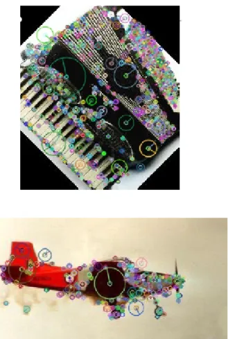
Unlike other histogram descriptors, SIFT algorithm does not give an overall im-pression of the image. Instead, it detects blob like features from the image and describes each and every point with a descriptor that contains 128 numbers. Point descriptors are given as output in the form of an array. Figure 3 shows accordion and airplane images and the SIFT keypoints detected on those. The radius of the circle on an image represents the strength of the keypoint.
2.2.3 Local Binary Patterns
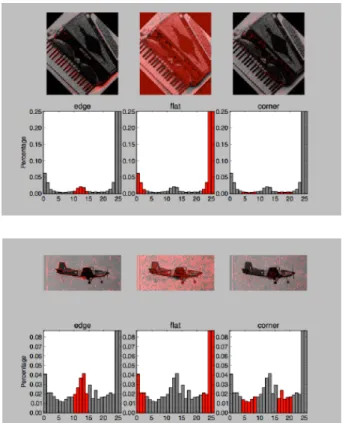
LBP [1] is a very efficient texture operator, it is a particular case of Texture Spec-trum model used for classification in computer vision. LBP labels the pixels of an image by segmenting the neighborhood of each pixel and considers the result as a binary num-ber. Since 1994, LBP has been found to be a powerful feature for texture classification. Detection performance on few datasets is improved drastically when LBP is combined with the Histogram of oriented gradients. In real-world applications, LBP is robust to monotonic gray-scale changes caused by different variations.
LBP is based on the Local Binary Patterns algorithm that has its roots in two-dimensional texture analysis. This algorithm works by comparing each pixel with its neighborhood and summarizing the local structure in an image. The comparison is done by taking a pixel as a center and threshold its neighbors against it. If the neighbor is greater or equal to the intensity of the center pixel, then center pixel is denoted with 1 and
Figure 4: Local Binary Pattern on Caltech-101 Dataset Samples
0. Hence, a binary number will be generated for each pixel. With 8 surrounding pixels, we will have28possible combinations. These combinations are called Local Binary Patterns or LBP codes. There are many extensions to these original LBP codes such as Extended LBP, also referred as Circular LBP. Figure 4 shows details like flatness, corners and edges of accordion and airplane images from Caltech-101 dataset.
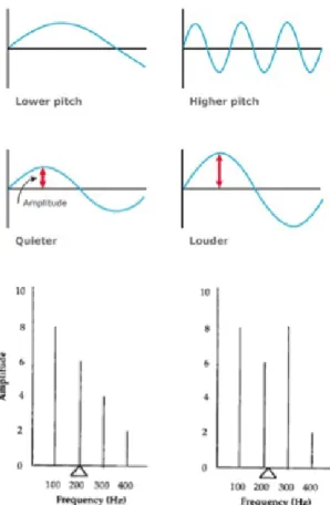
2.2.4 Audio Features
Similar to images, the grouped in k clustersaudio domain has several descriptive features. Figure 5 shows the basic features of audio domain. More features are discussed below.
1. Pitch: Pitch is an auditory sensation in which a listener assigns musical tones to relative positions on a musical scale based primarily on their perception of the fre-quency of vibration [13].
2. Energy: The sum of squares of the signal values, normalized by the respective frame length.
3. Spectral Centroid: It indicates where the ”center of mass” of the spectrum.
4. Mel Frequency Cepstral Coefficients: An acronym for MFCC, form a cepstral rep-resentation where the frequency bands are not linear but are distributed according to the mel-scale.
5. Chroma Vector: A 12-element representation of the spectral energy where the bins represent the 12 equal-tempered pitch classes of western-type music (semitone spacing).
2.3 Clustering
Clustering analysis is a function of grouping a set of data together in a way that data in the same group are analogous to each other than the data in other groups. It is a method of unsupervised learning and is a common technique used for the analysis of statistical data in various fields. K-means and SOM are two of such cluster analysis algorithms used to classify objects into K groups based on features of the object. K is considered as a positive integer. K-means are Self-Organizing Maps, which are described in detailed below, are used in generating SigSpaces to group similar features.
2.3.1 K-means
K-means is one of the simplest unsupervised learning algorithms. It was first originally developed for vector quantization. It is later applied to many other applications. Having the data and k as input, the data will be grouped into k clusters. Following is the algorithm for K-means:
Algorithm :
1. Let X =x1, x2, ..., xnbe the set of data points and V =v1, v2, ..., vcbe the set
of centers.
2. Randomly select ’c’ cluster centers.
3. Calculate the distance between each data point and cluster centers.
4. Assign the data point to the cluster center whose distance from the cluster center is minimum of all the cluster centers.
5. Recalculate the new cluster center using:
vi = (1/ci) ci X
j=1
xi
6. Recalculate the distance between each data point and newly obtained cluster cen-ters.
7. If no data point was reassigned then stop, otherwise repeat from step 3.
The same algorithm is applied to an image from Caltech-101 dataset from watch category, the centers are represented as red circles which can be seen in Figure 6.
Figure 6: K-means Centers(Red Circles) on Watch from Caltech-101 Dataset K-means being a popular algorithm in the Machine learning community, we shall discuss some of the pros and cons of the algorithm in detail.
Advantages:
1. It is fast, robust and easier to understand.
2. Relatively efficient: O(tknd), where n is the number of objects, k is the number of clusters, d is the number of dimensions of each object, and t is the number of iterations. Normally, k, t,d << n.
3. Gives the best result when the data set is distinct or well separated from each other. Disadvantages:
1. The learning algorithm requires apriori specification of the number of cluster cen-ters.
2. If there are two highly overlapping data, then K-means will not be able to resolve that there are two clusters.
3. The learning algorithm is not invariant to non-linear transformations. 4. Euclidean distance measures can unequally weight underlying factors.
5. Randomly choosing of the cluster center cannot lead us to effective results. 6. Applicable only when the mean is defined i.e. fails for categorical data.
7. Unable to handle noisy data and outliers. Algorithm fails for a non-linear data set. 2.3.2 Self-Organizing Maps
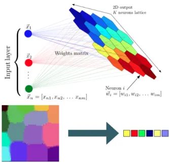
Kohonen Self Organising Feature Maps [5] [6] or SOMs were invented by Teuvo Kohonen, a professor of the Academy of Finland, and they provide a way of representing multidimensional data in much lower dimensional spaces - usually one or two dimensions. This process of reducing the dimensionality of vectors is essentially a data compression technique known as vector quantisation.
A common example used to help teach the principals behind SOMs [4] is the mapping of colors from their three-dimensional components - red, green and blue, into two dimensions. Figure 7 shows an example of a SOM trained to recognize the eight different colors shown on the right. The colors have been presented to the network as 3D vectors - one dimension for each of the colors components - and the network has learned to represent them in the 2D space. Notice that in addition to clustering the colors into distinct regions, regions of similar properties are usually found adjacent to each other.
Algorithm:
Select output layer network topology - Initialize current neighborhood distance, D(0), to a positive value. Initialize weights from inputs to outputs to small random values Let t = 1
Figure 7: Self-Organizing Map Use case with Colors 1. Select an input sample
2. Compute the square of the Euclidean distance of from weight vectors (wj) associated
with each output node
3. Select output node j* that has weight vector with minimum value from step 2.
4. Update weights to all nodes within a topological distance given by D(t) from j*, using the weight update rule
5. Increment t Endwhile
Advantages:
1. SOMs are very easy to understand.
3. If there is a black ravine between them, then they are different. Unlike Multidi-mensional Scaling or N-land, people can quickly pick up on how to use them in an effective manner.
4. They classify data well and then are easily evaluated for their own quality so you can actually calculate how good a map is and how strong the similarities between objects are.
Disadvantages:
1. SOM does not produce good results without proper data.
2. Unfortunately, each member of samples need a value for each dimension in order to generate a map.
3. It is very difficult to acquire all of the training data so this is a limiting feature to the use of SOMs often referred to a missing data.
4. Another problem is that every SOM is different and finds different similarities among the sample vectors.
5. SOMs organize sample data so that in the final product, the samples are usually surrounded by similar samples, however similar samples are not always near each other. If you have a lot of shades of purple, not always will you get one big group with all the purples in that cluster, sometimes the clusters will get split and there will be two groups of purple.
2.3.3 K-means vs SOM
We have used K-means and SOM for conducting all of our experiments, hence, comparing [7] K-means and SOM are not only necessary but also vital for understanding the minute details about them.
Comparisons
There is no need to specify the number of cluster centers for SOM, but K-means needs a priori specification of the number of clusters centers. SOMs classify data well and then are easily evaluated for their own quality. K-means classifies data if the clusters are well separated. Another problem is that every SOM is different and finds different similarities among the sample vectors. K-means gives similar clusters almost all the time given a specific configuration compared to SOM. SOM captures irregularities in the data well for data approximation goals. K-means, expects the clusters to be in spherical shape, thus, it cannot capture irregular shapes in data. SOM Time complexity = O(kmN), k = number of neurons, m = number of iterations, N = number of data points and Time K-means complexity = O(KlN), K = number of cluster centers, I = number of iterations, N = number of data points.
2.4 Supervised Classification Algorithms
Classification is one of the problems of machine learning that identifies the set of categories to which the instance belongs based on the training data set containing several observations whose category is known. In classification, the output variable takes class labels. Text categorization, fraud detection, optical character recognition, machine vision
Figure 8: Perceptron
are some of the examples of the classification problem. Classification is considered as an instance of supervised learning. All the algorithms listed below are used to test accuracy and training time. The accuracy and training times of these algorithms are compared with the approach used in SigSpace.
2.4.1 Perceptron
Perceptron [3] is a very basic unit in the neural network which can perform clas-sification of linearly separable patterns. The basic perceptron model is shown in Figure 8.
h() is the activation function, which performs decision based on the input.
h(
m
X
1
wx) = Output (2.1)
Activation FunctionsThere are different types of activation function. Learning Algorithm
1. Initialization set all of the weightswij to small (positive and negative) random
num-bers
2. Training for T iterations or until all the outputs are correct: 3. Recall
2.4.2 Decision Tree
Decision tree [10] is a popular method for machine learning tasks like classifica-tion and regression. They are widely used to handle the categorical features and easily scaled to multiple class classification. They are easy to understand and explain to others. The model is a group of regions which are rectangular in shape.
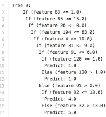
Figure 9 shows a sub tree with branches of ’if’ and ’else’ which is generated from Caltech-101 with 6 classes. The original tree consists a depth of 8 and 397 nodes.
2.4.3 Random Forest
Random forest [10] Method uses multiple learning algorithms to predict better based on the past observations. This is used for regression and classification and few other tasks. Random forest operates by constructing a large number of decision during the training and gives individual trees, mode of all the classes or predicts the mean as an output. Figure 10 shows part of one of the Trees.
Figure 10: Random Forest Classifier 2.4.4 Naive Bayes
Naive Bayes technique is a supervised classification algorithm. It is based on Bayes theorem [2.2] to train the dataset. It generates the models to identify the relation between input data and the predictable data. The features are considered as independent. The probability of test data is generated irrespective of their correlation.
P(θ|D) = P(θ)P(D|θ)
P(D) (2.2)
2.5 Bag of Visual Words
The image classification can be rendered by creating a bag of visual words [12] which is prominently called as bag-of-words model. This process treats image features
Figure 11: Visual Words
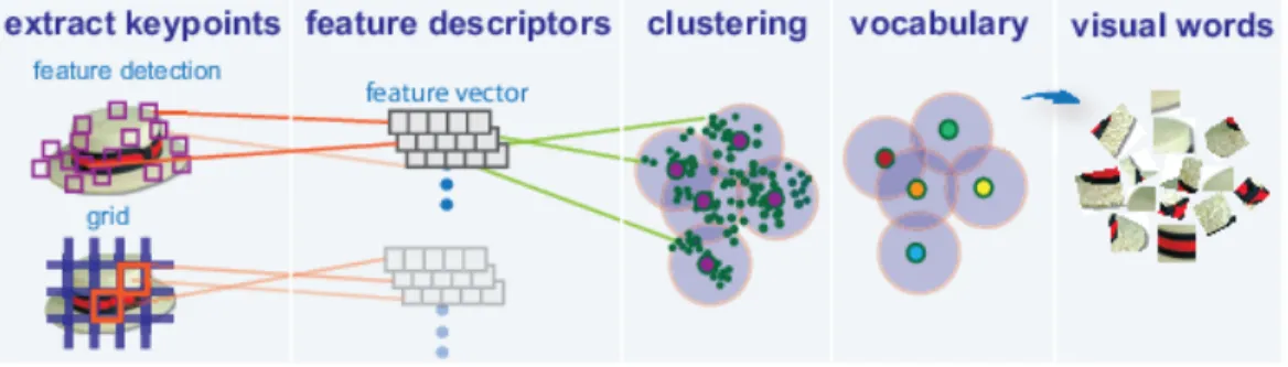
as words and generates a histogram of visual word occurrences that represent an image. Figure 11 exactly depicts the process of generating visual words. These histograms are used to train an image category classifier.
The first step is to organize and partition the images into training and test subsets. The second step is to create a visual vocabulary or bag of features by extracting feature descriptors from representative images of each category. The k-means clustering algorithm is used to define the features or visual words of bag-Of-Features object. This algorithm is used on the feature descriptors extracted from training sets.
The feature descriptors are iteratively grouped into k mutually exclusive clusters which are separated by similar characteristics. The visual word or the feature corresponds to the center of each cluster. This algorithm uses ’grid’ method for images which provides greater scale invariance without any distinct features to extract feature descriptors. Grid method should always be used for images that do not contain distinct features like the beach. Approach: The images were analyzed entirely using this algorithmic workflow. The workflow neither relies on spatial information nor on marking the particular objects in an image. The bag-of-visual-words technique relies on detection without localization.
Figure 12: Encode Overview
The third step is to train an image classifier with a bag of visual words. This helps in encoding the images in the image set using a bag of visual words into the histogram of visual words which are then used as the positive and negative samples to train the classifier. Figure 12 shows the process of encoding an image to feature vector.
1. The bag-Of-Features is used to encode each image from the training set by approx-imating nearest neighbor algorithm after detecting and extracting the features from the image. This algorithm helps to construct a feature histogram for each image. 2. The above step is repeated for all the images of the training set to create training
data.
3. Then test the quality of the classifier against the validation image set. A confusion matrix is used to predict the results.
2.6 Principal Component Analysis
Principal component analysis [9] identifies the patterns in the data and reduces the dimensions of the data with minimal loss of information and brings the strong patterns of
Figure 13: Two Dimensional Space with 2 Principal Components
the data sets. It uses orthogonal transformations to convert the sets of correlated variables of data to uncorrelated variables which are called principal components. Figure 13 shows the two principle components.
It uses the eigenvectors and eigenvalues to determine the principal components. After getting a set of data points, it deconstructs eigenvectors which represent directions. Each eigenvector has eigenvalue which provides the variance in the data sets in that direc-tions. These eigenvalues determine how the data is spread across,the eigenvectors with maximum eigenvalues are the principal components. PCA is used for predictive models and are mainly used in exploratory data analysis.
Algorithm:
1. Take the whole dataset consisting of dd-dimensional samples ignoring the class labels
2. Compute the dd-dimensional mean vector (i.e., the means for every dimension of the whole dataset)
set
4. Compute eigenvectors(e1, e2, ...., ed)and corresponding eigenvalues(λ1, λ2, ..., λd)
5. Sort the eigenvectors by decreasing eigenvalues and choose kk eigenvectors with the largest eigenvalues to form a dxk dimensional matrix W (where every column represents an eigenvector)
6. Use this dxk eigenvector matrix to transform the samples onto the new subspace. This can be summarized by the mathematical equation: y = WT ∗x (where x is
a dx1-dimensional vector representing one sample, and y is the transformed kx1-dimensional sample in the new subspace.)
2.7 Vector Space Model
Vector space modelling is one of the information retrieval model that is widely ap-plied in evaluation of web search engines. This model represents queries and documents as vectors in multidimensional space. The similarity values between a given query and a set of documents are computed by the cosine similarity function of retrieval operations. The documents are ranked based on this relevance called relevancy rankings, and they can be used in the evaluation of web search engines.
The vector space model procedure can be divided into three stages: 1. The first stage is the document indexing where content bearing terms are extracted from the docu-ment text. 2. The second stage is the weighting of the indexed terms to enhance retrieval of the document relevant to the user. 3. The last stage ranks the document with respect
to the query according to a similarity measure. A common similarity measure known as cosine measure determines the angle between the document vector and the query vector as described above.
The cosine angle is used to compute the numeric similarity, and is used to deter-mine the angle between the document vector and query vector when they are represented in V-dimensional Euclidean space where V denotes the size. The similarity function be-tween the document vector and query vector is given by
cosθ =Similarity(Di, Q) = Di·Q ||Di|| · ||Q|| where Di is the Document vector, Q is Query.
The vector space model has several properties that are attractive. Compared to other hand-coded knowledge bases and ontologies, the vector space model extract knowl-edge automatically from a given corpus, thus requiring lesser labor than other approaches. It has interesting relation especially with the distributional hypothesis and related hypoth-esis. The distributional hypothesis is that words that occur in similar contexts tend to have similar meanings. Efforts to apply this abstract hypothesis to concrete algorithms for mea-suring the similarity of meaning often lead to vectors, matrices, and higher-order tensors. This intimate connection between the distributional hypothesis and vector space models is a strong motivation for taking a close look at them. This general hypothesis underlies several more specific hypotheses, such as the bag of words hypothesis, the distributional hypothesis, and the extended distributional hypothesis.
2.8 Summary
Classification in the fields of computer vision, audio analysis etc., is on the fore-front as it has many applications in real time. It can be improved from simply using pixels data in images to classify the data to machine performing highly complex tasks.
Machine learning decisions have moved from high processing machine to com-modity hardware and then to smartphones which are low processing devices. The de-cisions should be taken in a very less time, hence, we propose the SigSpace to support the properties mentioned above and validate its performance with respective the other machine learning algorithms. Even though the experiments are done on four kinds of fea-tures and two kinds of clustering algorithms, we leave the other evaluations for the future work to get a detailed report.
CHAPTER 3
PROPOSED SOLUTION : SIGSPACE 3.1 Introduction
In the previous chapter, we have built the bridge between the state of art method-ologies and SigSpace. In this chapter, we will discuss SigSpace architecture and the SigSpace models formed using different features: Pixels, Scale invariant feature trans-form, Local binary patterns and audio features. We will also discuss how matching and fuzzy matching works using SigSpaces.
3.2 SigSpace Models
SigSpace is a novel architecture inspired by the field of Statistics on how the sum-mary of data is captured using simple measures. Referring to the quote”A picture speaks a thousand words”, the image has more information and with more information comes more noise. World is full of patterns, as defined by Cambridge Dictionary a pattern is”any regularly repeated arrangement, especially a design made from repeated lines, shapes, or colors on a surface”. The features can be clustered to form a better summarized group of elements, which forms the basis for ”SigSpace”.
We present the objectives of our SigSpace architecture as follows:
1. Dimension reduction of data: It is a known fact that good data is key to a good model. The SigSpace is reduced form of data space, which occupies less than 10%
of the data space.
2. Time complexity: The training time taken by a machine learning algorithm is lim-ited compared to the time taken in learning the data space which is very larger than SigSpace. Hence, using SigSpaces reduces the time.
3. Distributed learning: The SigSpace architecture is implemented on big data pro-cessing tool which is distributed in nature, as classes are independent of each other, it is possible to generate and learn the SigSpaces distributively.
4. Incremental learning: SigSpaces will learn the data using incremental clustering algorithms: K-means and SOM.
5. Fuzzy classification: The SigSpace matching approach matches the test data over multiple SigSpaces which gives the probabilistic scores over a couple of them. This makes it possible to get closest classes for the classification task.
6. Reusability: Once SigSpaces have generated the models, it occupies very less space compared to what the original data occupies, and it can be easily transferred to any device to perform predictive analysis.
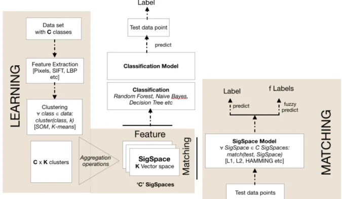
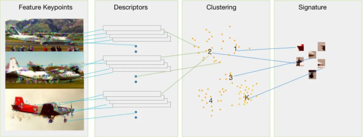
The proposed architecture is shown in Figure 14. It consists of two essential modules, SigSpace Learning and SigSpace Matching. As shown in the same figure, the SigSpace models formed can also be used as features for classification algorithms. The evaluations of SigSpaces as features are shown in Chapter 4.
SigSpace Learning: This is first module in the architecture and it consists of multiple steps:
1. Feature Extraction: From the dataset, different kinds of features are extracted. In the current approach, Pixels, SIFT, LBP and Audio features are extracted.
2. Clustering: The features extracted/generated from the previous step is clustered per class using K-means of SOM clustering algorithms. The output of K-means are the centroids, but SOM gives out group for which we have to explicitly find the centroids.
3. Aggregation: The clusters formed using the above step can be used to find various central tendency measures. In the current approach, we are concentrating on mean. 4. SigSpace: For each class, the mean vectors are generated. Which forms SigSpace
correspondent to a class.
SigSpace Matching: This module works similar to what classification algorithms does. After generation of SigSpaces using SigSpace Learning, features from the test file/object are extracted and they are matched with each SigSpace to get the dissimilarity score using L2 Norm. Section 3.5 discusses more about the approach.
Figure 15 shows SigSpaces for ten different classes from the dataset MNIST that is generated using the Algorithm 1. Using the same algorithm, the SigSpaces for Accordion and Airplanes from Caltech-101 data are generated with 100 clusters are shown in Figures 16, 17 and 18.
Figure 14: SigSpace Architecture
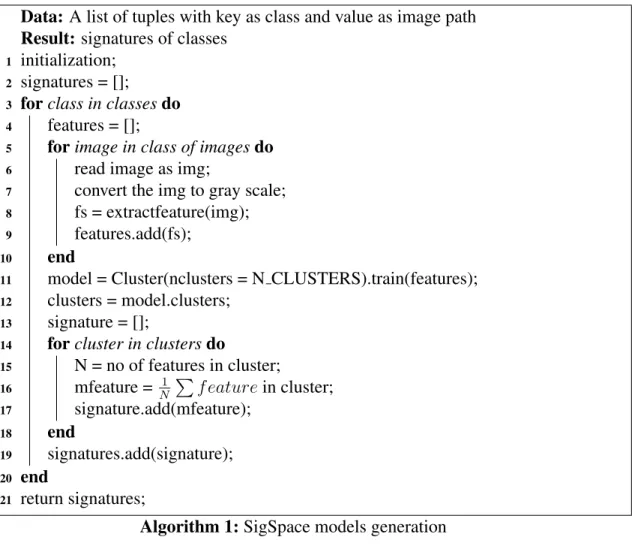
Data: A list of tuples with key as class and value as image path Result: signatures of classes
1 initialization; 2 signatures = [];
3 forclass in classesdo 4 features = [];
5 forimage in class of imagesdo 6 read image as img;
7 convert the img to gray scale; 8 fs = extractfeature(img); 9 features.add(fs);
10 end
11 model = Cluster(nclusters = N CLUSTERS).train(features); 12 clusters = model.clusters;
13 signature = [];
14 forcluster in clustersdo
15 N = no of features in cluster;
16 mfeature = N1 Pf eaturein cluster; 17 signature.add(mfeature);
18 end
19 signatures.add(signature); 20 end
21 return signatures;
Algorithm 1:SigSpace models generation
Figure 17: Caltech-101, Accordion SigSpace with k = 100
3.3 SigSpace Learning
The data in real world has patterns and that is how humans learn to distinguish or recognize the objects. SigSpace finds important patterns that are defined as a structure regularly repeated. Clustering makes sense whenever there are a group of similar items as it is used to capture the central tendency of the distribution. SigSpace learning follows generative model approach. The key features of the classes are learned and modeled. Figure 19 shows the generation of class based SigSpace.
The Algorithm 1 is divided into 4 submodules and the details are listed as follows: 1. Feature extraction: when a dataset of images, audio files or raw data are given to build a Machine learning model, features are the first things to move forward to the training process.
2. Clustering: Cluster the features extracted in the previous step on a class based manner. In the experiments K-means and SOM are used for clustering.
3. Aggregation: In each class for each cluster, aggregate the features using some mea-sure of central tendency. In our experiments, we have used mean. Other meamea-sures like median, mode, medoid etc., are left for future work.
4. SigSpace generation: Collect the aggregated features as vectors per class, which becomes the SigSpace per class.
Figure 19: SigSpace Model Generation 3.4 SigSpace as Feature for Classification
As already discussed in Chapter 2, features are vital for training Machine learning models. Keeping aside the vital purpose of SigSpace, it can also be used as feature set. Using SigSpaces for classical Machine learning algorithms is very well fitting, because the number of data points to be learned is very few compared to the original feature space and the time required to train the model is very less compared to that of the original features. The comparisons are shown in Chapter 5.
Figure 19 shows the step where SigSpace is used as features for Classification algorithms like Random Forest, Naive Bayes, Decision Tree and Perceptron etc.
In this context, the SigSpaces can be used to build on-demand models for mobile devices, where they would not have capabilities to generate models based on big data but can use the SigSpaces and generate equally performing models.
3.5 SigSpace Matching
Instead of using the classification algorithms, SigSpace Matching can be used. The foremost theory behind SigSpace matching is Class-based Matching. The models generated will be reused to match the test data points and get a measurement of dissimi-larity. Based on the measurement, the top ’f’ similar classes is chosen which is defined as Fuzzy Matching.
3.5.1 Measuring Similarity
Determining how similar two images/objects are, is a fundamental task for any Classification algorithms. The most commonly used measures which provide a numeric measure describing how similar two vectors/objects are listed below:
1. L1 Norm (Manhattan distance): It is sum of absolute values of horizontal and ver-tical distances. It is suited for features like Pixel and SIFT.
Pn
i=1|xi−yi|
2. L2 Norm (Euclidean distance): It is distance between points or vectors measured using Pythagoras’ theorem. In our experiments this is well suited for Pixels and SIFT features.
pPn
i=1(xi−yi)2
3. Hamming Distance: It is very similar to Manhattan distance with an exception that the features are in binary. This is well suited for Binary features.
Pn
In the case of matching a test data point with Class, the dissimilarity is calculated using one of the measurements listed above. The SigSpace with less dissimilarity will be elected as the resultant class. It is possible to generate closest ”c” classes that a test data point/space belongs to. Figure 20 shows an image, in this case a watch image from Caltech-101 dataset, is used as a test image to match using SigSpaces Airplane and Watch. More detailed illustration is shown in Figure 21. SigSpace model, as shown in the figure, is a vector space model, where each class SigSpaces are projected in n-dimensional space and the test features are projected as well and the dissimilarities are calculated.
L1 vs L2 Norms: For all the experiments we used L2 norm because of the fol-lowing experiment. For better illustration, the two images, Figure 22 shows L1 norm matching and Figure 23 shows L2 norm matching. The qualitative analysis has showed that L2 matching is better than L1.
3.5.2 SigSpace Graph Matching
To reduce the complexity of comparison, construct a graph of SigSpaces with dissimilarities between them as the edges. To match a test data point on to the SigSpace Model, Select a random node from the graph and match the edges to the most similar nodes, this reduces the comparison from all the nodes to some of them. Hence decreases the matching time exponentially.
Algortihm 2 gives the function to generate Graph from SigSpaces and Algorithm 3 gives detail for matching, which can be extended to fuzzy matching.
Figure 21: SigSpace Matching on Vector Space
Figure 23: L2 Matching
Data: A list of SigSpaces Result: Graph G of SigSpaces
1 initialization; 2 c = no of classes;
3 D = dissimilarity matrix of size cxc;
4 dij = dissimilarity between SigSpace i and j; 5 Si = SigSpace of class i; 6 forciin classesdo 7 forcj in classesdo 8 D[i, j] = dissimilarity(ci,cj); 9 end 10 end
11 Construct graph G with c nodes with Adjacency matrix D.; 12 return G;
Data: Graph G of SigSpaces, Test data point as test Result: label
1 initialization; 2 c = no of classes;
3 D = dissimilarity matrix of size cxc;
4 dij = dissimilarity between SigSpace i and j; 5 Si = random(c);
6 d = dissimilarity(test,Si); 7 matches = [];
8 GI < V, EI >= getSubGraph(G < V, E >, d,Si); 9 matches = dissimilarity(GI, test);
10 label = min(matches); 11 return label;
Algorithm 3:SigSpace Matching
Figure 24 shows the step by step visualization for graph matching.
1. Step 1: The Graph with dissimilarities are shown with green showing similar and red as different.
2. Step 2: Select the test data point[s] and Random Node, in this case t andS1.
3. Step 3: Now find the dissimilarity between random pointS1 and t.
4. Step 4: Based on the measurement, sub graph is selected, in the image we can see the subgraph consists ofS1 andS4.
5. Step 5: Finally select closest one from the subgraph. In the example the labelS4 is
3.6 SigSpace Fuzzy Matching
Fuzzy Matching uses the same basis of SigSpace Matching, the only difference is that instead of selecting a class with the minimum dissimilarity, in Fuzzy Matching, ”f” classes with minimum dissimilarity measure are selected.
For example, considering the dataset MNIST, the workflow is shown in Figure 25. A test image that belongs to class 7 is given to predict using Fuzzy matching. In the first step, the pixels are extracted, then Fuzzy match algorithm is employed to calculate the dissimilarity using L2 norm or Euclidean distance, normalizing the measure, the confi-dence scores are calculated as shown in the figure. The result from Fuzzy Matching with f=2 (selection criteria) are 7 and 2. In case of bad features without much variance, fuzzy matching gives out almost equal dissimilarity for all of the classes.
3.7 Summary
Information presented in this chapter suggests that SigSpace approach solves achieves the properties like independence, capability to distributively learn, fuzziness in predic-tions etc.
SigSpaces are closer to actual data, as observed in the usecase of MNIST dataset, SigSpaces of the numbers looked very similar to the actual digit images from the dataset. Using shallow architecture, SigSpace architecture, it is possible to get a high level feature representations. Much needs to be done in the way prediction is being done, but as already proposed, the Graph approach will reduce the time complexity of matching.
CHAPTER 4
IMPLEMENTATION AND EVALUATION 4.1 Introduction
This chapter describes several sets of evaluations that were conducted using SigSpace. Implementation, System configurations will also be discussed. The experiments were de-signed to verify factors like training time taken by SigSpace compared to the state of art machine learning algorithms, space occupied by normal features vs SigSpaces, the accu-racy of the state of art algorithms compared to SigSpaces and Fuzzy matching approach compared with SigSpace matching.
4.2 Implementation
Apache Spark framework is used to conduct all the experiments on Unix File System or HDFS.
4.2.1 Apache Spark
Apache Spark is a cluster computing platform which has been designed to be fast. Figure 26 shows the modules of Spark architecture. Spark extends map reduce to support more types of computations, Interactive queries and stream data processing. It provides high-level APIs in Java, Scala, Python and R, and an optimized engine that supports general execution graphs.
It also supports a rich set of higher-level tools including Spark SQL for struc-tured data processing and using SQL and Apache Hive. The Spark streaming is a spark package which process the live streaming data. MLlib package of spark provides com-mon Machine Learning algorithms like classifications, regressions, collaborative filtering for machine learning, GraphX package of spark provides API for graph manipulations. Spark has designed to scale up on thousands of nodes in order to achieve this flexibility it supports different cluster managers like Apache Mesos, Hadoop YARN. Spark computes distributed datasets on the files stored in the file system. Even if the dataset is lost it is recomputed using Lineage graphs. These RDD’s supports two operations named trans-formations and actions. Transtrans-formations produce new RDD’s whereas the actions bring the results back to the driver programs. Spark framework has built-in functions such as parallel processing, distributed computing etc. As we have tested the SigSpace using Spark, the objectives such as distributed processing and independent learning are already achieved.
4.2.2 Tools
The tools which were used to achieve the experiment were described below. 1. OpenCV: OpenCV is an image processing framework which is released under a
BSD license and it’s free for both academic and commercial use. It has C++, C, Python and Java interfaces and supports Windows, Linux, Mac OS, iOS and An-droid. OpenCV was designed for computational efficiency and with a strong focus on real-time applications.
Figure 26: Apache Spark Architecture
2. scikit-learn: Scikit-learn is a machine learning library for the Python programming language used for mining and analysis of data. It features various algorithms like classification, regression and clustering along with random forests, k-means, and gradient boosting. It is designed to be used with python libraries SciPy and NumPy. It provides consistent interface to machine learning models which makes it easy to learn the usage of a new model. It provides many options to each model to tune them for optimal performance but with sensible defaults.
Scikit provides rich set of functionality for companion tasks like model selection, model evaluation, and data preparation. It is under active development and under active community on stack overflow for development and support.
3. scikit-image: Now a days, images are the most voluminous source of data. In our data rich world, images represent an essential subset of all the analysis made. Ex-amples include robotic vision capture, satellite maps, and other higher dimensional
images. Exploring these date resources needs widely distributed and well-formed tools that should be easy to use and be able to address significant challenges in various fields of analysis.
Scikit-image, a library used for image processing in the Python programming lan-guage. It is considered as one of the complementary tools to produce high quality, well documented and adaptable implementation of image processing algorithms. It is available under the open source license of liberal BSD. It implements algorithms and utilities for its use in education, research and industrial applications. The library allows developers in image processing to learn algorithms efficiently with minimal adjustments and modification to the code.
4. Core Audio Framework: Core Audio Framework is a framework in iOS. It is used to analyze audio files.
4.3 Datasets
4.3.1 MNIST
The MNIST (Figure 27) consists of handwritten digits, has a training set of 60,000 examples, and a test set of 10,000 examples. It is a subset of a larger set available from NIST. The digits have been size-normalized and centered in a fixed-size image.
4.3.2 Caltech-101
It is a data set of digital images (Figure 28) It is applicable for techniques involving image recognition classification and categorization. The caltech-101 data set contains
Figure 27: Samples from MNIST Dataset
Figure 28: Samples from Caltech-101 Dataset
a total of 9,146 images, split between 101 different object categories and each object category contains between 40 and 800 images. Most categories have about 50 images and the size of each image is roughly 300x200 pixels.
4.3.3 Caltech-256
Caltech-256 (Figure 29) images are harvested from two popular online image databases that represent a diverse set of conditions and systematics. This data set contains 256 object categories and clutter with at least 80 images per category. The caltech-256
Figure 29: Samples from Caltech-256 Dataset
data set contains a total of 30608 images with a maximum of 827 pictures per category. 4.3.4 UEC FOOD 256
UEC Food 256 data set(Figure 30) contains 256-kind food photos. This data set was built to implement a practical food recognition system in Japan and hence, most of the food categories in this data set are popular foods in Japan. Each food photo of this data set has a bounding box indicating the location of the food item in the photo.
4.3.5 ImageNet
ImageNet(Figure 31) is an image database organized according to the WordNet hierarchy, in which each node of the hierarchy is depicted by hundreds and thousands of images. At present there are 1000 categories with more than a million images.
Figure 30: Samples from UEC FOOD 256 Dataset
4.4 Results and Evaluation
Four case studies were taken to observe the SigSpace behaviour. Following are the case studies.
1. Image Classification with Pixels: In this experiment, Pixels are extracted from MINST dataset to evaluate accuracy, model training time and space occupied by feature and SigSpaces. Perceptron algorithm is used for classification. It is com-pared with SigSpace.
2. Image Classification with LBP: In this experiment, LBP features are extracted from Caltech-101 dataset to evaluate accuracy and model training time and Space oc-cupied by features and SigSpaces. Random Forest is used for classification. It is compared with SigSpace.
3. Image Classification with SIFT: In this experiment, top 500 strong SIFT features are extracted from the images of Caltech-101 and Caltech-256 datasets. Naive Bayes, decision tree, random forest are used and compared with SigSpace.
4. Audio Classification:
Dataset: Audio dataset (Real-time) Decision Tree vs SigSpace
Performance (accuracy and model training time) and Space
We have worked with different datasets like Caltech 101, Caltech 256, UECFOOD 256, ImageNet and MNIST.
4.4.1 Case 1: Image Classification with Pixels
The objective of this experiment is to test the training time and space complexity of SigSpace over a low level feature named pixels compared.
• Dataset: MNIST (handwritten digits) • Training set: 60,000 images
• Test set: 10,000 Images
• Algorithm: Deep Learning with softmax regression and Conjugate Gradient learn-ing mechanism.
• SigSpace: K-means and SOM Case 1: Evaluation
As can be seen in Figures 32 and 33, the model training time and space using SigSpace is better than the classification algorithm. The classification algorithm used here is Deep Learning with softmax regression and Conjugate Gradient learning mechanism which achieved an accuracy of 92.04%. The SigSpace generated using Self-Organizing Map achieved an accuracy of 87.86% with just 3% of data. SigSpace generated using K-means achieved an accuracy of 87.2% with 1% data-based clustering. In terms of space, the data space is reduced from 60,000 to 300. Deep Learning approach took 120 minutes and SigSpace took a maximum of 4 minutes to achieve the maximum accuracy of 87.86%.
4.4.2 Case 2: Image Classification with LBP
In this case study, a global image feature named Local binary pattern is used to generate SigSpace and compare the training time and space complexity of few classifica-tion algorithms with SigSpace.
• Feature: LBP (Local binary patterns) • Dataset: Caltech-101
• Training set: 6403 • Test set: 2743
• Algorithms: Random Forest, Decision Tree and Naive Bayes • SigSpace: K-means and SOM
Case 2: Evaluation
The results are illustrated in Figures 34 and 35. Random Forest, Decision Tree and Naive Bayes are used to evaluate the performance and Random Forest has performed best with an accuracy of 57.83%. SigSpace is generated using K-means and SOM. Us-ing SigSpace with SOM, the accuracy is observed to be 52.40% with K=50% data-based clustering. The SigSpace formed using K-means clustering seems to under perform com-pared to SOM. The training time for SigSpace generated using K-means is lesser than SOM. And, the training time for non-SigSpace method falls within the intervals of K-means and SOM.
Figure 34: Random Forest vs. SigSpace Space Reduction and Performance
Figure 36: Number of Data Points 4.4.3 Case 3: Image Classification with SIFT
In this case, local image feature named Scale-invariant feature transform is used to generate SigSpace. The model training time, space complexity and classification accuracy are observed.
SIFT features are extracted on Caltech 101, Caltech 256, UEC 256, ImageNet -ILSVRC datasets. Figure 36 shows number of datapoints generated per dataset and Figure 37 shows the time taken to extract SIFT features on each of those dataets. Random Forest, Decision Tree and Naive Bayes are used for classifying and K-means and SOM are used for generating SigSpaces.
Figure 37: Number of Hours to Extract SIFT
Gigabytes over datasets Caltech-101, Caltech-256, UEC FOOD 256 and ImageNet. Case 3-2: SigSpace Fuzzy Matching
A sample of 6 classes are randomly chosen from Caltech-101 dataset. SIFT fea-tures are extracted from the images and SigSpace with k=20% data-based clustering is done. Classification accuracy is observed using Random Forest, SigSpace Matching and Fuzzy Matching. The accuracies are listed below:
Random Forest - 17.81% SigSpace Matching - 17%
SigSpace Fuzzy Matching - 15.82%
Figure 38: Raw Data vs SIFT vs SigSpace
precision on a whole compared to the normal matching. For example, the accordion class accuracy is improved in Fuzzy matching compared to the SigSpace Matching approach.
Case 3: EvaluationAs shown in the Figures 38 and 42, using SIFT for a classifi-cation task has not performed well. However, it is necessary to know that SigSpace still performs close to classification algorithms with an accuracy difference of 0.81%. Con-sidering the confusion matrix of Fuzzy Matching in Figure 39, the class distribution is improved when compared to SigSpace Matching. For example, the first class in SigSpace Matching has 0 predictions whereas Fuzzy Matching got 3.48 predictions. This explains that Fuzzy Matching boosts the performance of under performing classes compared to SigSpace Matching.
Figure 39: Confusion Matrices: SigSpace Matching and Fuzzy Matching
Figure 41: Confusion Matrix: Fuzzy SigSpace Matching 4.4.4 Case 4: Audio Classification
In this case study, we will experiment with audio domain features to generate SigSpace. The objective of this experiment is to compare factors like model training time and space complexity of SigSpace with classification algorithms. The experiment is conducted using real-time data, all the audio data is collected using an iOS device in several contexts and transferred to Spark server as audio files. The machine learning models are generated on the server by extracting several features like pitch, loudness, MFCC, spectral centroid etc., from the audio files. 5,959 audio files are used for training and 1787 audio files for testing the models. In the present evaluation, household context is used. The classification models are generated using decision tree and random forest
Figure 43: Supervised Learning vs. SigSpace Accuracy and Space Reduction and the SigSpace is generated using SOM.
Case 4: EvaluationAs can be seen in Figure 43, unlike all the other experiments, decision tree performed better than random forest. The accuracy of decision tree and ran-dom forest are listed below: Decision Tree: 82.2% Ranran-dom Forest: 80.6% SigSpace(Self-Organizing Maps): 81.5% with 3.3% data-based clustering
Figure 44 shows that as the SigSpace size increases the training time increases. The maximum accuracy obtained using SigSpace 3.3% (training set is reduced from 5959 to 200) data-based clustering took only 25 secs to train the model whereas the decision tree model took 70 secs to train the same.
4.5 Summary
The results from the experiments clearly indicate that SigSpace is absolutely better than the state of art algorithms in time and space factors, with a slight decrease in accuracy which is understandable. We are not interested in producing high accuracy SigSpace mod-els. Rather, we are interested in the tests which can tell us the performance of SigSpace compared to the state of art algorithms and methodologies in a quantitative and qualitative manner. There is still room for improvement in some of the components of the architec-ture and is open for discussion. The fuarchitec-ture work and improvements are discussed in detail in the next chapter.
CHAPTER 5
CONCLUSION AND FUTURE WORK 5.1 Conclusion
The thesis presented a novel approach to build models that has unique capabilities like independent learning, distributed learning, fuzzy matching etc. This approach differs from the existing approaches considering the above factors. Although, there has been a slight accuracy decrease (approximately 5%) in the overall performance, SigSpace is very efficient, in terms of space as well as run time performance for learning and recognition. The present evaluation thus confirms SigSpace as an important approach for distributed and scalable machine learning with big data.
5.2 Future Work
There are some practical and theoretical concerns that need to be addressed. So, though we have promising results in the factors like space and time complexity, much future work remains.
Dissimilarity Measures: Using mean as the central tendency measure, we would like to test matching with other measures like median, medoid, mode etc. In the case of calculating dissimilarity, we need to experiment on other measures like Cosine similarity, Manhattan distance.
SigSpace, which is entirely based on the features used, but the recognition problem has a huge range of features that needs to be addressed. For example, the food domain needs both shape and color features to recognize a food item rather than just one of them. Thus, Multiple SigSpaces must be designed to outperform classic classification algorithms.
Multilevel SigSpaces:Metadata of SigSpaces can be used for better matching of SigSpaces with test data. Multilevel SigSpaces can even help SigSpaces to be organized hierarchically to help very large scale classification/recognition problems which are hard to be solved.
This work helped us expand our understanding of the machine learning with data reduction, independent learning, distributed learning and fuzzy matching.
REFERENCE LIST
[1] Local binary patterns - scholarpedia. http://www.scholarpedia.org/ article/Local_Binary_Patterns. (Accessed on 06/09/2016).
[2] Machine learning - wikipedia, the free encyclopedia. https://en. wikipedia.org/wiki/Machine_learning. (Accessed on 04/12/2016). [3] Perceptron - wikipedia, the free encyclopedia.https://en.wikipedia.org/
wiki/Perceptron. (Accessed on 04/11/2016).
[4] Self-organizing maps. http://davis.wpi.edu/˜matt/courses/soms/. (Accessed on 04/11/2016).
[5] Som tutorial part 1.http://www.ai-junkie.com/ann/som/som1.html. (Accessed on 04/11/2016).
[6] Som.pdf. https://genome.tugraz.at/MedicalInformatics2/SOM. pdf. (Accessed on 04/11/2016).
[7] CHEN, Y., QIN, B., LIU, T., LIU, Y., AND LI, S. The comparison of som and
k-means for text clustering. Computer and Information Science 3, 2 (2010), 268. [8] DINAKARPANDIAN, D. Mitigating high dimensionality in big data analysis. Big
Data Analysis for Bioinformatics and Biomedical Discoveries(2016), 249. [9] FODOR, I. K. A survey of dimension reduction techniques, 2002.
[10] JAMES, G., WITTEN, D., HASTIE, T., AND TIBSHIRANI, R. An introduction to statistical learning. vol. 112. Springer, 2013, pp. 303–335.
[11] KANG, G. Digital image processing. Quest, vol. 1, Autumn 1977, p. 2-20. 1(1977), 2–20.
[12] MATLAB. Image classification with bag of visual words - matlab & simulink. http://www.mathworks.com/help/vision/ug/ image-classification-with-bag-of-visual-words.html.
(Accessed on 04/12/2016).
[13] PLACK, C. J., OXENHAM, A. J., AND FAY, R. R. Pitch: Neural Coding and Perception, vol. 24. Springer Science & Business Media, 2006.
VITA
Seetha Rama Pradyumna Doddala was born on June 2, 1990 in Guntur, Andhra Pradesh, India. He was educated in local public schools and graduated from University of Missouri-Kansas City in 2016 at an age of 26. Before proceeding to Graduate studies, he has a 4 year work experience in few IT companies concentrating on Mobile appli-cation development in Life sciences, Entertainment domains. While he was studying in UMKC, he has worked as Graduate Teaching Assistant for Big data Apps and Analytics and Advanced Software Engineering courses.