Improving group role assignment problem by incremental assignment algorithm

(1)

Improving Group Role Assignment Problem By Incremental Assignment Algorithm

by

Pinzhi Wang

A thesis submitted in partial fulfillment of the requirements for the degree of

Master of Science (MSc) in Computational Sciences

The Faculty of Graduate Studies Laurentian University Sudbury, Ontario, Canada

(2)

ii

Faculty of Graduate Studies/Faculté des études supérieures Title of Thesis

Titre de la thèse Improving Group Role Assignment Problem By Incremental Assignment Algorithm Name of Candidate

Nom du candidat Wang, Pinzhi

Degree Diplôme Master of Science

Department/Program Date of Defence

Département/Programme Computational Sciences Date de la soutenance October 29, 2019

APPROVED/APPROUVÉ Thesis Examiners/Examinateurs de thèse:

Dr. Youssou Gningue (Supervisor/Co-directeur de thèse) Dr. Haibin Zhu (Co-Supervisor/Co-directeur(trice) de thèse) Dr. Matthias Takouda

(Committee member/Membre du comité)

Approved for the Faculty of Graduate Studies Approuvé pour la Faculté des études supérieures Dr. David Lesbarrères

Monsieur David Lesbarrères Dr. Dongning Liu Dean, Faculty of Graduate Studies (External Examiner/Examinateur externe) Doyen, Faculté des études supérieures

ACCESSIBILITY CLAUSE AND PERMISSION TO USE

I, Pinzhi Wang, hereby grant to Laurentian University and/or its agents the non-exclusive license to archive and make accessible my thesis, dissertation, or project report in whole or in part in all forms of media, now or for the duration of my copyright ownership. I retain all other ownership rights to the copyright of the thesis, dissertation or project report. I also reserve the right to use in future works (such as articles or books) all or part of this thesis, dissertation, or project report. I further agree that permission for copying of this thesis in any manner, in whole or in part, for scholarly purposes may be granted by the professor or professors who supervised my thesis work or, in their absence, by the Head of the Department in which my thesis work was done. It is understood that any copying or publication or use of this thesis or parts thereof for financial gain shall not be allowed without my written permission. It is also understood that this copy is being made available in this form by the authority of the copyright owner solely for the purpose of private study and research and may not be copied or reproduced except as permitted by the copyright laws without written authority from the copyright owner.

(3)

iii

Abstract

The Assignment Problem is a basic combinatorial optimization problem. In a weighted bipartite graph, the Assignment Problem is to find a largest sum of weights matching. The Hungarian method is a well-known algorithm which is combinatorial optimization.

Adding a new row and a new column to a weighted bipartite graph is called the

Incremental Assignment Problem (IAP). The maximum weighted matching (the optimal solution) of the weighted bipartite graph has been given. The algorithm of the Incremental Assignment Problem utilizes the given optimal solution (the maximum weighted matching) and the dual variables to solve the matrix after extended bipartite graph.

This thesis proposes an improvement of the Incremental Assignment Algorithm (IAA), named the Improved Incremental Assignment Algorithm. The improved algorithm will save the operation time and operation space to find the optimal solution (the maximum weighted

matching) of the bipartite graph.

We also present the definition of the Incremental Group Role Assignment Problem that based on the Group Role Assignment Problem (GRAP) and Incremental Assignment Problem (IAP). A solution has been designed to solve it by using the Improved Incremental Assignment Algorithm (IIAA).

In this thesis, simulation results are presented. We utilize the tests to compare the algorithm of the Incremental Assignment Problem and the Improved Incremental Assignment Algorithm (IIAA) to show the advantages of IIAA.

Keywords

Assignment Problem, Weighted Bipartite Graph, Hungarian Algorithm, Incremental Assignment Problem, Improved Incremental Assignment Algorithm, Group Role Assignment.

(4)

iv

Acknowledgments

I would like to express my appreciation to my supervisors Dr. Youssou Gningue and Haibin Zhu. When I get confused, they always give me directions to find the way to solve the problem. They provide support and considerable time into this research, and many excellent suggestions to me. My thesis would be difficult to finish without their guidance and assistance.

I am so grateful to Dr. Matthias Takouda of accepting to be a member of the committee.

Also, I would like to thank my family members, especially my mother and my aunt. Without their support, I could not have a chance to be a graduate student in Laurentian University, not mention to write this thesis. Their love is the most precious things in my life.

Finally, I am grateful to my friend, Yashuang Wang. She is always be there to comfort me whenever I need.

(5)

v

List of Tables

Table 1: ... 34 Table 2 ... 55 Table 3 ... 57 Table 4 ... 59 Table 5 ... 60

(9)

ix

List of Figures

Figure 1: Representation of assignment ... 3

Figure 2: Bipartite graph & alternating/ augmenting graph... 4

Figure 3: (a) the network which cover all nodes with a minimum number of node disjoint paths (the bold line is shown the network); (b) shows the corresponding maximum matching [4]. ... 8

Figure 4: The preliminaries [38] ... 13

Figure 5: (a) Graph with 0-weight edges only; (b) Maximum matching and minimum vertex cover [38] ... 13

Figure 6: (a) Graph with modified weights (delta=1); (b) Minimum matching [38]. ... 14

Figure 7: 𝟑 × 𝟑 matrix ... 17

Figure 8: (a) Original graph; (b) Equality subgraph+Matching. ... 17

Figure 9: (a) New equality subgraph; (b) Matching. ... 18

Figure 10： The life cycle of RBC. ... 30

Figure 11: Soccer team [40] ... 32

Figure 12: Evaluation values of agents and roles and the assignment matrix [40] ... 33

Figure 13: Optimal solution [40] ... 34

Figure 14: Matrix with ... 37

Figure 15: Created square matrix ... 37

Figure 16: Adjusting square matrix ... 37

(10)

x

Figure 18: Assignment Matrix 𝑻 ... 38

Figure 19: 𝟒 × 𝟒 matrix ... 44

Figure 20: Situation before the first iteration of the algorithm: Weight Matrix ... 45

Figure 21: Situation before the first iteration of the algorithm: Equality Subgraph ... 45

Figure 22: Situation after the first iteration of the algorithm: Weight Matrix ... 46

Figure 23: Situation after the first iteration of the algorithm: Equality Subgraph ... 46

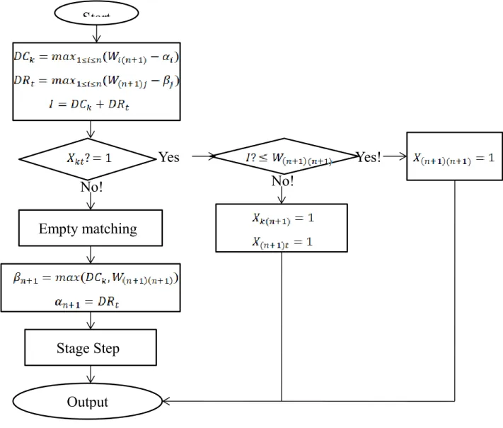
Figure 24: The overall program flow chart ... 49

Figure 25: 𝟑 × 𝟑 matrix ... 52

Figure 26: 4×4 matrix ... 52

Figure 27: 4×4 matrix ... 53

Figure 28: 𝟒 × 𝟒 matrix ... 53

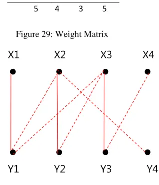
Figure 29: Weight Matrix ... 54

Figure 30: Equality subgraph ... 54

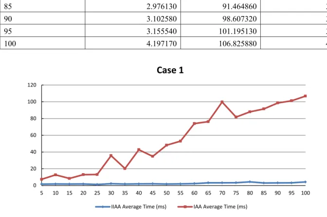
Figure 31: Trend lines for average operation time for different dimensions ... 56

Figure 32: Trend lines for operation time for different dimensions ... 58

Figure 33：Chances and the percentage of general cases ... 60

Figure 34：A clinic with 20 nurses and 4 departments ... 65

Figure 35: Evaluation values of agents and roles and the assignment matrix ... 66

Figure 36: A clinic adding a new department ... 67

(11)

xi

Figure 38: Optimal solution ... 68

Figure 39: A new nurse joins the clinic ... 69

Figure 40: Evaluation values of nurses and departments and the assignment matrix ... 69

Figure 42: A new department and a new nurse join the clinic... 71

Figure 43: Evaluation values of nurses and departments and the assignment matrix ... 71

Figure 45: Matrix with optimal solution ... 74

Figure 46: Matrix extended with a new column, 𝑳 = [𝟏, 𝟐, 𝟏, 𝟏] ... 75

Figure 47: Matrix after subtracting ... 75

Figure 48: Matrix extended with a new column, 𝑳 = [𝟏, 𝟐, 𝟏, 𝟐] ... 76

Figure 49: Matrix after subtracting ... 76

Figure 50: Matrix extended with a new column, 𝑳 = [𝟏, 𝟐, 𝟏] ... 77

Figure 52: Matrix extended with a new column, 𝑳 = [𝟏, 𝟐, 𝟏] ... 78

Figure 54: Matrix extended with a new column, 𝑳 = [𝟏, 𝟐, 𝟏, 𝟏] ... 79

Figure 56: Matrix with optimal solution (𝑳 = [𝟏, 𝟏, 𝟏, 𝟏]) ... 80

(12)

xii

Figure 58: Optimal solution ... 81 Figure 59: Matrix extended with a new column, 𝑳 = [𝟏, 𝟏, 𝟏, 𝟐, 𝟏] ... 82 Figure 60: Matrix extended with a new column, 𝑳 = [𝟏, 𝟏, 𝟏, 𝟐, 𝟏] ... 83

(13)

xiii

List of Appendix

Appendix I ... 93 Appendix II ... 94 Appendix III ... 95

(14)

xiv

Abbreviations

GRAP Group Role Assignment Problem RBC Role-Based Collaboration

GAP Generalized Assignment Problem AP Assignment Problem

IAP Incremental Assignment Problem IAA Incremental Assignment Algorithm

IIAA Improved Incremental Assignment Algorithm IGRAP Improved Group Role Assignment Problem

(15)

Chapter 1 Assignment Problem

1

This chapter is a review of the Assignment Problem (AP) and its algorithms. This chapter includes:

 The introduction of AP  Perfect matching

 Bipartite matching algorithm  Linear Assignment Problem

(16)

1.1 Background

In recent years, there are many situations concerning assignment arise in many fields, such as, medical institution, business, transportation, education fields, and sports. The

assignment problem is under optimization or operations research branches. It is a widely studied topic in combinatorial optimization problems [1]. In addition, the assignment problem is an important subject for solving many problems around the world [2].

Assignment problems are to assign 𝑛 items to 𝑛 other items [3] in an optimal way. The two components are the objective function and the assignments. The objective function reflects the expectation of optimizing as much as possible, while the assignment represents the

underlying combinatorial structure. The problem is to minimize the total costs of operating the tasks or maximize the total profit of allocation. A table or matrix can be shown as assignment problem. Generally, the rows represent people or objects to assign, the columns stand for the tasks or things to be assigned [1].

A bipartite graph can be used to describe assignments. The definition of the bipartite graph is: A graph 𝐺 = (𝑈, 𝑉; 𝐸) has two vertex sets 𝑈 and 𝑉 which are not disjoint. 𝐸 is an edge set. If every edge connects a vertex of 𝑉 and there are no edges which have both endpoints in 𝑈 and 𝑉, then 𝐺 is called bipartite. A subset of the edges such that every vertex of 𝐺 meets at most one edge of the matching is called a matching 𝑀 in 𝐺. Suppose that the number of vertices in 𝑈 and 𝑉 equals 𝑛, i.e., |𝑈| = |𝑉| = 𝑛. If in this case, the matching 𝑀 is called a perfect matching when each vertex of 𝐺 coincides with an edge of the matching 𝑀. Obviously, every assignment can be shown as a perfect matching [4], shown in Figure 1.

(17)

Figure 1: Representation of assignment

Given a bipartite graph 𝐺 = (𝑈, 𝑉; 𝐸) and its edge set 𝐸 and two vertex sets 𝑈 and 𝑉 which are not disjoined. The assignment problem is to find a set of 𝑛 edges in the bipartite graph such that every vertex coincides with exactly one edge. It is also known as the Bipartite Perfect Matching Problem.

1.2 Perfect Matching

We will discuss whether there exists an assignment (i.e., a perfect matching) in a given bipartite graph or not in this section. Hall’s Marriage Theorem gives a basic answer to this question in 1935 [5]. There is a necessary and sufficient condition is stated which is known as the Hall’s Marriage Theorem for finding the perfect matching in a bipartite graph. For a vertex

𝑖/𝑈, let 𝑁(𝑖) denote the set of its neighbors, i.e., the set of all vertices 𝑗/𝑉 which are connected with 𝑖 by an edge in 𝐸. When we consider the vertices in 𝑈 as young men and the vertices in 𝑉 as young ladies, the set 𝑁(𝑖) contains the friends of 𝑖. Moreover, for any subset 𝑈 of 𝑈 let

𝑁(𝑈) = ⋃𝑖∈𝑈𝑁(𝑖). The Theorem 1.2.1, 1.2.2 and 1.2.3 are presented by Hall [5].

Theorem 1.2.1. (Hall [5]F, 1935.)Let 𝐺 = (𝑈, 𝑉; 𝐸) be a bipartite graph. It is possible to match every vertex of 𝑈 with a vertex of 𝑉 if and only if for all subsets 𝑈 of 𝑈

|𝑈| ≤ |𝑁(𝑈)| (Hall’s condition)

Theorem 1.2.2.(Marriage theorem.)Let 𝐺 = (𝑈, 𝑉; 𝐸) be a bipartite graph with

|𝑈| = |𝑉|. There exists a perfect matching (marriage) in 𝐺 if and only if 𝐺 fulfills Hall’s condition.

(18)

Theorem 1.2.3.(K𝐨̈nig’s matching theorem [19], 1931.) In a bipartite graph the minimum number of vertices in a vertex cover equals the maximum cardinality of a matching:

𝑚𝑖𝑛

𝐶 𝑣𝑒𝑟𝑡𝑒𝑥 𝑐𝑜𝑣𝑒𝑟|𝐶| =𝑀 𝑚𝑎𝑡𝑐ℎ𝑖𝑛𝑔𝑚𝑎𝑥 |𝑀| .

1.3 Bipartite Matching Algorithms

In assignment problems, it is an important subject to finding a maximum matching in a bipartite graph.

1.3.1 A labeling (dual variables) method to find a maximum matching

Given a bipartite graph 𝐺 = (𝑈, 𝑉; 𝐸) and a matching 𝑀 (𝑀 might even be empty). If an edge of 𝐸 belongs to 𝑀, it is called a matching edge, if not a non-matching edge. Edges are alternately matching and non-matching is called an Alternating Path. An Augmenting Path 𝑃 is an Alternating Path that starts from a free (unmatched) vertex and ends on a free (unmatched) vertex.

bipartite graph alternating/ augmenting path

Figure 2: Bipartite graph & alternating/ augmenting graph

In Figure 2, let 𝑀 be a matching of G. Vertex 𝑣 is matched if it is the endpoint of an edge in 𝑀; otherwise 𝑣 is free. 𝑌₂, 𝑌₃, 𝑌₄, 𝑌₆, 𝑋₂, 𝑋₄, 𝑋₅, 𝑋₆ are matched, other vertices are free.

𝑌₅, 𝑋₆, 𝑌₆ is an alternating path. 𝑌₁, 𝑋₂, 𝑌₂, 𝑋₄, 𝑌₄, 𝑋₅, 𝑌₃, 𝑋₃ is an augmenting path. Y1 Y2 Y3 X1 X2 X3 Y4 Y5 Y6 X4 X5 X6 Y1 Y2 Y3 X1 X2 X3 Y4 Y5 Y6 X4 X5 X6

(19)

The definition of augmentation: Let 𝑃 be an augmenting path with respect to the matching 𝑀. There are two rules that the matching augmented by 𝑃 is obtained [4].

The first rule is the unmatched and matching edges in 𝑃 change their roles (all previously matching edges of 𝑀 ∩ 𝑃 become unmatched edges, at the same time, all previously unmatched edges of 𝑀 ∩ 𝑃 now become matching). The second rule is all matching edges of 𝑀 which do not lie on the path 𝑃 remain to be the matching edges.

If 𝑀 is not a maximum matching in 𝐺, then there exists an augmenting path 𝑃 with respect to 𝑀, and 𝑀 = 𝑀 ∈ 𝑃 is a matching in 𝐺 with |𝑀| = |𝑀| + 1 [7]. The cardinality matching algorithm is presented below [4]:

Cardinality matching algorithm:

𝑀 is a matching in graph 𝐺 = (𝑈, 𝑉; 𝐸) (possibly 𝑀 = ∅);

𝐿 contain all unmatched vertices of 𝑈;

Labeled vertices on the right side are collected in the set 𝑅;

𝑅 ∶= ∅;

while 𝐿 ∪ 𝑅 ≠ ∅do

choose a vertex 𝑥 from 𝐿 ∪ 𝑅;

if𝑥/𝐿then Scan_leftvertex(𝑥)else Scan_rightvertex(𝑥)

endwhile

Procedure Scan_leftvertex(𝑥)

𝐿 ∶= 𝐿 \ {𝑥};

(20)

label 𝑗 as 𝑙(𝑗) ∶= 𝑥;

𝑅 ∶= 𝑅 ∪ {𝑗} endwhile

Procedure Scan_rightvertex(𝑥)

𝑅 ∶= 𝑅 \ {𝑥};

if there is a matching edge[𝑖, 𝑥]then

label 𝑖 as 𝑟(𝑖) ∶= 𝑥;

𝐿 ∶= 𝐿 ∪ {𝑖}

else [comment: augmentation of the matching]

starting from 𝑥, find the alternating path 𝑃 by backtracking the labels;

𝑃 ∶= (… , 𝑟(𝑙(𝑥)), 𝑙(𝑥), 𝑥);

𝑀 ∶= 𝑀 ∈ 𝑃;

let 𝐿 contain all unmatched vertices of 𝑈;

𝑅 ∶= ∅;

cancel all labels

endif

The algorithm starts with an matching 𝑀 which is arbitrary. The matching 𝑀 gradually increases (augments) this matching step-by-step by way of augmenting paths until a maximum matching is reached. At each augmentation, one additional vertex of 𝑈 is matched. Therefore, there will be at most 𝑛 augmentations. In addition, every vertex is labeled no more than once for

(21)

each augmentation. Therefore, finding a augmenting path requires at most 𝑂(𝑚) steps, the operation time is 𝑂(𝑛𝑚).

1.3.2 Other Algorithms

Hopcroft and Karp [6] propose an algorithm that not only augments the augmentation by augmenting path, but also augments the matching by the largest disjoint aurmenting path system with the same minimum length. It runs in 𝑂(𝑚√𝑛) time.

Alt, Blum, Mehlhorn, and Paul [8] do some improvement on Hopcroft and Karp’s method for the case of “dense” graphs by using a fast adjacency matrix scanning technique of Cheriyan, Hagerup and Mehlhorn [9]. Therefore they get an algorithm that improves the running time in 𝑂(𝑛1.5√𝑚 log 𝑛⁄ ) to find the maximum bipartite matching, where 𝑛 = |𝑈| + |𝑉|, where

𝑈 and 𝑉 are vertex sets.

The rank of matrices has a close relationship with maximum matching. Another

stochastic method is based on the algorithm which is called fast matrix multiplication and gives complexity of 𝑂(𝑛2.376) [10]. It is theoretically better for sufficiently dense graphs, but the algorithm is slower in practice.

1.3.3 Applications of the Maximum Matching Algorithm

(1) Vehicle scheduling problems

When planning the operative public transport, the vehicle scheduling problem (VSP) is one of the most important tasks [11]. The set of schedule trips is given that the travel (departure and arrival) time is fixed, as well as the start and end locations, and travel times between all pairs of end stations, the aim is to find the assignment of trips to the vehicles in order to accurately cover each trip once, each vehicle performs a feasible itinerary sequence of trips [12].

(22)

(a) (b)

Figure 3: (a) the network which cover all nodes with a minimum number of node disjoint paths (the bold line is shown the network); (b) shows the corresponding maximum matching [4].

A disjoint path problem modeled as this problem in a network. An example is shown in Figure 3(a). Then convert it to a maximum matching problem in a bipartite graph. Figure 3(b) shows the connect lines between the node disjoint paths of Figure 3(a) and matching.

(2) Time slot assignment problem

When using satellites in telecommunication systems, the data first to be remitted are first buffered in the ground station, then the data are transmitted to the satellite in very short data bursts, they are amplified and send back to Earth. The Time Division Multiple Access (TDMA)

a

b

c

d

e

f

g

h

a

b

c

d

e

f

g

h

a

b

c

d

e

f

g

h

(23)

technique can be used. A transponder connects the receiving station to the sending station. The time slot assignment problem solves the problem of which switching modes should be applied. It also figures out how long each of them lasts in a given amount of data can be remitted in the shortest possible time [13]. The time complexity is 𝑂(𝑛4₎_.

1.4 Linear Assignment Problem

The general purpose of the assignment problem is to optimize the resources distribution. Resources demand points, and both resources and demand point have the same number [2]. Mathematically, the Linear Assignment Problem can be proposed following:

∑𝑛𝑖=1∑𝑛𝑗=1𝑐𝑖𝑗𝑥𝑖𝑗 (1.4.1) subject to ∑𝑛 𝑥_𝑖𝑗 = 1 𝑗=1 , 𝑖 = 1,…,𝑛 (1.4.2) ∑𝑛 𝑥_𝑖𝑗 = 1 𝑖=1 , 𝑗 = 1,…,𝑛 (1.4.3) 𝑥_𝑖𝑗 = 0 or 1, 𝑖 = 1 ,…,𝑛, 𝑗 = 1,…,𝑛 (1.4.4)

Where 𝑐_𝑖𝑗 is the cost of effectiveness when assigning 𝑖th resource to 𝑗th demand, 𝑥_𝑖𝑗 is 0 or 1 (as presented in (1.4.4)), and 𝑛 is the number of resources or demands. The constraints of the assignment problem are defined as (1.4.2) - (1.4.4). Equation (1.4.22) indicates that each resource 𝑖 only can be assigned to one demand 𝑗, while (1.4.3) shows that each demand 𝑗 only can be assigned to one resource 𝑖.

However, this theorem is not directly an efficient method for finding a perfect matching. In the early days of mathematical programming, labeling methods were used to create a perfect matching of the 𝑂(𝑛3) complexity. Several authors improved on these methods later. One of the well-known methods is Hopcroft and Karp [6], which show that a perfect matching can be found in 𝑂(𝑛5 2⁄ ) times. We will present this algorithm below.

Regarding every assignment problem, there is a matrix called cost or validity matrix

(24)

assignment matrix, where each resource can only be assigned to a requirement and represent it, as given in the following:

( 𝑐₁₁ 𝑐₂₁ ⋮ 𝑐𝑛1 𝑐₁₂ 𝑐₂₂ ⋮ 𝑐𝑛2 𝑐₁₃ 𝑐₂₃ ⋮ 𝑐𝑛3 ⋯ ⋯ ⋮ ⋯ 𝑐_1𝑛 𝑐_2𝑛 ⋮ 𝑐𝑛𝑛 ) (1.4.5)

Which is always a square matrix.

Here is a real world scenario. Assume that 𝑛 jobs are to be assigned to 𝑛 machines (or workers) in the best possible way. Let us assume that machine 𝑗 needs 𝑐𝑖𝑗 time units to process job 𝑖. We want to minimize the total completion time. If we assume that the machines work in series, we must minimize the linear sum objective function. If we assume that the machines work in parallel, we have to minimize the bottleneck objective function.

This example shows different objective functions of interest. When it is necessary to minimize cost, the sum objective is usually used. If a time need to be minimized, a so-called bottleneck objective function is often used. Although this function is not written in linear form, the optimization problem with this objective function is called “linear” compared to the quadratic problems introduced in Section 1.5.

1.4.1 Linear Sum Assignment Problem

The most well-known problems in linear programming and in combinatorial optimization is the linear sum assignment problem (LSAP). Informally, we are given an 𝑛 × 𝑛 cost matrix

𝐶 = (𝑐_𝑖𝑗) and we want to match each row to a different column in order to minimize the sum of the corresponding entries. In other words, we want to select 𝑛 elements of 𝐶 so that there is only one element in each row and one in each column and the sum of the corresponding costs is a minimum.

Alternatively, LSAP can be defined through a graph theory model, for example, a bipartite graph 𝐺 = (𝑈, 𝑉; 𝐸) having a vertex of 𝑈 for each row, a vertex of 𝑉 for each column, and cost 𝑐𝑖𝑗 associated with edge [𝑖, 𝑗](𝑖, 𝑗 = 1,2, … 𝑛). The problem is then to determine the minimum cost perfect matching in 𝐺 (weighted bipartite matching problem: find a subset of

(25)

edges so that each vertex happens to belongs to exactly one edge and the sum of the costs of these edges is a minimum).

They mainly occur in sub-problems in more complex cases, such as the travelling salesman problems, vehicle routing problems, personnel assignments and similar problems in practice [3]. Neng [14] describes an interesting application in railway systems. He considers the problem of assigning engines to trains due to traffic restrictions and expressed this problem as a linear assignment problem.

A large number of sequential and parallel algorithms has been developed for the LSAP, such as primal-dual algorithms, simplex-like methods, cost operation algorithms, forest

algorithms and relaxation approaches. For a survey on these methods and available computer programs see the recent article of Burkard and Çela [15] or the annotated bibliography of Dell’ Amico and Martello [16]. Nowadays it is possible to solve large scale dense LSAPs (with

𝑛 ≈ 106_{) within a couple of minutes, see [17].}

Although 𝑂(𝑛3) is the best worst case complexity for sequential linear sum assignment algorithms, Karp [18] develope an algorithm with the expected running time of 𝑂(𝑛2 log 𝑛) in the case of independent and uniformly distributed cost coefficients 𝑐𝑖𝑗 in [0, 1].This algorithm is a special implementation of the classical shortest augmenting path algorithm. It uses priority queues to compute shortest augmenting paths in 𝑂(𝑛2 log 𝑛) time which produces a worst case time complexity of 𝑂(𝑛3 log 𝑛).

1.4.1.1 Mathematical Model

The linear sum assignment problem (LSAP) can be stated as

min ∑𝑛𝑖=1∑𝑛𝑗=1𝑐𝑖𝑗𝑥𝑖𝑗 (1.4.1.1.1) subject to ∑𝑛 𝑥_𝑖𝑗 = 1 𝑗=1 , 𝑖 = 1,…,𝑛 ∑𝑛𝑖=1𝑥𝑖𝑗 = 1, 𝑗 = 1,…,𝑛

(26)

𝑥𝑖𝑗 = 0 or 1, 𝑖 = 1 ,…,𝑛, 𝑗 = 1,…,𝑛

By associating dual variables 𝑢_𝑖 and 𝑣_𝑗 with assignment constraints (1.4.1.1.2) and (1.4.1.1.3), respectively, the dual problem is

max ∑𝑛_𝑖=1𝑢_𝑖 + ∑𝑛_𝑗=1𝑣_𝑗 (1.4.1.1.2)

s.t. 𝑢𝑖 + 𝑣𝑗 ≤ 𝑐𝑖𝑗 (𝑖, 𝑗 = 1,2, … 𝑛) (1.4.1.1.3) By duality theory, a pair of solutions respectively feasible for the primal and the dual is optimal if and only if

𝑥_𝑖𝑗(𝑐_𝑖𝑗 − 𝑢_𝑖 − 𝑣_𝑗) = 0(𝑖, 𝑗 = 1,2, … 𝑛) (1.4.1.1.4)

1.4.1.2 An

𝑂(𝑛

4

)

implementation of the Hungarian Algorithm

The Hungarian algorithm is considered to be a predecessor of the primal-dual method for linear programming. It begins with a feasible dual solution 𝑢, 𝑣 satisfying (1.4.1.1.3) and a partial primal solution (in which less than 𝑛 rows are assigned) satisfying the condition

(1.4.1.1.4) with respect to 𝑢, 𝑣. Each iteration solves a restricted primal problem independent of the costs, attempting to increase the cardinality of the current assignment by operating on the partial graph of 𝐺 = (𝑈, 𝑉; 𝐸) that only contains the edges of 𝐸 having zero reduced costs. If the attempt is successful, a new primal solution in which one more row is assigned is obtained. Otherwise, updating the current dual solution to get a new edge with zero reduction.

The main idea of the method is as follows: consider we only use the edge of weight 0 (called the “0-weight edges”) to find the perfect matching. Obviously, these edges will be the solution of the assignment problem. If we cannot find perfect matching on the current step, then the Hungarian algorithm changes weights of the available edges so that the new 0-weight edges appear and these changes do not affect the optimal solution [38].

Preliminaries. For each vertex from the left part, find the minimal outgoing edge and subtract its weight from all weights of the connection to the vertex. This will introduce 0-weight edges (at least one). Apply the same procedure for the vertices in the right part.

(27)

Figure 4: The preliminaries [38]

u

₃

u

₂

v

₁

(28)

Step 2. Let ∆= 𝑚𝑖𝑛_{𝑖∉𝑈,𝑗∉𝑉}(𝑐_𝑖𝑗) and adjust the weights by using the rule as follows: 𝑐_𝑖𝑗 = { 𝑐_𝑖𝑗 − ∆, 𝑖 ∉ 𝑈˄𝑗 ∉ 𝑉 𝑐_𝑖𝑗, 𝑖 ∈ 𝑈˅𝑗 ∈ 𝑉 𝑐_𝑖𝑗+ ∆, 𝑖 ∈ 𝑈˄𝑗 ∈ 𝑉 (a) (b)

Figure 6: (a) Graph with modified weights (delta=1); (b) Minimum matching [38].

Step 3. Repeat Step 1 until solved.

In this example, we are using the Hungarian Algorithm to solve the minimum value of the matrix. The perfect matching is (𝑢1, 𝑣2), (𝑢2, 𝑣3), (𝑢3, 𝑣1) which is 4+6+5=15.

₁

(29)

1.4.1.3 An

𝑂(𝑛

3

)

implementation of the Hungarian Algorithm

We will introduce the maximum-weighted matching problem in this section. Obviously, it is easy to transform minimum problem to the maximum one, just by setting:

𝑤(𝑢, 𝑣) = −𝑤(𝑢, 𝑣), ∀(𝑢, 𝑣) ∈ 𝐸

or 𝑤(𝑢, 𝑣) = 𝑀 − 𝑤(𝑢, 𝑣), 𝑀 = max_{(𝑢,𝑣)∈𝐸}𝑤(𝑢, 𝑣)

Given a matching 𝑀, a path is alternating that begins with an unmatched vertex and whose edges belong alternately to the matching and not to the matching. It is called an

alternating path. An augmenting path is an alternating path that starts from and ends on free (unmatched) vertices. All alternating paths originating from a given unmatched node form a Hungarian tree.

The algorithm assigns dual variables 𝛼_𝑖 and 𝛽_𝑗 to each node 𝑈 and node 𝑉 respectively. The assignment problem is feasible when 𝛼_𝑖+ 𝛽_𝑗 ≥ 𝑊_𝑖𝑗. The Hungarian algorithm maintains feasible values for all the 𝛼𝑖 and 𝛽𝑗 from initialization to termination. When 𝛼𝑖+ 𝛽𝑗 = 𝑊𝑖𝑗, an edge in the bipartite graph is called admissible. The sub-graph containing only the currently admissible edges is called the equality sub-graph 𝐺’.

Starting from an empty matching, the basic strategy adopted by the Hungarian algorithm is to repeatedly search for augmenting paths in the equality sub-graph. If an augmenting path is found, the current match set is augmented by flipping the matched and unmatched edges along this path. Because there is one more unmatched than matched edge, this flipping increases the cardinality of the matching by one, completing a single stage of the algorithm. If an augmenting path is not found, adjust the dual variables to bring extra edges into the equality sub-graph by making them admissible and the continue searching. These stages of the algorithm are executed to determine 𝑛 matches, at which point the algorithm terminates [19].

An outline of the Hungarian algorithm for the assignment problem is shown below [19].

Hungarian Algorithm:

(30)

weights 𝑊_𝑖𝑗

Output: A complete matching, 𝑀

1. Perform initialization:

(a) Begin with an empty matching, 𝑀 = ∅

(b) Assign feasible values to the dual variables 𝛼_𝑖 and 𝛽_𝑗 as follows:

∀𝑢𝑖 ∈ 𝑈, 𝛼𝑖 = 0 (1.4.1.3.1) ∀𝑣𝑗 ∈ 𝑉, 𝛽𝑗 = 𝑚𝑎𝑥𝑖𝑊𝑖𝑗 (1.4.1.3.2) 2. Perform 𝑛 stages of the algorithm, each given by the routine Stage.

3. Output the matching after the 𝑛𝑡ℎ stage: 𝑀 = 𝑀𝑛.

Stage:

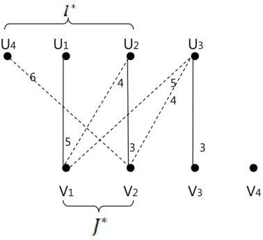
1. Designate each exposed (unmatched) node in 𝑈 as the root of a Hungarian tree. 2. Grow the Hungarian tree rooted at the exposed nodes in the equality sub-graph.

Designate the indices 𝑖 of nodes 𝑢_𝑖 encountered in the Hungarian tree by the set 𝐼∗_{, and the} indices 𝑗 of nodes 𝑣_𝑗 encountered in the Hungarian tee by the set 𝐽∗_{. If an augmenting path} is found, go to Step 4. If not, and the Hungarian trees cannot be grown further, proceed to

Step 3.

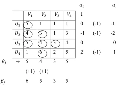
3. Modify the dual variables 𝛼_𝑖 and 𝛽_𝑗 as follows to add new edges to the equality subgraph.

Then go to Step 2 to continue the search for the augmenting path.

𝜃 = 𝑚𝑖𝑛 𝑖∈𝐼∗_,𝑗∉𝐽∗(𝛼𝑖+ 𝛽𝑗− 𝑊𝑖𝑗) 𝛼_𝑖 ← {𝛼_𝛼𝑖 − 𝜃 𝑖 ∈ 𝐼∗ 𝑖 𝑖 ∉ 𝐼∗ 𝛽_𝑗 ← {𝛽𝑗+ 𝜃 𝑗 ∈ 𝐽 ∗ 𝛽_𝑗 𝑗 ∉ 𝐽∗

4. Augment the current matching by flipping matched and unmatched edges along the

selected augmenting path. That is, 𝑀_𝑘 (the new matching at stage 𝑘) is given by (𝑀_𝑘−1− 𝑃) ∪ (𝑃 − 𝑀𝑘−1), where 𝑀𝑘−1 is the matching from the previous stage and 𝑃 is the set of edges on the selected augmenting path.

(31)

Example: Consider the 3 × 3 weighted bipartite graph described by its weight matrix in the following: 𝑣₁ 𝑣₂ 𝑣₃ 𝑢1 1 4 5 𝑢₂ 5 7 6 𝑢3 5 8 8 Figure 7: 𝟑 × 𝟑 matrix

Initialing the graph, trivial labeling and associated equality graph.

(a) (b)

Figure 8: (a) Original graph; (b) Equality subgraph+Matching.

The Hungarian tree can be grown rooted at the nodes 𝑢₁ in the equality subgraph.

𝐼∗ _{= {𝑢}

1} and 𝐽∗ = ∅. 𝑀 = {(𝑢2, 𝑣1), (𝑢3, 𝑣2), (𝑢3, 𝑣3)}. The augmenting path cannot be found.

𝜃 = 𝑚𝑖𝑛_𝑖∈𝐼∗_,𝑗∉𝐽∗{

0 + 5 − 1 (𝑢1, 𝑣1) 0 + 8 − 4 (𝑢1, 𝑣2) 0 + 8 − 5 (𝑢₁, 𝑣₃)

=3

Reduce labels of 𝐼∗ by 3. 𝐼∗ = {𝑢₁} and 𝐽∗ = {𝑣₃}. Then we got the new equality subgraph and the augmenting path 𝑢₁, 𝑣₃, 𝑢₃, 𝑣₂. Flipping matched to augment the current

v₁ v₂ v₃ u₁ u₂ u₃ 1 4 5 5 7 6 5 8 8 5 8 8 0 0 0 u₁ 0 u₂ 0 u₃ 0 5 8 8 v₁ 5 v₂ 8 v₃ 8

(32)

matching and unmatched edges along the selected augmenting path.

Mk= {(𝑢2, 𝑣1), (𝑢3, 𝑣2), (𝑢1, 𝑣3)}.

(a) (b)

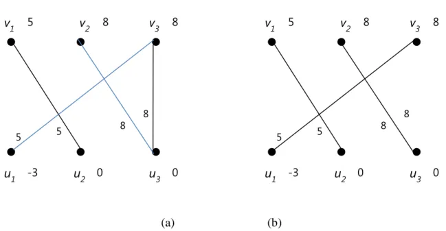
Figure 9: (a) New equality subgraph; (b) Matching.

In each iteration, we increment matching. Therefore, we have 𝑛 iterations [4]. At each iteration, each edge of the graph is used no more than once when finding augmenting path, so we've got 𝑂(𝑛2) complexity. Concerning labeling we update slack array each time when we insert vertex from 𝑈 into 𝐼∗, so each iteration does not occur more than 𝑛 times, updating slack takes 𝑂(𝑛) operations, so again we've got 𝑂(𝑛2). Updating labels occur no more than 𝑛 times per iterations (since we add at least one vertex from 𝑉 to 𝐽∗ on each iteration), it takes 𝑂(𝑛) operations. Therefore the total complexity of this implementation is 𝑂(𝑛3).

Jonker and Volgenant [20] develope an improved 𝑂(𝑛3) Hungarian algorithm. Fortran implementations of Hungarian algorithm are proposed by McGinnis [21], Carpaneto and Toth [22], and Carpaneto, Martello, and Toth [23]. The Carpaneto and Toth [22] paper, which includes the Fortran listing of their code, provides computational comparisons with the primal simplex algorithm by Barr, Glover, and Klingman [24].

u₁ -3 u₂ 0 u₃ 0 5 8 8 v₁ 5 v₂ 8 v₃ 8 5 u₁ -3 u₂ 0 u₃ 0 5 8 8 v₁ 5 v₂ 8 v₃ 8 5

(33)

1.4.1.4 Other algorithms

Dinic and Kronrod [25] has proposed a different approach that is completely independent of the linear programming duality theory.

The most efficient LSAP algorithm is based on shortest augmenting path techniques. In the early 1960s, Hoffman and Markowitz [26] observe that an LSAP can be solved through a sequence of 𝑛 shortest paths on cost matrices of increasing size from 1 × 1 to 𝑛 × 𝑛. However such matrices can include negative costs, so each shortest path search would require 𝑂(𝑛3) time. In early 1970s Tomizawa [27] and Edmonds and Karp [28] study shortest path algorithms for the min-cost flow problem observe that by using the reduced costs, Dijkstra algorithm can be applied to obtain an 𝑂(𝑛3) time algorithm for LSAP.

Dantzig [29] specialize the primal simplex algorithm into a network problem, which is the starting point for all primal simplex-based algorithms for LSAP. Gavish, Schweitzer and Shlifer [30] give computational results on the effect of various pivoting rules on the number of degenerate pivots in the solution of LSAP. In general, the primal algorithms are less efficient than other methods.

1.4.2 The Linear Bottleneck Assignment Problem

Fulkerson, Gllicksberg, and Gross [31] introduce the problem of linear bottleneck assignment. It happens when a job is assigned to a parallel machine to minimize the latest completion time. Another application is to locate objects in space. Let 𝑛 jobs and 𝑛 machines be given. The cost coefficient 𝑐𝑖𝑗 is the time required for machine 𝑗 to complete job 𝑖. If the

machines work in parallel and we want to assign the jobs to the machines such that the latest completion time is as early as possible, it can mathematically be written as

min max ∑𝑛_𝑖=1∑𝑛_𝑗=1𝑐_𝑖𝑗𝑥_𝑖𝑗 (1.4.2.1)

subject to

∑𝑛 𝑥_𝑖𝑗 = 1

𝑗=1 , 𝑖 = 1,…,𝑛 ∑𝑛𝑖=1𝑥𝑖𝑗 = 1, 𝑗 = 1,…,𝑛

(34)

𝑥𝑖𝑗 = 0 or 1, 𝑖 = 1 ,…,𝑛, 𝑗 = 1,…,𝑛

Solving an LBAP with cost matrix 𝐶 = (𝑐_𝑖𝑗) can produce very good results in practice. A similar technique can be used to track missiles in space. If their locations at two different times

𝑡₁ and 𝑡₂ are known, the squared Euclidean distances between any pair of old and new locations are calculated and the corresponding linear bottleneck assignment problem is solved to match the points in the right way.

1.4.3

1.5

1.5.1 Quadratic Assignment problems

The quadratic assignment problem (QAP) is introduced by Koopmans and Beckmann [35] in 1957 as a mathematical model for the location of indivisible economical activities. A set of 𝑛 facilities has to be allocated to a set of 𝑛 locations. We give three 𝑛 × 𝑛 input matrices:

(35)

𝐴 = (𝑎𝑖𝑘), 𝐵 = (𝑏𝑗𝑙), and 𝐶 = (𝑐𝑖𝑗), where 𝑎𝑖𝑘 is the flow between facility 𝑖 and facility 𝑘, 𝑏𝑗𝑙 is the distance between location 𝑗 and location 𝑙, and 𝑐_𝑖𝑗 is the cost of placing facility 𝑖 at location 𝑗. We assume that the total cost depends on the flow between facilities multiplied by their distance and the cost for placing a facility at a certain site. The goal is to assign each facility to a location to minimize the total cost.

The quadratic assignment problem can be modeled as:

min∑𝑖=1𝑛 ∑𝑗=1𝑛 ∑𝑛𝑘=1∑𝑛𝑙=1𝑎𝑖𝑘𝑏𝑗𝑙𝑥𝑖𝑗𝑥𝑘𝑙+ ∑𝑖=1𝑛 ∑𝑛𝑗=1𝑐𝑖𝑗𝑥𝑖𝑗 (1.5.1.1) subject to ∑𝑛 𝑥_𝑖𝑗 = 1 𝑗=1 , 𝑖 = 1,…,𝑛 ∑𝑛 𝑥_𝑖𝑗 = 1 𝑖=1 , 𝑗 = 1,…,𝑛 𝑥_𝑖𝑗 = 0 or 1, 𝑖 = 1 ,…,𝑛, 𝑗 = 1,…,𝑛

Quadratic assignment problems are so-called 𝑁𝑃-hard problems. This means that an optimal solution can only be found by enumeration of all possibilities unless 𝑃 = 𝑁𝑃.

1.5.2 Multi-index Assignment problems

In 1968, Pierskalla [36] introduces Multi-index assignment problems as a natural

extension of linear assignment problems. For a long time only 3-index assignment problems have been considered, and in recent years, more than 3 indices problems have been investigated, mainly in the context of multi-target tracking and data association problems [37].

(36)

Chapter 2 Group Role Assignment Problem

2

This chapter is a review of the Group Role Assignment Problem (GRAP). Generalized Assignment Problem (GAP) is related to GRAP, this chapter presents:

 The introduction of GRAP,  The introduction of GAP,

 The mathematical formulation of the GAP,  Literature review of the GAP,

 Role-Based Collaboration,

 The mathematical formulation of the GRAP, and  The solution of GRAP

(37)

2.1 Introduction

In the real world, different people can be involved in different roles in different fields, such as sports players, doctors, teachers, etc. Roles are commonly concepts in many fields, e.g., behavioral science, sociology, drama, social psychology, management and psychology [39]. Therefore, collaboration is necessary to get the optimal performance of the entire system. Role-Based Collaboration (RBC) is a method to promote an organizational structure, to provide ordered system behavior, and to integrate system security for both human and nonhuman entities that collaborate and coordinate their activities within systems [40]. Take a soccer team as an example; every football player has different performance when assigned to each role. How to assign football players to different roles and get their best performances in that role is the ultimate purpose for the coach. In order to solve these kinds of problems, RBC is a useful and functional methodology.

In RBC, role assignment is a crucial task that affects the collaboration efficiency and the level of satisfaction of all the participating members involved in. It can be divided into three steps: agent evaluation, group role assignment, and role transfer [40]. Group role assignment problem (GRAP) initiates a group by assigning roles to its members or agents to achieve its highest performance. Considering the same example above, in a soccer team, if a coach wants to pick up 11 football players from 20 players for four roles: one goalkeeper, four backs, three midfields, and three forwards, how to make role assignment to optimize the whole team’s performance is a typical GRAP.

GRAP can be transferred to the Generalized Assignment Problem (GAP). The well-known Kuhn-Munkres (K-M) algorithm is designed to solve the GAP with the complexity of

𝑂(𝑛3₎_{, GRAP can be solved efficiently.}

The objective of GAP is to find an assignment in which all agents minimize their costs or the total profit of the assignment is maximized. The GAP has been given the optimal or

(38)

2.2 Generalized Assignment Problem

The generalized assignment problem (GAP) is a problem in combinatorial optimization. When the number of tasks and agents are equal, it is known as a generalization form of a

classical Assignment Problem (AP). This means that for GAP, the number of agents assigned to each task could be different.

The goal of GAP is to find an assignment in which all agents minimize their costs or maximize the total profit. It has been applied to many applications, such as various routing problems and flexible manufacturing systems [41].

2.2.1 The Mathematical Formulation of the GAP

Given 𝑛 jobs (𝑗 = 1, … 𝑛) and 𝑚 agents (𝑖 = 1, … , 𝑚), each job should be assigned to only one agent to maximize the total profit without exceeding their budget.

GAP can be formulated as an integer programming problem

{ 𝑚𝑎𝑥 ∑ ∑ 𝑝_𝑖𝑗𝑥_𝑖𝑗 𝑛 𝑗=1 𝑚 𝑖=1 (2.2.1) 𝑠. 𝑡. ∑ 𝑤_𝑖𝑗𝑥_𝑖𝑗 ≤ 𝑐_𝑖 𝑛 𝑗=1 𝑖 = 1, … , 𝑚; (2.2.2) ∑ 𝑥𝑖𝑗 𝑚 𝑖=1 = 1 𝑗 = 1, … , 𝑛; (2.2.3) 𝑥𝑖𝑗 ∈ {0,1} 𝑖 = 1, … , 𝑚, 𝑗 = 1, … , 𝑛; (2.2.4) where

𝑥_𝑖𝑗 = {1 if job 𝑗 is assigned to agent 𝑖 0 otherwize

The parameters can be defined as follows: the profit of assigning job 𝑗 to agent 𝑖 is represented by 𝑝_𝑖𝑗, the weight of assigning job 𝑗 to agent 𝑖 is represented by 𝑤_𝑖𝑗, the budget allocated for agent 𝑖 is denoted by 𝑐_𝑖. The objective function is to maximize the total profit of all the assignments. Constraint (2.2.2) is the limit of budget. Constraint (2.2.3) ensures every agent

(39)

is assigned exactly one job. Constraint (2.2.4) outlines the decision valuable and specify the ranges of both variables 𝑖 and 𝑗.

The minimization version of the problem can also be encountered in the literature: by defining 𝑐_𝑖𝑗 as the cost required to assign item 𝑗 to task 𝑖. The formula is

𝑚𝑖𝑛 ∑ ∑ 𝑐_𝑖𝑗𝑥_𝑖𝑗 𝑛 𝑗=1 𝑚 𝑖=1 (2.2.5) subject to (2.2.2), (2.2.3), (2.2.4)

GAP is a generalization of the Assignment Problem (AP). When 𝑤_𝑖𝑗 = 1 for all 𝑖 ∈

𝑚, 𝑗 ∈ 𝑛 and 𝑚 = 𝑛, GAP is reduced to AP. AP has been solved by Hungarian Method (also known as K-M Algorithm) in polynomial time.

When job 𝑗 assigns to agent 𝑖 with weight 𝑤_𝑗, profit 𝑝_𝑗 and capacity 𝑐_𝑖, the 0-1 Multiple Knapsack Problem is a special case of the GAP. Furthermore, GAP can be interpreted as a specialized Transportation Problem when the quantity demanded at each destination should be supplied y a single origin and 𝑤_𝑖,𝑗 is constant for each 𝑖.

2.2.2 Literature review of the GAP

There are several algorithms which have been proposed to obtain a better solution for GAP. These algorithms can be divided into three categories: the branch and bound scheme, the branch and price scheme and the heuristic methods.

 The branch and bound scheme

There are four procedures for the branch and bound: an upper bounding procedure, a lower bounding procedure, a branching strategy and a searching strategy.

Ross and Soland [42] develop the first branch and bound algorithm to solve GAP. They reach the lower bounds by relaxing the capacity constraints. Martello and Toth [43] consider exact algorithms for the zero-one knapsack problem and their average computational

(40)

algorithms in Martello and Toth [44]. Fisher, Jalikumar and Wassenhove [45] use heuristic bounds which obtained from a Lagrangian relaxation with multipliers by adjustment methods to obtain the lower bounds in the branch and bound procedure. Guignard and Rusenwein [46] present a new algorithm which is effectively solves problems with up to 500 variables. This algorithm requires fewer enumeration nodes and shorter operation times than existing

procedures. Improved performance stems from: an enhanced Lagrangian dual ascent procedure, solving a Lagrangian dual at each enumeration node; adding a surrogate constraint to the Lagrangian relaxed model; and an elaborate branch and bound scheme. Drexl [47] presents a hybrid branch and bound /dynamic programming algorithm with a (rather efficient Monte Carlo type) heuristic upper bounding technique as well as various relaxation procedures for

determining lower bounds. Nauss [48] describes a special purpose branch-and-bound algorithm that utilizes linear programming cuts, feasible-solution generators, Lagrangean relaxation, and subgradient optimization. In addition, Nauss [49] presents a special purpose branch and bound algorithm that utilizes linear programming cuts, feasible solution generators, Lagrangean relaxation and subgradient optimization to the elastic generalized assignment problem (EGAP). Posta, Ferland and Michelon [50] propose a simple exact algorithm for solving the GAP. They redefine the optimization problem into a sequence of decision problems, and they applied fixing rules to solve these effectively. The decision problems are solved by variable-fixing rules to prune the search tree.

 The branch and price scheme

The branch and price scheme employs both column generation and branch-and-bound to obtain optimal integer solutions.

Savelsbergh [51] firstly presents branch and price algorithm to solve the GAP. Martello and Toth [52] propose a combination of branch and price algorithm. Nasberg [53] introduces a new approach which is based on a reformulation of GAP into an equivalent problem, which is then relaxed by traditional Lagrangian relaxation techniques. The reformulation is created by introducing a set of auxiliary variables and a number of coupling constraints. By relaxing the coupling constraints, they get subproblems where both types of constraint structures present in the GAP are active. Ceselli and Righini [54] propose a branch and price algorithm for multilevel

(41)

generalized assignment problem which is based on a decomposition into a master problem with set-partitioning constraints and a pricing subproblem that is a multiple-choice knapsack problem.

 The heuristic methods

Based on the enumeration strategies, some problems still cannot be solved in reasonable computation time. As a result, many heuristic approaches were designed to find high quality solutions [60].

Cattrysse, Salomon and Van Wassenhove [55] is based on column generation techniques, and yields both upper and lower bounds. A column is represented as a feasible assignment of a subset of tasks to a single agent. The main problem is formulated as a set partitioning problem. New columns that have been obtained will be added to the main problem by solving a knapsack problem for each agent. A dual ascent procedure can be solved using LP relaxation of the set partitioning problem. On a set of relatively hard test problems the heuristic is able to find solutions that are on average within 0.13% from optimality.

Lorena and Narciso [56] propose relaxation heuristics for the problem of maximum profit assignment of GAP. Using Lagrangian or surrogate relaxation, the heuristics perform a

subgradient search obtaining feasible solutions. Naricso and Lorena [58] find good feasible solutions by using relaxation multipliers with efficient constructive heuristics.

Haddadi [57] defines a new Lagrangian heuristic for the generalized assignment problem (GAP). The heuristic is based on a Lagrangian decomposition of the problem in which a

substitution of variables is performed and the constraints defining the substituted variables are then dualized in a Lagrangian relaxation of the problem. Haddadi and Ouzia [59] describe a new heuristic, applied at each iteration of the SM, which tries to exploit the solution of the relaxed problem, by solving a smaller generalized assignment problem.

Amini and Racer [61] introduce variable depth search heuristic (VDSH) which is used to solve the GAP. VDSH is defined as a generalization of local search in which the size of the neighborhood adaptively changes to traverse a larger search space. Then they [62] develope a hybrid heuristic (HH) around the two heuristics called VDSH and heuristic generalized assignment problem (HGAP). Yagiura, Yamaguchi and Ibaraki [63] propose a heuristic

(42)

algorithm based on variable depth search procedure (VDS) for solving the GAP. The main idea is to adaptively change the size of a neighborhood so that it can effectively traverse a larger search space while keeping the amount of computational time reasonable. Yagiura, Yamaguchi and Ibaraki [64] develop a variable depth search (VDS) algorithm. To further improve the performance of the VDS, they examine the effectiveness of incorporating branching search processes to construct the neighborhoods. Lin et al [65] makes further observations on VDSH method through a series of computational experiments. They propose six different strategies for the improvement procedure each of which alternatively creates one action set in each of the loop iterations.

Osman [66] introduces a λ-generation mechanism is introduced. Different search

strategies and parameter settings are investigated for the λ-generation descent, hybrid simulated annealing/tabu search and tabu search heuristic methods. Yagiura, Yamaguchi and Ibaraki [67] suggest a tabu search algorithm for the generalized assignment problem, which is one of the representative combinatorial optimization problems known to be NP-hard. The algorithm

features an ejection chain approach, which is embedded in a neighborhood construction to create more complex and powerful moves. Dıaz and Fernández [69] create a simple and flexible tabu – search algorithm for solving the GAP. The algorithm uses recent and medium-term memory to dynamically adjust the weight of the penalty incurred for violating feasibility. The algorithm provides good quality solutions in competitive computational times.

Lourenco and Serra [73] present new metaheuristics for the generalized assignment problem based on hybrid approaches. One metaheuristic is a MAX-MIN Ant System (MMAS). The heuristic is combined with local search and tabu search heuristics to improve the search. A greedy randomize adaptive search heuristic (GRASP) is also proposed.

Yagiura et al. [68] propose a new algorithm to prove that this problem is more effective than the previous existing methods. The algorithm uses a path re-linking approach, a mechanism for generating new solutions by combining two or more reference solutions. It also uses an ejection chain approach embedded in a neighborhood construction to create more complex and powerful movements.

(43)

Chu and Beasley [70] firstly propose a genetic algorithm to solve the GAP. A fitness-unfitness pair for evaluation function and a heuristic operator helps to increase the cost and feasibility of the solution. This algorithm is used as a heuristic algorithm to help improve the cost and feasibility of GAP. Wilson [71] suggests another algorithm for GAP that operates in a dual sense. This algorithm attempts to genetically restore feasibility to a set of approximate optimal solutions. The new approach is presented by Feltl and Raidl [72] is based on a previously published, successful hybrid genetic algorithm and includes as new features two alternative initialization heuristics, a modified selection and replacement scheme for handling infeasible solutions more appropriately, and a heuristic mutation operator. Lorena, Narciso & Beasley [74] suggest an application of the Constructive Genetic Algorithm (CGA) to the Generalized

Assignment Problem (GAP). Compared to a traditional genetic algorithm (GA), CGA presents some new features. When applying CGA to GAP, they consider the GAP to be a clustering problem. A binary representation is used for schemata and structures, and an assignment heuristic allocates items to knapsacks.

2.3 Group Role Assignment Problem (GRAP)

2.3.1 Role-Based Collaboration

Role-based collaboration (RBC) is an emerging computational methodology that uses roles as the primary underlying mechanism to facilitate collaboration activities [75], providing ordered system behavior, and consolidate system security for both human and non-human entities. And collaborate and coordinate with their activities and systems [76]. It consists of a set of concepts, principles, models, and algorithms.

Collaboration is when a task completion needs more than one individual. The research in the fields of collaboration theory, technologies, and systems helps people undertake

collaboration in a more efficient and satisfactory manner [75]. Collaboration can be divided into five categories: collaboration between people in the reality; computer-supported cooperative work (CSCW); human-computer/machine interaction (HCI); distributed systems; and a computer system, which are collaboration between system components. Task assignment and coordination are two major aspects of collaboration. RBC is focused on providing better task assignments to

(44)

save the effort of coordination, which is considered to be more complex issue than task assignments [75].

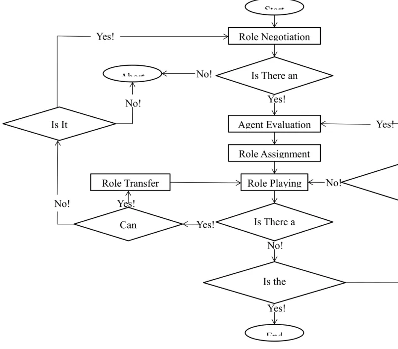
The RBC life cycle consists of three major tasks: role negotiation, role assignment and role execution [40]. Obviously, role assignment is an important aspect of RBC. It greatly affects the efficiency of collaboration and the satisfaction of the members involved in the collaboration. Figure 10 shows the life cycle of RBC.

Figure 10： The life cycle of RBC.

Abort

Role Negotiation

Is There an

Yes!

Agent Evaluation

Role Assignment

Role Playing

Is There a

No!

Is the

Yes!

End

Is

No!

Yes!

Can

No!

Is It

Yes!

Role Transfer

Yes!

No!

Start

No!

(45)

After more than a decade continuous effort, RBC-related research has been developed into a discovery method in the field of collaboration-systems research, including the role transfer problem, the group role assignment problem, and so on.

2.3.2 The Mathematical Formulation of the GRAP

GRAP was first proposed by H. Zhu and R. Alkins in 2009 [76]. It aims at finding the maximum total profit among 𝑛 roles to 𝑚 agents with the agent evaluation result. The unit profit is represented by 𝑃_𝑖,𝑗. Each role can be assigned to more than one agent and one agent can only receive one role.

The mathematical formulation of GRAP is:

{ 𝑚𝑎𝑥 ∑ ∑ 𝑝_𝑖𝑗𝑥𝑖𝑗 𝑛 𝑗=1 𝑚 𝑖=1 (2.3.1) 𝑠. 𝑡. ∑ 𝑥_𝑖𝑗 = 𝐿[𝑗] 𝑛 𝑖=1 𝑗 = 1, … , 𝑛, 𝐿[𝑗] ∈ 𝑁, N is a set of natural numbers; (2.3.2) ∑ 𝑥𝑖𝑗

𝑚

𝑖=1

= 1 𝑗 = 1, … , 𝑛; (2.3.3) 𝑥𝑖𝑗 ∈ {0,1} 𝑖 = 1, … , 𝑚, 𝑗 = 1, … , 𝑛; (2.3.4)

Compared with the mathematical formulation of GAP, the objective function is different which is usually formulated as a maximization problem. The weight 𝑤_𝑖𝑗 becomes uniform for all the agents and 𝑤_𝑖𝑗 = 1. The unit profit 𝑝_𝑖𝑗 is dependent of i and j. The parameter i is allocated to the agent i. The parameter j is allocated to the group role j. The parameters 𝐿[𝑗] (𝑖 = 1, … , 𝑚) represent the minimum numbers of agents required for role j which are integers.

Since GRAP is a well-known hard problem, it needs advanced methodologies, for example information classification, data mining, pattern search and matching [40].

(46)

2.3.3 An Instance of the GRAP

The GRAP has been implemented to a real world problem by Zhu, Zhou and Alkins in 2012 [40]. In a soccer team, there are 20 players (𝑎0~𝑎19) in total. In the field, there are four roles and 11 players for the 1-4-3-3 formation: one goalkeeper (𝑟₀), four backs (𝑟₁), three midfields (𝑟₂), and three forwards (𝑟₃). Figure 11 shows the 20 players and the 4 roles. The coach has to choose 11 players before each game. Players’ performance is evaluated by their modes, emotions, health, fatigue, and past performance.

Figure 11: Soccer team [40]

Assume that the coach has the data shown in Figure 12 to represent the players’ evaluation values for each role (rows represent players, and columns represent roles). By choosing the players, the coach’s goal is to improve the performance of the whole team’s by preparing for role assignment.

(47)

[ 0.65 0.98 0.26 0.33 0.96 0.90 0.59 0.19 0.72 0.61 0.06 0.48 0.19 0.630.43 0.90 0.87 0.35 0.72 0.15 0.06 0.25 0.28 0.01 0.33 0.59 0.75 0.59 0.37 0.670.25 0.45 0.12 0.10 0.84 0.13 0.01 0.510.96 0.63 0.01 0.29 0.07 0.52 0.82 0.120.36 0.95 0.97 0.90 0.14 0.54 0.88 0.540.51 0.26 0.04 0.03 0.44 0.12 0.30 0.91 0.53 0.70 0.48 0.14 0.50 0.06 0.83 0.70 0.16 0.04 0.52 0.96 0.85 0.39 0.76 0.08 0.21 0.85] [ 0 0 0 1 0 0 0 0 0 1 0 0 0 1 0 0 0 0 0 0 0 0 0 0 0 0 0 0 0 0 0 1 0 0 0 0 0 0 0 0 0 0 1 0 0 1 0 0 0 0 0 0 0 0 1 0 0 0 0 1 0 0 0 1 0 0 0 0 0 0 0 1 0 0 0 0 0 0 0 1] (a) (b)

Figure 12: Evaluation values of agents and roles and the assignment matrix [40] The team performance is assumed as a simple sum of the selected players’ performance on their designated roles. The coach has used several strategies to find the exact optimal solution. From 𝑟₀ to 𝑟₃, selecting the best players if they have not been selected. Table 1 shows all the group performances based on several strategies.

Strategy Assignment for {𝒓𝟎}{𝒓𝟏}{𝒓𝟐}{𝒓𝟑} Group

Performance (𝑟0, 𝑟1, 𝑟2, 𝑟3) {12} {0,2,6,15} {9,18,19} {3,11,16} 9.23 (𝑟0, 𝑟1, 𝑟3, 𝑟2) {12} {0,2,6,15} {9,14,18} {3,11,19} 9.30 (𝑟0, 𝑟2, 𝑟1, 𝑟3) {12} {2,6,7,15} {0,9,18} {3,11,19} 9.04 (𝑟0, 𝑟2, 𝑟3, 𝑟1) {12} {2,6,7,15} {0,9,18} {3,11,19} 9.04 (𝑟0, 𝑟3, 𝑟1, 𝑟2) {12} {2,6,7,15} {9,18,19} {0,3,11} 8.98 (𝑟0, 𝑟3, 𝑟2, 𝑟1) {12} {2,6,7,15} {9,18,19} {0,3,11} 8.98 (𝑟1, 𝑟0, 𝑟2, 𝑟3) {18} {0,2,12,15} {9,14,19} {0,3,11} 9.35 (𝑟1, 𝑟0, 𝑟3, 𝑟2) {18} {0,2,12,15} {9,10,14} {3,11,16} 9.41 (𝑟1, 𝑟2, 𝑟0, 𝑟3) {4} {0,2,12,15} {9,18,19} {3,11,16} 9.44 (𝑟1, 𝑟2, 𝑟3, 𝑟0) {4} {0,2,12,15} {9,18,19} {3,11,16} 9.44 (𝑟1, 𝑟3, 𝑟0, 𝑟2) {18} {0,2,12,15} {9,10,14} {3,11,19} 9.41 (𝒓𝟏, 𝒓𝟑, 𝒓𝟐, 𝒓𝟎) {𝟒} {𝟎, 𝟐, 𝟏𝟐, 𝟏𝟓} {𝟗, 𝟏𝟒, 𝟏𝟖} {𝟑, 𝟏𝟏, 𝟏𝟗} 9.51 (𝑟2, 𝑟0, 𝑟1, 𝑟3) {12} {2,6,7,15} {0,9,18} {3,11,19} 9.04 (𝑟2, 𝑟0, 𝑟3, 𝑟1) {12} {2,6,7,15} {0,9,18} {3,11,19} 9.04 (𝑟2, 𝑟1, 𝑟0, 𝑟3) {4} {2,6,12,15} {0,9,18} {3,11,19} 9.25

(48)

(𝑟2, 𝑟1, 𝑟3, 𝑟0) {4} {2,6,12,15} {0,9,18} {3,11,19} 9.25 (𝑟2, 𝑟3, 𝑟0, 𝑟2) {12} {0,9,18} {1,10,14} {3,11,19} 8.79 (𝑟2, 𝑟3, 𝑟2, 𝑟0) {4} {0,9,18} {10,12,14} {3,11,19} 8.98 (𝑟3, 𝑟0, 𝑟1, 𝑟2) {12} {2,6,7,15} {9,18,19} {0,3,11} 8.98 (𝑟3, 𝑟0, 𝑟2, 𝑟1) {12} {2,6,7,15} {9,18,19} {0,3,11} 8.98 (𝑟3, 𝑟1, 𝑟0, 𝑟2) {18} {2,6,12,15} {9,14,19} {0,3,11} 9.10 (𝑟3, 𝑟1, 𝑟2, 𝑟0) {4} {2,6,12,15} {9,18,19} {0,3,11} 9.19 (𝑟3, 𝑟2, 𝑟0, 𝑟1) {4} {2,6,7,15} {9,12,18} {0,3,11} 8.91 (𝑟3, 𝑟2, 𝑟1, 𝑟0) {4} {2,6,7,15} {9,12,18} {0,3,11} 8.91 Table 1:

Comparisons among assignment strategies [40]

By using the enumeration method, the optimal solution is (𝑟₁, 𝑟₃, 𝑟₂, 𝑟₀) as shown in bold row in Table 1. The solution is shown in Figure 12(a) as circles, in Figure 12(b) as a matrix, and in Figure 13 as a graph.

Figure 13: Optimal solution [40]

2.3.4 Concepts

In formalizing GRAPs, 𝑚 expresses the size of the agent, and 𝑛 expresses the size of the role. For example, in the soccer team, m is 20 players, n is four roles as goalkeeper, backs, midfields, and forwards.

Improving group role assignment problem by incremental assignment algorithm

Abstract

Keywords

Acknowledgments

Table of Contents

List of Tables

List of Figures

List of Appendix

Abbreviations

Chapter 1

Assignment Problem

1

1.1

Background

1.2

Perfect Matching

1.3

Bipartite Matching Algorithms

1.3.1

A labeling (dual variables) method to find a maximum matching

1.3.2

Other Algorithms

1.3.3

Applications of the Maximum Matching Algorithm

a

b

c

d

e

f

g

h

a

b

c

d

e

f

g

h

a

b

c

d

e

f

g

h

1.4

Linear Assignment Problem

1.4.1

Linear Sum Assignment Problem

1.4.1.1

Mathematical Model

1.4.1.2

An

𝑂(𝑛

)

implementation of the Hungarian Algorithm

u

v

v

u

u

v

u

v

v

u

u

v

u

v

v

u

u

v

u

v

v