Model predictive torque vectoring control with active trail-braking for electric vehicles

CRANFIELD UNIVERSITY

KONSTANTINOS ZARKADIS

MODEL PREDICTIVE TORQUE VECTORING

CONTROL WITH ACTIVE TRAIL-BRAKING FOR

ELECTRIC VEHICLES

SCHOOL OF AEROSPACE, TRANSPORT AND

MANUFACTURING

Transport Systems

MSc by Research

Academic Year: 2016–2017

Supervisor: Dr E. Velenis and Dr S. Longo

February 2018

CRANFIELD UNIVERSITY

SCHOOL OF AEROSPACE, TRANSPORT AND

MANUFACTURING

Transport Systems

MSc by Research

Academic Year: 2016–2017

KONSTANTINOS ZARKADIS

Model Predictive Torque Vectoring Control with Active

Trail-Braking for Electric Vehicles

Supervisor: Dr E. Velenis and Dr S. Longo

February 2018

This thesis is submitted in partial fulfilment of the

requirements for the degree of MSc by Research.

© Cranfield University 2018. All rights reserved. No part of

this publication may be reproduced without the written

Abstract

In this work we present the development of a torque vectoring controller for electric ve-hicles. The proposed controller distributes drive/brake torque between the four wheels to achieve the desired handling response and, in addition, intervenes in the longitudinal dynamics in cases where the turning radius demand is infeasible at the speed at which the vehicle is traveling. The proposed controller is designed in both the Linear and Nonlin-ear Model Predictive Control framework, which have shown great promise for real time implementation the last decades. Hence, we compare both controllers and observe their ability to behave under critical nonlinearities of the vehicle dynamics in limit handling conditions and constraints from the actuators and tyre-road interaction. We implement the controllers in a realistic, high fidelity simulation environment to demonstrate their performance using CarMaker and Simulink.

Keywords

torque vectoring; MPC; nonlinear predictive control; FEV.

Contents

Abstract v

Table of Contents vii

List of Figures ix

List of Tables xi

List of Abbreviations xiii

Acknowledgements xv

1 Introduction 1

1.1 Motivation . . . 1

1.2 Literature Review . . . 5

1.2.1 Active Chassis Control . . . 6

1.2.2 Electric Motor as Control Actuator . . . 8

1.2.3 Model Predictive Control in Chassis Control . . . 12

1.3 Gap in knowledge . . . 15

1.4 Objectives and Methodology . . . 16

2 Vehicle Modelling 19 2.1 Vehicle Dynamics . . . 19

2.2 Tyre Forces . . . 22

2.3 Powertrain . . . 25

3 Model Predictive Control Fundamentals 29 3.1 Cost Function . . . 32

3.2 State Constraints . . . 33

3.3 Input Constraints . . . 34

4 Linear Torque Vectoring Control Development 37 4.1 Simulation Results . . . 39

4.1.1 Step Steer . . . 39

4.1.1.1 Importance of velocity constraint . . . 39

4.1.1.2 Understeer gradient tuning performance . . . 44

4.1.2 Double Lane Change . . . 44

4.1.2.1 Double Lane Changeµ =0.5 . . . 45

4.1.2.2 Double Lane Changeµ =0.7 . . . 47

4.1.2.3 Double Lane Changeµ =0.9 . . . 50

4.2 Computational Performance . . . 52

4.3 Discussion . . . 54

5 Nonlinear Torque Vectoring Control Development 57 5.1 Nonlinear MPC formulation . . . 57

5.2 Simulation Results . . . 58

5.2.1 Step Steer . . . 58

5.2.2 Double Lane Change . . . 61

5.2.2.1 Double Lane Changeµ =0.5 . . . 61

5.2.2.2 Double Lane Changeµ =0.7 . . . 65

5.2.2.3 Double Lane Changeµ =0.9 . . . 67

5.3 Torque rate expansion . . . 70

5.3.1 Step Steer Results . . . 70

5.3.2 Double Lane Change Results . . . 72

5.4 Computational Performance . . . 78

5.5 Discussion . . . 80

6 Conclusions and Further Research 83 6.1 Concluding Remarks . . . 83

6.2 Future Work . . . 85

List of Figures

1.1 Understeer gradient characteristic . . . 3

1.2 Torque Vectoring technique . . . 5

2.1 Vehicle coordinate system . . . 20

2.2 Four wheel vehicle model. . . 22

2.3 Lateral road coefficient approximation; (a)µmax=0.9, (b)µmax=0.7, (c) µmax =0.5 . . . 26

2.4 Static torque map of YASA-750 motor. [60] . . . 27

3.1 Receding Horizon Control policy. . . 30

3.2 Wheel torque limit calculation block. . . 34

3.3 Torque demand limit calculation block. . . 35

4.1 Velocity, step-steer atT_dmd=1000NmandVin=40k ph. . . 40

4.2 Yaw rate, step-steer atT_dmd=1000NmandVin=40k ph. . . 41

4.3 Position, step-steer atT_dmd=1000NmandVin=40k ph. . . 42

4.4 Wheel torques, step-steer atT_dmd=1000NmandVin=40k ph. . . 43

4.5 Total torque, step-steer atVin=40k phwith a variation ofTdmd. . . 43

4.6 Position responses of different K_und, step-steer at T_dmd =1000Nm and V_in=40k ph. . . 44

4.7 Lateral dynamics CarMaker driver parameters. . . 45

4.8 Yaw rate, double lane change atµ=0.5,Tdmd=700NmandVin=8k ph. 46 4.9 Position, double lane change atµ =0.5,Tdmd =700NmandVin=8k ph. . 46

4.10 Velocity, double lane change atµ =0.5,Tdmd =700NmandVin =8k ph. . 47

4.11 Yaw rate, double lane change at µ=0.7,Tdmd=950NmandVin=8k ph. 48 4.12 Position, double lane change atµ =0.7,Tdmd =950NmandVin=8k ph. . 48

4.13 Velocity, double lane change atµ =0.7 andVin=8k ph. . . 49

4.14 Total torque, double lane change atµ =0.7,Tdmd=950NmandVin=8k ph. 50 4.15 Yaw rate, double lane change at µ=0.9,Tdmd=1150NmandVin=8k ph. 51 4.16 Position, double lane change atµ =0.9,Tdmd =1150NmandVin=8k ph. 51 4.17 Velocity, double lane change atµ =0.9 andVin=8k ph. . . 52

4.18 Total torque, double lane change at µ =0.9, Tdmd =1150Nm andVin = 8k ph. . . 52

4.19 LMPC performance, step-teer atT_dmd =1000NmandV_in =40k ph. . . 53

4.20 LMPC performance, double lane change; top -µ =0.5, Tdmd =700Nm; middle -µ =0.7,T_dmd=950Nm; bottom -µ =0.9,T_dmd=1150Nm. . . 54

5.1 Velocity, step-steer atT_dmd=1200NmandV_in=40k ph. . . 59

5.2 Yaw rate, step-steer atT_dmd=1200NmandVin=40k ph. . . 59

5.3 Position, step-steer atT_dmd=1200NmandV_in=40k ph. . . 60

5.4 Total torque, step-steer atT_dmd=1200NmandV_in=40k ph. . . 60

5.5 Velocity, double lane change at µ=0.5,Tdmd=700NmandVin=8k ph. . 62

5.6 Yaw rate, double lane change atµ =0.5,T_dmd =700NmandVin =8k ph. 62 5.7 Position, double lane change atµ =0.5,Tdmd=700NmandVin=8k ph. . 63

5.8 Total torque, double lane change atµ=0.5,Tdmd=700NmandVin=8k ph. 64 5.9 Velocity, double lane change at µ=0.7,T_dmd=950NmandVin=8k ph. . 65

5.10 Yaw rate, double lane change atµ =0.7,Tdmd =950NmandVin =8k ph. 66 5.11 Position, double lane change atµ =0.7,Tdmd=950NmandVin=8k ph. . 66

5.12 Total torque, double lane change atµ=0.7,T_dmd=950NmandVin=8k ph. 67 5.13 Velocity, double lane change atµ=0.9,Tdmd=1150NmandVin=8k ph. 68 5.14 Yaw rate, double lane change atµ =0.9,Tdmd =1150NmandVin =8k ph. 68 5.15 Position, double lane change atµ =0.9,T_dmd=1150NmandVin=8k ph. 69 5.16 Total torque, double lane change atµ =0.9, Tdmd=1150NmandVin = 8k ph. . . 69

5.17 Velocity, step-steer atT_dmd=1000NmandV_in=40k ph. . . 70

5.18 Yaw rate, step-steer atT_dmd=1000NmandV_in=40k ph. . . 71

5.19 Position, step-steer atT_dmd=1000NmandVin=40k ph. . . 71

5.20 Total torque, step-steer atT_dmd=1000NmandV_in=40k ph. . . 72

5.21 Velocity, double lane change; top - µ =0.5, Tdmd =700Nm; middle -µ=0.7,Tdmd=950Nm; bottom -µ=0.9,Tdmd=1150Nm. . . 73

5.22 Yaw rate, double lane change; top - µ =0.5, T_dmd =700Nm; middle -µ=0.7,Tdmd=950Nm; bottom -µ=0.9,Tdmd=1150Nm. . . 75

5.23 Position, double lane change; top - µ =0.5, Tdmd =700Nm; middle -µ=0.7,T_dmd=950Nm; bottom -µ=0.9,T_dmd=1150Nm. . . 76

5.24 Total torque, double lane change; top -µ =0.5,Tdmd=700Nm; middle -µ=0.7,Tdmd=950Nm; bottom -µ=0.9,Tdmd=1150Nm. . . 77

5.25 NMPC performance, step-steer atT_dmd=1000NmandV_in =40k ph; Left images - torque rates NMPC; Right images - wheel torques NMPC. . . . 78

5.26 NMPC performance, double lane change; top -µ =0.5,Tdmd=700Nm; middle -µ =0.7,T_dmd=950Nm; bottom -µ =0.9,T_dmd=1150Nm. . . 79

5.27 NMPC dT performance, double lane change; top -µ=0.5,Tdmd=700Nm; middle -µ =0.7,Tdmd=950Nm; bottom -µ =0.9,Tdmd=1150Nm. . . 80

List of Tables

2.1 Vehicle properties. . . 22 3.1 Motor specs in simulation. [1] . . . 36

List of Abbreviations

4WS Four Wheel Steering ABS Anti-lock Braking System AFS Active Front Steering

ATTS Active Torque Transfer System AWD All-Wheel Drive

AYC Active Yaw Control CC Cruise Control CM Centre of Mass DoF Degrees of Freedom DYC Direct Yaw Control EM Electric Motor EoM Equations of Motion

ESP Electronic Stability Program EV Electric Vehicle

FWD Front-Wheel Drive HEV Hybrid Electric Vehicle ICE Internal Combustion Engine LTV Linear Time Varying

LQG Linear Quadratic Gaussian xiii

LQR Linear Quadratic Regulation MF Magic Formula

MPC Model Predictive Control

NMPC Nonlinear Model Predictive Control PDIP Primal-Dual Interior Point

PID Proportional Integral Derivative QP Quadratic Program

RHC Receding Horizon Control RWD Rear-Wheel Drive

SATM School of Aerospace, Transport and Manufacturing SH-AWD Super Handling All-Wheel Drive

SMC Sliding Mode Control SUV Sport Utility Vehicle TCS Traction Control System UKF Unscented Kalman Filter

Acknowledgements

I would first like to thank my supervisors Drs. Efstathios Velenis and Stefano Longo for introducing me into the vehicle dynamics and MPC world respectively as well as for all the guidance through this research work. I would also like to thank Drs. Siampis, Sofian who were always by my side supporting my research with their valuable knowledge and experience.

Finally, I express my thanks to my family and my girlfriend ”K” for supporting and encouraging me through the process of my research and writing this thesis. This accom-plishment would not have been possible without them.

A special gratitude to the Autolads. Thank you all.

Chapter 1

Introduction

1.1

Motivation

Chassis control systems have been in the centre of research many decades, controlling the longitudinal, lateral and vertical motion of the vehicle in order to improve handling and acceleration\braking behavior [21]. This subject area growing fast nowadays due to the increased safety concerns rising from the increasing number of automobiles on the road in combination with higher performance. Additionally, the rapid development in the microprocessor computing field is offering faster and cheaper platform solutions for chassis control deployment.

In 1978, the introduction of the Anti-lock Braking System (ABS) was one major breakthrough and now is a standard basic feature of every vehicle. A few years later another chassis control system was introduced, the Traction Control System (TCS),

panding the ABS by including slip control during acceleration [34]. Later on, more con-trol systems came to light such as Four Wheel Steering (4WS), active suspension and braking systems like Electronic Stability Program (ESP) [58].

Losing control of a car in a corner is dangerous. Ideally, a car should be able to ne-gotiate the corner under control with neither excessive oversteer or understeer. However, taking a corner too fast, performing an emergency maneuver, bad weather, defective road surfaces or poor maintenance of the car may result in a loss of grip leading to a loss of control. Systems that control the lateral dynamics, in such scenarios, mainly focus on improving the steerability of the vehicle and preventing the driver from losing control in limit handling conditions. On the other hand, longitudinal vehicle control is commonly regulated under the command of the driver with systems such as Cruise Control (CC) in which, recently, safety functions for vehicle speed regulation have been integrated, to keep a safe distance from the front vehicle. However, it is recognised that active con-trol of longitudinal dynamics can improve the vehicle’s stability in terminal understeer situations.

Understeer, oversteer and neutral steer are terms used to describe the vehicle’s re-sponse to steering inputs. Due to the complexity in the relation between the steering angle on the wheels and the response of the vehicle, the concept of the understeer gradientK_und

has been introduced. Assuming a single-track model under steady state cornering with all tyres at their linear region operation, the understeer gradient gives an indication of the natural behavior of the vehicle under a constant steering input from [49]

δ = L

R+Kunday, (1.1)

whereδ is the front wheels’ steering angle,Lis the vehicle’s wheelbase,Ris the vehicle’s

path radius anda_y=Vx2

1.1. MOTIVATION 3 The three cases are:

• K_und =0, neutralsteer, no need to vary the steering angle ,

• K_und>0, understeer, the steering angle has to be increased according to the second term of (1.1) in order to keep a constant radius path, with a characteristic speed

V_char being the speed at which the steering angle is double the Ackerman angle

δacker= L_R [23] as shown in Fig1.1

• K_und<0, oversteer, the steering angle has to be decreased while the speed increases until the vehicle reaches the critical velocityV_crit and the steering angle is zero

δ Vx VcharVcrit neutralsteer oversteer understeer L R 2_RL

Figure 1.1: Understeer gradient characteristic

Despite the fact that the understeer gradient can quantify the natural tendency of the ve-hicle to follow a path radius or not, it is important to note that the veve-hicle’s behavior can change while cornering due to the its drivetrain topology and use of acc\brake pedal. This derives from the longitudinal and lateral tyre force coupling effect in which the lateral tyre force reduces when the longitudinal tyre force increases.

Understeer usually occurs when the front wheels reach the tyre’s cornering stiffness limit and lose grip earlier than the back wheels, resulting in the car continuing straight

instead of turning. Most Front Wheel Drive (FWD) cars tend to understeer when acceler-ating out of a bend, mostly because the front tyres do the job of acceleration-deceleration and steering. Approaching a corner faster than what the tyres can support, causes the front tyres to struggle to keep the car in line, and try to steer the car in a direction you’re pointing it to.

Oversteer is the opposite of the understeer where the rear tyres lose grip while the front wheels remain bellow the limit of adhesion. Rear Wheel Drive (RWD) cars, on the other hand are less prone to understeer, because the front wheels do the steering and the rear ones the driving. Accelerating hard out of a bend in a RWD car could cause it to oversteer due to the rear wheels running out of grip from the power being delivered and the turning of the car.

Therefore, returning to the limit handling scenarios, terminal understeer refers to a vehicle in which the front tyres potential lateral force is at a maximum due to excessive vehicle speed while cornering. In [68] the importance of a velocity regulation is men-tioned as a performance requirement for the development of ESP system by Bosch.

Electric Vehicles (EV) have gained a lot of popularity the last years not only for their important role as environmentally friendly transportation but also for their increased per-formance in traction and stability systems. Having the ability of different propulsion system configurations, such as independent motors for each wheel, electric vehicles allow us to implement more efficient safety algorithms [7, 64].

One of the most trending algorithms is Torque Vectoring (TV) which controls the wheel torque distribution respecting as closely as possible the drivers steering wheel and throttle/brake commands to improve the passengers safety. To be more precise, TV sys-tems aim at controlling the lateral dynamics of the vehicle by tracking the yaw rate and occasionally the side slip angle reference signals while at the same time following closely the torque demand input given by the driver using the pedals. As shown in Fig.1.2 the

1.2. LITERATURE REVIEW 5 vehicle consists of four independent electric motors, each one driving a wheel. Since the driver’s intention is to turn left, as shown from the yaw momentM_z, the torque vectoring control algorithm sets the appropriate torque values on each wheel. Therefore the wheel torques on the outer side of the turning vehicle are positive and on the inner side are nega-tive. Torque Vectoring is used in sublimit cases to deliver customisable handling behavior and can act as stability control as the tyres reach their adhesion limit.

Figure 1.2: Torque Vectoring technique

1.2

Literature Review

The literature of the most important vehicle chassis control solutions in both the automo-tive industry and academia, is being split into lateral and longitudinal dynamics control systems.

1.2.1

Active Chassis Control

In AVEC ’92 a number of papers were presented for the first time refering on the use of left-right tyre force distribution to control the vehicle’s lateral dynamics [21]. One of the studies which made a debut was theβ-method emphasising the role of side-slip

an-gle under acceleration\braking while cornering [59]. The results not only showed that yaw moment gain decreases while sideslip angles increase thus influencing the vehicle’s maneuverability, but also that the yaw moment ”shifting” to high values can change a vehicle’s behavior from neutralsteer to understeer during acceleration and the opposite during deceleration. A final note in [59] indicates that yaw moment gain under steady-state cornering can be expressed as a function of both longitudinal and lateral acceleration and through the use of a hypothetical external yaw moment the influence of that accelera-tion and deceleraaccelera-tion can be eliminated. This method is called Direct Yaw Control (DYC) and was applied on an All Wheel Drive (AWD) vehicle where the external yaw moment was expressed as a distribution of the traction and braking forces on the rear wheels, while keeping the front-rear distribution constant. The results showed the effectiveness of the method and popularised the brake stability systems by the late 90s.

The most popular types of DYC application so far are [43]:

• lateral braking control, which uses independent braking between the left and right side of the vehicle to generate a yaw moment

• torque distribution control, which splits the engine’s torque between left and right wheels resulting in a driving torque difference between them hence a yaw moment generation

• torque vectoring control, which transfers torque from left side wheels to right side ones or vice versa, in order to create a braking torque on one wheel while at the

1.2. LITERATURE REVIEW 7 same time transferring an equal amount of driving torque to the other side wheel.

Using braking to control the lateral dynamics of the vehicle, hence ”lateral” brak-ing control, is effective across a wide range of vehicle operatbrak-ing conditions, makbrak-ing it widely used in limit handling scenarios where stability is more important than comfort, but creates a negative feeling on the driver due to the deceleration of the vehicle [43]. The most successful system under this category is Bosch’s ESP [40] with other car man-ufacturers following their example such as Ford [67] and BMW [38]. Other studies that include lateral dynamics braking control are [6], where aH_∞controller uses Active Front Steering (AFS) and and differential braking to achieve the yaw rate and sideslip angle targets, [66], which uses a Sliding Mode Control (SMC) strategy for yaw rate and sideslip control while taking into account variations in the longitudinal dynamics, and [31] which uses throttle control and differential braking to manipulate the slipping condition of the rear tyres according to a yaw rate target on a RWD vehicle.

The last two DYC techniques mentioned above, quickly gained popularity against the lateral braking control due to their less intrusive character in sub-limit conditions. Systems with lateral torque distribution are mainly active differentials that regulate the direction of torque to the left and right wheels under both limit and sub-limit conditions but their main disadvantage is that they cannot generate a corrective yaw moment when the engine torque in not large enough, for example when the vehicle is decelerating [43], or when the engine torque is zero [53]. The most successful example is the Active Torque Transfer System (ATTS) from Honda [57] which shows improved stability and handling during a combination of steering and acceleration\deceleration inputs. In the case of torque vectoring control, the torque transmitted between the wheels does not conflict with the driver’s acceleration and braking commands although it can have a negative effect on the vehicle’s steering wheel action when it’s applied on the front axle. The most

popu-lar example is the Active Yaw Control (AYC) system from Mitsubishi and its successor the Super AYC [74]. They use a mechanism which transfers and controls the rear wheel torques under different driving conditions, limiting the vehicle’s yaw moment and en-hance its cornering performance. AYC can also act like a limited slip differential by containing rear wheel slip to improve traction.

Torque distribution, nowadays, has also found its way into the AWD vehicles. In [46, 47], Piyabongkarn showed that front-rear torque distribution can change the under-steer characteristiccs of the vehicle, although it is not as effective as left-right distribu-tion. A representative example is a series of papers from Ricardo developing a centre differential for a Sports Utility Vehicle (SUV), where experiments in a BMW X5 showed mixed results [72] and led to a left-right differential change instead in [71]. Distribution of the torque to all four wheels gives better traction compared to a FWD\RWD solu-tion and the cornering performance can be improved without interfering with the driver’s throttle\brake inputs [55]. The most characteristic example is the Super Handling AWD (SH-AWD) system implemented by Honda which combines a set of electromagnetic clut-shes to vary the front-rear distribution and an improved variant of the ATTS to vary the left-right distribution in a single unit at the rear axle. Experimental results showed less understeering behavior when the SH-AWD system was used but when the vehicle was off-throttle it was not possible to transfer torque between wheels [36].

1.2.2

Electric Motor as Control Actuator

The rapid development of both Electric Vehicles (EV) and Hybrid Electric Vehicles (HEV) has already presented exciting new possibilities on the vehicle dynamics area. Both EVs and HEVs have attracted attention not only as response to the increasing fuel prices and the growing environmental concerns but also because EMs deliver both tractive and

brak-1.2. LITERATURE REVIEW 9 ing torque. Depending on vehicle topology we can distribute torque between front/rear axles, left/right wheels of one axle, or all 4 wheels therefore eliminating the distinction between the different control strategies documented above (braking, torque distribution and torque vectoring) thanks to the use of the electric motor.

Most of the research has been focused on the energy management and powertrain technology challenges [11]. However, the electirc motor has some distinct advantages over the conventional drivelines [26, 28, 52]:

• extremely quick and accurate response and can be controlled according to speed or torque demand

• dual operation, can be used as a motor or a generator with almost equal efficiency

• high energy efficiency up to 90%

• in the case of in-wheel motors the powertrain architecture is simplified with less mechanical parts giving also way to new passenger cell designs

Despite the advantages mentioned above, there are a few risky questions left. While the fundamentals of vehicle dynamics do not need to be redefined, certain challenges come to light when the powertrain is changed from a conventional Internal Combastion Engine (ICE) to an electric one. The most important ones are the increased sprung mass and packaging constraints related to the necessary inclusion of the battery and the in-creased unsprung mass and suspension packaging in the case of in-wheel motors, both investigated from Crolla and Cao [12]. Extra load from the battery can impact roll sta-bility, ride vibration and comfort while the increase of unsprung mass makes the vertical wheel motion more challenging. It is obvious that there are clear advantages and disad-vantages using an electric motor as the main actuator and both academia and automotive

industry are actively looking at appropriate solutions along with the increased government interest over the years.

A meaningful amount of torque vectoring examples on EVs can be found in literature. In [51] a SMC strategy is used with the driver steering input modeled as a disturbance, and in [75] a Linear Quadratic Gaussian (LQG) controller, used to enhance steerability within a given yaw and sideslip control region or maneuverability outside it. In the case of AWD EVs one of the earliest examples is presented from Hori Laboratory in Tokyo University [26] where they implemented ABS and TCS on an EV and later extended to yaw rate tracking [22, 44]. Other drivetrain topologies and control methodologies found in literature include an integrated torque control of a rear electric motor and the electro-hydraulic brake system using a fuzzy logic controller in [33], an adaptive controller on a system with independent rear in-wheel motors and AFS [8] and a rather unique EV concept developed by the Technical University of Munich called MUTE, where apart from the main electric motor there is also a second one superimposed in the rear differential to obtain torque vectoring capabilities [25]. Another study controlling the lateral vehicle dynamics can be found in [45] where they use a Proportional-Integrated-Derivative (PID) controller to calculate the requests on the two rear axle electric motors for yaw rate and sideslip angle error minimisation from target values set by a bicycle model.

A characteristic example of torque vectoring control can be found from the 7FP EU project E-VECTOORC [3] where they employed a control allocation scheme for torque vectoring of a four electric motors pure EV. The main aim of the project was to create a fun-to-drive vehicle while at the same time improving energy efficiency using torque modulation for brake energy recuperation, ABS and TCS functionality. In [27] an ap-propriate cost function is presented for the control of the vehicle dynamics while in [13] Novellis et al. focus on the control allocation problem using an offline optimisation al-gorithm using a range of different cost functions based on performance and power usage

1.2. LITERATURE REVIEW 11 criteria. The authors conclude that slip-based cost functions are highly recommended for control allocation of the wheel torques in EV applications. Finally they extended their pre-vious work adding a sideslip angle control strategy which activates a sideslip-based yaw moment contribution when the sideslip angle value exceeds a pre-defined threshold [14].

Until now, the longitudinal dynamics control of the vehicle has largely remained un-der the full authority of the driver being restricted in systems such as the CC for comfort reasons and in autonomous vehicle control applications. In addition, braking systems for DYC that decelerate the vehicle are mostly viewed as depreciating on the driving expe-rience [46, 54]. Although it is well known that the driver should remain at the centre of the longitudinal dynamics control, later research has proven that active control can im-prove the stability in limit handling situations [24, 39]. Terminal understeer arises when an overspeeding vehicle enters a turn and its turning radius cannot be decreased to match the minimum turn-radius given by its velocity and understeer gradient. One of the earliest studies which explored this idea is [35] where they noted that stability and path tracking is improved with the combination of a corrective yaw moment and braking through appro-priate brake control of the four wheels. More recently, Rajamani and Piyabongkarn [50] concluded that a reduction of lateral acceleration by decreasing the velocity of the ve-hicle before entering a sharp turn provides a better cornering performance and rollover mitigation than a typical yaw rate controller. Reduction of lateral acceleration results in reduction of slip angle at the tyres and lower chances of exceeding the limit of adhesion.

A more interesting EV implementation of active longitudinal dynamics control can be found in [61]. Here, a combined solution of yaw stabilisation and velocity regulation for terminal understeer mitigation is presented. The controller is an extension of a previous work [69] which consisted of a Linear Quadratic Regulator (LQR) with the steering angle and the angular rate of the rear wheels as inputs. In addition, they extended the control ar-chitecture to contain a rear axle torque vectoring configuration, considering independently

driven rear wheels and taking into account the requested turning radius in agreement with the velocity of the vehicle.

1.2.3

Model Predictive Control in Chassis Control

Model Predictive Control (MPC) models are mainly solving complex dynamical systems. This complexity occurs due to large time delays and high-order dynamics where PID con-trollers have a difficulty solving. Recently, the emergence of MPC and efficient numerical algorithms, has made it possible for such techniques to be used in vehicle chassis control applications, delivering optimal solutions and incorporation of critical constraints in the calculation of the control action.

In the automotive research and development sector, a variety of MPC solutions can be found in the literature, ranging from steering control [18] to semi-active suspension con-trol [10], longitudinal following concon-trol of autonomous vehicles to achieve vehicle pla-toons [48] and emission regulation [56]. Looking closer in our area of interest, the area of vehicle dynamics control, we distinguish two major MPC application areas, autonomous\ semi-autonomous vehicle control and active safety control systems. However, due to the rapid improvement of sensor technologies and sensor fusion algorithms, the distinction between those two application fields is becoming ambiguous nowadays.

From the autonomous vehicle applications perspective, a series of papers have been presented from Borrelli and Falcone [9, 17–20] and Keviczky [32], exploring the applica-tion of MPC for trajectory tracking in an autonomous vehicle applicaapplica-tion using the AFS system with/without differential braking and traction control. In [9, 32] both authors im-plemented a nonlinear MPC (NMPC) strategy for tracking a determined trajectory using the AFS of an autonomous vehicle which, according to the authors, sets the benchmark for future sub-optimal strategies. Since the problem with the NMPC strategy was that it

1.2. LITERATURE REVIEW 13 could not be implemented in real-time, in [18], Falcone et al. presented a Linear Time Varying (LTV) MPC linearising the NMPC problem from [9, 32] about the operating point. Simulation and experimental results show no infeasibility issues in high veloci-ties but are suffering in tracking performance compared to the NMPC formulation. In the next two papers [17,19] they integrated more functions in the MPC including independent wheel braking and active front and rear differentials. Another distinction from the previ-ous work is the replacement of the bicycle model by a four-wheel vehicle model in [19], although the effect of load transfer is still not taken into account. The goal of the MPC is to follow a predefined trajectory as before but also follow a given velocity reference. The double lane change simulations on a low-µ road surface show a comparison of

dif-ferent drivetrain topologies, one which includes AFS with braking and traction control, another which neglects traction control and finally one including AFS only. As for the test results, it is interesting to note that the reference velocity used is set equal to the initial velocity of the vehicle, thus a speed decrease is observed due to the vehicle reaching a terminal understeer condition. From the above results, the authors concluded the solution that combines AFS with braking and traction control has the best overall performance but the best lateral position tracking is achieved by the solution that uses AFS with braking control only.

In the final work of the series [20] the authors constructed two NMPC strategies, one employing a four-wheel vehicle model with wheel dynamics and control inputs the front steering and individual wheel brake torques and another one that uses a bicycle model instead, with a direct yaw moment along with AFS as control inputs. Although simulation tests on a double-lane change show promising results, once again the main problem for both controllers remains to be the high computational cost, making them impossible for real-time implementation. For that reason, a third controller is developed which uses a linearisation of the first, more complex, controller about the operating point and tested on

a vehicle with rather good path tracking results. All three controllers showed some trade-offs exhibiting certain advantages and disadvantages, although a recurring topic seems to be the importance of good tuning.

In the field of active safety control systems there is plenty of literature too, varying from yaw stability controllers using independent braking of the four wheels based on a LTV-MPC strategy [5] and hybrid MPC [15], to slip controller using torque blending of both electric and hydraulic brake torque [7] and torque vectoring algorithm to achieve minimum time performance maneuvering [64]. Having a closer look at Basrah et al. [7], they employed both linear and nonlinear MPC strategies integrating a slip controller and torque blending between both electric and hydraulic braking actuators. The internal model used in the MPC algorithm is a single-wheel model consisted of longitudinal acceleration, angular wheel rate and the total amount of wheel torque equal to the summation of electric and hydraulic torque. For the calculation of the tyre force they use a simplified version of Pacejka’s Magic Formula (MF) which contains the controlled longitudinal slip to compute the longitudinal force, and neglect the lateral movement of the vehicle. Simulation results show that the linear MPC suffers from poor performance at low speeds compared to the nonlinear one, but both controllers track the slip reference target in a similar way for most of the braking maneuver. A solution to that poor performance is proposed by reducing the sampling time of the linear MPC, however the computational performance is worsened making the controller not implementable in real-time. One interesting observation was made under the split µ simulation maneuver where the vehicle maintains stability and

steerability throughout the braking with sufficient countersteering by the CarMaker driver model.

1.3. GAP IN KNOWLEDGE 15

1.3

Gap in knowledge

A series of torque allocation techniques including predictive control have been done by Khajepour et al. from the University of Waterloo in collaboration with General Motors (GM). In [30] they deployed a linear MPC technique using recursive linearisation of the vehicle dynamics, to achieve the desired handling response (yaw rate) by distributing the torque demand in the four wheels of an electric vehicle. Later, in [29] they expanded their work by adding a velocity estimation method which treats acceleration measurement noises and road conditions as uncertainties, implementing an Unscented Kalman Filter (UKF). Longitudinal and lateral tyre forces are assumed to be known from the Kalman Filter estimation without requiring the road friction coefficient. The MPC calculates the appropriate wheel torque according to the yaw rate, the yaw moment of the lateral tyre forces and the wheel speed tracking errors. Then they feed the torque change for each wheel from the current driver’s torque demand, based on the accelerator pedal position, to the vehicle. The real-time results in both [29] and [30] show effective handling and stability performances tested on a four electric motor wheel vehicle under several driving scenarios.

In [63] a combined yaw stabilization and velocity regulation is presented to mitigate terminal under-steer using rear axle electric torque vectoring. The vehicle model incorpo-rates nonlinear tyre characteristics and coupling of the longitudinal and lateral tyre forces and linear MPC designs are presented using recursive linearisation of the vehicle dynam-ics. Recently, the control design from [63] has been extended to nonlinear MPC in [62] and compared with previous linear approaches, both in terms of control objective achieve-ment and demanded computational resource. It is worth noting that the control scheme of both [63] and [62] does not take into consideration any torque demand by the driver. The controller aims at stabilizing the lateral dynamics of the vehicle and tracking a speed

ref-erence determined from the steering input of the driver in order for the requested turning radius to be feasible. In addition, this approach does not consider the modification of the handling behavior of the vehicle, as for instance in [14] where the understeer gradient of the controlled vehicle is actively modified by the torque vectoring system.

In this research study we present the development of a torque vectoring controller to distribute the requested drive/brake torque to the four wheels of an electric vehicle to control the longitudinal and lateral dynamics. In addition to the approaches of [30] and [14], which are close to the classic torque vectoring, the controller is designed to intervene to the longitudinal dynamics of the vehicle in cases of overspeeding in a cor-nering maneuver, thus having a protection on terminal understeer. The controller delivers an on-demand modified lateral dynamics response and aims to deliver the torque demand set by the driver in addition to the approach of [63] and [62]. We employ a NMPC design which accounts for vehicle dynamics nonlinearities and actuator limitations. In addition, the longitudinal intervention is integrated into the control design by introducing a feasible velocity constraint, rather than tracking a velocity reference as in [63] and [62]. The con-troller is implemented in a high fidelity simulation environment, IPG Carmaker [2], where its performance is demonstrated and the real time implementation capability is discussed.

1.4

Objectives and Methodology

The aim of this research is to develop a real-time implementable torque vectoring control algorithm for electric vehicles with a limit case scenario expansion for limit handling con-ditions. The attention is focused on a specific vehicle, the Delta Motorsport E-4 Coupe which is a AWD electric vehicle with four electric motors each commanding one wheel. The final solution will be able to stabilise the vehicle under any sub\limit handling con-dition including oversteer cases.

1.4. OBJECTIVES AND METHODOLOGY 17 In order to meet this objective, some contributions must be achieved first:

• develop a computationally simple yet accurate vehicle model to produce the refer-ence signals needed for the controller to follow

• develop an unconstrained linear optimal control to observe the torque vectoring behavior

• develop a constrained version of the previous controller showing the importance of the velocity regulation under limit case scenarios

• expand the constrained controller to nonlinear and analyse both advantages and disadvantages

• compare both linear and nonlinear optimal controllers’ computational computer real time performance

It is important to note at this point that all the developed strategies will be systemat-ically assessed in terms of real-time feasibility, since in the context of vehicle dynamics control strategies like the ones presented here it is important to make sure that all solu-tions are real-time implementable. The simulation studies are made on a laptop computer (i7-4710HQ at 2.50 GHz with 16 GB of RAM memory).

Chapter 2

Vehicle Modelling

2.1

Vehicle Dynamics

In this section we provide the vehicle dynamics model which is used to calculate the opti-mal control inputs by the Model Predictive Controller presented in the following section. As mentioned in the introduction, the controller is aimed to intervene in both longitudinal and lateral dynamics and hence longitudinal, lateral speed and yaw rate are the selected state variables of the model.

A three Degrees of Freedom vehicle model is used in this study where its Equations of Motion (EoM) are expressed in a coordinated frame attached to the center of mass as shown in Fig. 2.1. Similar to common practice [60, 70], in order to reduce the complexity of the model certain assumptions are made, neglecting:

• the Ackerman Principle, therefore both front wheels steer with the same angle • the rolling resistance

• the suspension dynamics • pitch and roll motion of vehicle

• the transmission and brake system characteristics • the aerodynamic forces

z

x y

Figure 2.1: Vehicle coordinate system

Using Newton’s 2nd Law in the longitudinal and lateral direction we derive the Equa-tions of Motion:

ma_x=

∑

may=

∑

2.1. VEHICLE DYNAMICS 21 where a_x,a_y are the longitudianl and lateral accelerations respectively and can be ex-pressed in terms of the corresponding velocitiesV_xandV_y and the yaw rateras follows:

ax=V˙x−rVy,

a_y=V˙_y+rV_x

(2.2)

Additionally, including the rotational part of the Neuton-Euler equations and the an-gular rate dynamics of the four wheels, the EoM for the four wheel vehicle model are:

mV˙_x= (f_FLx+f_FRx)cosδ−(fFLy+fFRy)sinδ+fRLx+fRRx+mrVy, (2.3a)

mV˙y= (fFLx+fFRx)sinδ+ (fFLy+fFRy)cosδ+fRLy+ fRRy−mrVx, (2.3b)

I_zr˙=l_F[(f_FLx+f_FRx)sinδ+ (fFLy+fFRy)cosδ]−lR(fRLy+ fRRy)

+w_L(−f_FLxcosδ+ fFLysinδ−fRLx) +wR(fFRxcosδ−fFRysinδ+fRRx), (2.3c)

wheremis the mass of the vehicle, δ is the steering angle on both the front wheels,

I_z is the vehicle’s moment of inertia about the vertical axis and ˙r is the vehicle’s yaw moment. The longitudinal and lateral tyre forces are denoted by f_{i jk}wherei=F,R(Front, Rear), j=L,R(Left, Right) and k=x,y. Finally, the distances l_F,l_R,w_L,w_R determine the location of the center of each wheel with respect to the CoM as shown in Fig.2.2.

In the EoM above we consider the steering angle as a parameter provided by the driver. The longitudinal tyre forces are calculated from wheel torque rate control inputs and vertical wheel loads whereas the lateral tyre forces are provided as functions of the corresponding tyre slip angle as described in the following section. All the parameters used for the vehicle and tyre model can be seen in Table 2.1.

Figure 2.2: Four wheel vehicle model.

Table 2.1: Vehicle properties.

Parameter (Unit) Description Value

m(kg) mass 1137

L(m) wheelbase 2.5

R_w (m) wheel radius 0.298

h(m) height of C.M. 0.317

I_z (kg·m2) yaw inertia of vehicle 1174

l_F (m) front axle to C.M. distance 1.187

l_R(m) rear axle to C.M. distance 1.313

w_L(m) left wheels to C.M. distance 0.687

w_R (m) right wheels to C.M. distance 0.687

2.2

Tyre Forces

By neglecting the pitch and roll rotation along with the vertical motion of the sprung mass of the vehicle, the vertical force f_{i jz} on each wheel is calculated using the static load

2.2. TYRE FORCES 23 distribution and longitudinal and lateral weight transfers [69]:

fFLz= fFLz0 −∆fLx−∆f y F, f_FRz= f_FRz0 −∆f_Rx+∆f_Fy, f_RLz= f_RLz0 +∆f_Lx−∆f_Ry, fRRz= fRRz0 +∆fRx+∆f y R, (2.4) ∆f_Fy = mhlR (l_F+l_R)(w_L+w_R)ay, ∆f_Ry= mhlF (l_F+l_R)(w_L+w_R)ay, ∆f_Lx= mhwR (l_F+l_R)(w_L+w_R)ax, ∆f_Rx= mhwL (l_F+l_R)(w_L+w_R)ax, (2.5)

where f_{i jz}0 is the static vertical force distribution,∆f_Fy and∆f_Ry the weight transfer along

the lateral body axis resulting from lateral acceleration a_y and ∆f_Lx and ∆f_Rx the weight

transfer along the longitudinal body axis resulting from longitudinal accelerationax.

As mentioned before the longitudinal forces in EoM (2.3a) - (2.3c) are considered as the control inputs of the vehicle dynamics. In the literature TV controllers deliver wheel force (or torque) commands. A low level controller then is applied to provide the commanded wheel forces, controlling the wheel dynamics. In the proposed method we assume knowledge of the friction coefficient between the tyre and road (µ) and use this

as a constraint on the individual wheel force command. Hence the demanded force is always feasible, although there will be a delay between applied torque and wheel force associated with the wheel inertia. For simplicity and computational efficiency we do not implement a low level controller for wheel dynamics, however the controller is validated

in the following using a rich vehicle model including wheel dynamics as well as the elec-tric motor’s dynamics. Assume we can control longitudinal forces of the tyre directly we can associate the normalised longitudinal tyre forces µi jx with the applied wheel torques

as follows [30]:

µi jx=

Ti j

fi jzRw

, (2.6)

whereTi j is the torque of each wheel andRwthe wheel’s radius.

Next we introduce a model for the calculation of the lateral tyre forces, which includes the dependence on tyre slip angle (cornering stiffness), a linear dependency on the normal force and the coupling with the longitudinal tyre forces.

Using the friction circle concept, the maximum lateral tyre force coefficient µ_{i jy}max is

given by the tyre-road friction coefficient mu and the controlled longitudinal tyre force coefficientµi jx:

µ_{i jy}max= q

µ2−µ_{i jx}2 . (2.7)

Neglecting wheel dynamics and tyre force dependency on slip, we assume direct con-trol of longitudinal forces. We are still able to incorporate the friction circle constraint. The lateral force coefficient is then calculated as a linear function of the tyre slip angle, saturated by the aboveµ_{i jy}maxlimit.

µi jy=sign(αi j)·min(µi jymax,ni j|αi j|), (2.8)

where αi j is the slip angle at each of the four tyres, and ni j is the cornering stiffness

coefficient of each tyre defined as the ratio of tyre cornering stiffness divided by the normal force at each tyre.

2.3. POWERTRAIN 25 In order to avoid the non-smoothness at the point of saturation in equation (2.8), we propose to use an approximation of this expression using the Logistic function [37] as follows: µi jy= 2µ_{i jy}max 1+e−kniαi j −µ max i jy . (2.9)

In the above equation k is the steepness of the curve and is tuned according to the cornering stiffness coefficient of the tyre. To be more precise, we simulated the tyre model under the same road friction coefficient but different understeer gradients, found the best match for the variablek in each case and then calculated a curve that fits those points using MATLAB’s ”fit” command. Thekas a function ofµ_{i j}maxis:

k(µ_{i j}max) = (p1·(µ_{i j}max)2+p2·µ_{i j}max+p3) (2.10)

wherep₁=5.179, p₂=−12.37 and p₃=9.429.

As we can see in Fig.2.3 the saturating equation (2.9) not only follows the boundaries but is smoother than the one corresponding to (2.8). Finally, the longitudinal and lateral tyre forces are calculated using the normal force at each tyre as follows:

f_{i jx}= f_{i jz}µi jx and fi jy= fi jzµi jy (2.11)

2.3

Powertrain

In a vehicle, the powertrain portrays the fundamental components that generate power and drive it to the road surface. This incorporates the motor, transmission, drive shafts,

−1 −0.5 0 0.5 1 −1 −0.5 0 0.5 1 α (rad) µ y

piece-wise linear model smooth approximation (a)

(b) (c)

Figure 2.3: Lateral road coefficient approximation; (a) µmax =0.9, (b) µmax =0.7, (c) µmax=0.5

differentials, and the final drive. In the last decade more elements have been added to the powertrain group due to the emergence of electric and hybrid vehicles, such as the battery, the electric motor and the control algorithm.

The powertrain used in this study is based on an electric vehicle with four individual electric motors (EM). Each EM delivers torque to one wheel limited by the producer’s specs. In our case the electric vehicle used for the simulations is based on the Delta E4-coupe, a prototype vehicle manufactured by Delta Motorsport [1], a company based in Silverstone circuit. Their vehicle has four individual YASA electric motors with maxi-mum and minimaxi-mum torquesTmax=750NmandTmin=−500Nmrespectively. The vehicle

is also equipped with every necessary measurement sensors all road vehicles include. The torque vectoring control algorithm we employ is deeply focused on pure electric vehicle control, however the vehicle features hydraulic brakes on each wheel for safety reasons. As shown in Fig.2.4 the static torque of the YASA-750 electric motor is not con-stant but changes according to its rotational speed, making it important to include torque

2.3. POWERTRAIN 27 constraints in the controller. The control scheme we are implementing is respecting the EM torque limits and can be easily reconfigured to work with different brand manufac-turers without losing its robustness.

Chapter 3

Model Predictive Control Fundamentals

Model Predictive Control is an optimisation based control law which utilises an interior model of the procedure, a measured history of the past control inputs and an optimisation cost functionJover a receding prediction horizon. MPC, is also called Receding Horizon Control (RHC). This control algorithm computes the necessary control inputs for the plant every time step. To be more precise, it solves an omptimisation problem for the current prediction horizon, then applies the first value of the computed control sequence to the plant and finally gets the system state and recomputes at the next time step. This concep-tual idea of the so-called receding horizon policy is shown in a simple graph presentation in Fig.3.1.

While MPC has attracted both automotive industry and academia research, especially when using constraints, it has some drawbacks which need careful consideration when designing the controller:

Figure 3.1: Receding Horizon Control policy.

• intenral model: a large, nonlinear model can rapidly increase the number of opti-misation variables and the complexity of the problem to be solved

• sampling time: a longer sampling time can reduce the number of optimisation vari-ables in a fixed horizon but may result in slower, ineffective control actions

• prediction and control horizons: short horizons for a fixed sampling time can also reduce the number of optimisation variables but may result in inadequate control actions too

• constraints: a large number of constraints and nonlinear state and control input constraints, increases the problem complexity, whereas linear constraints may fail to capture the nature of the original limits

• weighting parameters: tuning parameters to be chosen which relate to the minimi-sation of the cost function like in any other optimal control problem

31 Therefore, there is a clear trade-off between performance and computational effort attached to both the internal model of the MPC choice and the tuning parameters, which in the case of a vehicle control strategy with fast dynamics, need to be carefully chosen.

MPC is an optimization based control law, and the cost function almost always con-sists of quadratic terms. The objective is to find the optimal control input u that min-imises the costJ under a finite prediction horizon N, by defining positive definite matri-cesQ=QT >0 andR=RT >0 which are the weighting matrices on the state error and control input respectively.

The simple MPC regulation problem is:

min x,u N−1

∑

where (3.1a) is the cost function to minimise withx and u being the states and control inputs respectively, (3.1b) are the affine discrete system dynamics and (3.1c) - (3.1d) are the state and input inequality constraints respectively withX and U the corresponding boundaries. Finally the (3.1e) sets the initial statex₀equal to the current state.

Based on the above observations we construct a linear and nonlinear MPC approach as described in the following sections.

3.1

Cost Function

The main objective of the controller is to track a yaw rate reference and respect the drivers torque demand while at the same time regulating the velocity so that it stays within a feasible region. Therefore, the objective function is defined as:

J=

N−1

∑

q_r(r−r_{re f})2+q_Tdmd(T_dmd−T_veh)2+q_uu2+ρrer+ρVeV, (3.2)

whereq_r,q_T andq_uin front of each term are their corresponding weights,ris the current yaw rate of the vehicle, T_dmd is the driver’s total torque demand, u corresponds to the wheel torque control inputs anderandeV are used in the yaw rate and velocity constraints

as described in Section 3.2.

The first term in the cost function relates to the yaw rate tracking error. As com-mon practice suggests [14], we use a linear steady-state bicycle model with the desired handling characteristic (understeer gradient) to create the reference yaw rate:

r_{re f} =δ Vx

L+K_undV2 x

, (3.3)

whereLis the length of the vehicle andK_undis the desired understeer gradient. The second term in (3.2) is defined such that the controller meets the drivers torque demand, where

T_vehis the summation of all four wheel torquesTi j. The third term introduces penalisation

of the control inputs. As explained in the following section, the last two terms are used to soften the yaw rate and velocity constraint respectively.

3.2. STATE CONSTRAINTS 33

3.2

State Constraints

As discussed in the introduction, the aim of the proposed controller is to intervene in the longitudinal dynamics, when the requested lateral acceleration is infeasible for the given velocity of the vehicle. Accordingly, we chose the state vector for the controller

x= [V_x V_y r].

From the steady-state equations of the bicycle model the reference yaw rate corre-sponds to a reference lateral acceleration, which is limited by the available tyre-road fric-tion coefficient (grip)

a_{yre f} =V r_{re f 6}µg, (3.4)

wheregis the acceleration of gravity andV is the current vehicles total speed [49]. The above can be interpreted as a limit of the vehicle’s speed such that the requested yaw rate (or lateral acceleration) is feasible:

V_lim=g µ

r_{re f}. (3.5)

This translates to a state constraint:

V_x cosβ 6Vlim+eV, (3.6)

which is implemented as a soft constraint with slack variablee_{V >}0. It is important to note that we implement a soft constraint at this stage because the yaw rate reference is generated by the driver’s steering input and there are no guarantees that the constraint will be respected. The control action to reduce the speed (brake) in order to satisfy the constraint (3.6) is herein referred to as Active Trail-Braking.

Similar to [62, 63] we impose a yaw rate constraint to increase the robustness of the controller:

|r|₆r_lim+e_r, (3.7) whereer >0 is the corresponding slack variable andrlim is calculated using the current

total vehicle velocityV:

r_lim=gµ

V. (3.8)

3.3

Input Constraints

The driver’s torque demand is another parameter our controller focuses on. Electric vehi-cles have many precautions when it comes to safety especially regarding the input voltage and current of their electric motors since EMs cannot operate all the time at maximum power. Because of those limitations, each EV has an accurate system protection im-plemented between the control systems and the electric motors. From this perspective, taking into account the motor’s torque map features, we feedback the rotational wheel speeds from the motors back to the controller, calculate the wheel torque constraints us-ing the motor’s torque map as shown in Fig.3.2 and also use the maximum torque limits to derate the driver’s torque command, Fig.3.3.

3.3. INPUT CONSTRAINTS 35

Figure 3.3: Torque demand limit calculation block.

As control inputs for both linear and nonlinear formulation we use the wheel torques which are fed to the vehicle as demanded torques. Considering the limits on the torque capacity of each electric motor, we constraint the control inputs as:

T_{i j}min₆T_{i j6}T_{i j}max, (3.9)

whereT_{i j}min andT_{i j}max are calculated as described above and shown in Fig.3.2 which only corresponds to the front-left wheel.

In the nonlinear control development section we also test a different formulation where the control input changes to wheel torque rates instead of wheel torques and the wheel torques become states which are also constrained as in (3.9). Additionally, constraints are set on the control inputs ∆Ti j so that the rates of torque on the wheels never exceed the

maximum allowable torque change for both motor and battery safe operations

|∆Ti j|6∆Tsa f eTs, (3.10)

where∆Tsa f eis given by the electric motor supplier. All the motor parameters which were

Table 3.1: Motor specs in simulation. [1]

Parameter (Unit) Description Value

∆Tsa f e(Nm/s) motor/battery torque rate limit 10000

T_max(Nm) maximum torque 700

Chapter 4

Linear Torque Vectoring Control

Development

Based on the standard linear MPC problem (3.1) a dense MPC formulation using soft constraints on the states is used in this chapter to avoid infeasibility problems [41], with the necessary A and B matrices updated at each time step according to the current steering command from the driver and the current vehicle velocity. In addition, we chose the state vector for the controller x= [Vx Vy r] and as control input the torque for each wheel

u= [T_{i j}]. The resulting Quadratic Programming (QP) problem is then solved using a specialised solver FORCES Pro solver [16] in MATLAB which employs the Primal-Dual Interior Point (PDIP) method [73, 76].

In order to create the mandatory formulation for the linear controller, first we have to linearise the continuous system as described in Chapter 2, using the continuous vehicle

dynamics (2.3). There is plenty of research work done around linearisation techniques in the literature. For our research we used a complex variable derivative estimation technique which is faster and easier to implement [65]. LetF(z)be an infinitely differentiable and smoothly extended into the complex plane function, x0be a point on the real axis and h

be a real parameter. ExpandingF(z)in a Taylor series off the real axis we get:

F(x₀+ih) =F(x₀) +ihF0(x₀)−h2F 00_(x 0) 2! −ih 3F(3)(x0) 3! +... (4.1)

Dividing the imaginary part byh

F0(x₀) = Im(F(x0+ih))

h +O(h

2_{) (4.2)}

gives an approximation to the value of the derivative, F0(x0), that is accurate to order

O(h2). In our linearisation we chooseh=10−16.

An MPC controller requires a discrete form of the internal prediction model. Hence, after computing the linearised formulation of the system

˙

x=Acx+Bcu (4.3)

we descretise theA_candB_c matrices using the Euler’s approximation [42]:

A_d=I+T_sA_c (4.4a)

B_d=T_sB_c (4.4b)

whereIis the identity matrix andTsis the controller’s sampling time. Then the descretised

system becomes e x_k+1=A_d e x_k+B_d e u_k. (4.5)

4.1. SIMULATION RESULTS 39

4.1

Simulation Results

In this section we compare the MPC strategies to one another as well as against an uncon-trolled vehicle with equal wheel torque split using the high fidelity vehicle model and the driver model available in CarMaker. The vehicle model in CarMaker is naturally under-steer and was granted by Delta Motorsport. The testing maneuvers are a Step-Steer and Double Lane Change scenario.

4.1.1

Step Steer

In the Step-Steer maneuver we assume a constant torque demand by the driver and apply a steering wheel inputδ =90° after 2 seconds. This scenario is considered fundamental

for the controller as the weights of the cost function are tuned related to it and are kept the same for the purposes of comparison. The range of the driver’s torque demand can vary from 0Nm to 3000Nm, although due to the extreme handling conditions while the torque increases as well as the chosen controller’s tuning parameters, the vehicle obeys the driver’s torque command up to 1800Nm.

4.1.1.1 Importance of velocity constraint

The following simulations show the necessity of adding a velocity regulation feature in the control scheme. The comparison is done between an uncontrolled vehicle (UnCtrl), where there is no Torque Vectoring control and the driver’s torque demand is equally split to the 4 wheels, a vehicle that includes TV implemented with a LMPC including a yaw rate constraint inside the yaw rate reference signal and control input constraints on the wheel torques but without state constraints (LMPC Unconstr), similar to [30], and a fully TV controlled vehicle with velocity regulation feature as implemented in this research (LMPC Constr).

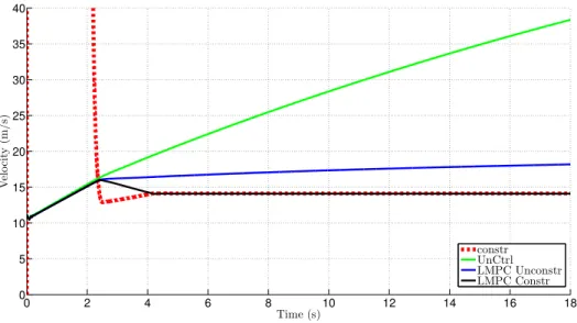
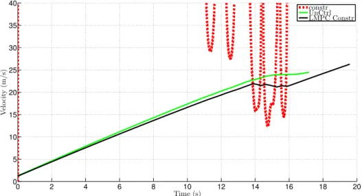
As shown in the velocity graph in Fig.4.1, the uncontrolled vehicle, green line, doesn’t regulate its speed during cornering whereas the controlled ones respond better. The blue line which corresponds to a vehicle similar to [30], has no hard constraint on both yaw rate and velocity although due to the constraining of the yaw rate reference signal we ob-serve a much better velocity reduction than the uncontrolled case. On the other hand, the controller implemented for this research adjusts the vehicle’s velocity quickly in less than 2 seconds and then remains constant during the maneuver slightly under the constraint. The soft constraint on the velocity allows the controller to find a solution even though the constraint itself is not respected, depending on the value of its weighting parameter inside the cost function, in our case the p_V in (3.2). All the details regarding the weights are mentioned in the Appendix section.

0 2 4 6 8 10 12 14 16 18 0 5 10 15 20 25 30 35 40 Time (s) V el o ci ty (m /s ) constr UnCtrl LMPC Unconstr LMPC Constr

4.1. SIMULATION RESULTS 41 Figure 4.2 shows the yaw rate responses of the three vehicles being compared. Once again, it is easily observed that the vehicle with equal torque split to all four wheels doesn’t go into a steady-state phase. The LMPC unconstrained vehicle has no hard con-straints on velocity as proved on the previous graph nor on yaw rate, but the yaw rate response has a lower slope and respects the yaw rate reference with a minor error. The only vehicle that goes into steady-state is the constrained LMPC. While there is a minor overshoot at the start of the step-steer between the seconds 2 and 3, which is allowed by the yaw rate soft constraint similar to the velocity one, the controller respects the yaw rate constraint quicker than the velocity case and then follows the reference signal with an error of 1.5°/s. Moreover, all the trajectories of the vehicles are shown in Fig.4.3 where

the fully constrained vehicle, LMPC Constr, completes a circle whereas the other vehicles are following a more spiral path.

0 2 4 6 8 10 12 14 16 18 −5 0 5 10 15 20 25 30 35 40 Time (s) Y aw R at e (d eg/s ) constr rrefLMPC Unconstr rrefLMPC Constr UnCtrl LMPC Unconstr LMPC Constr

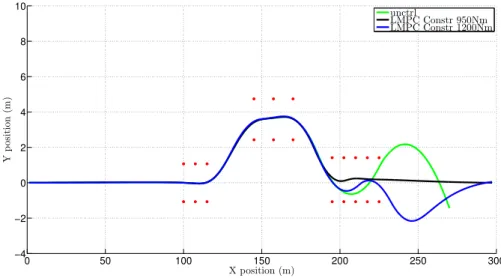
300 350 400 450 500 550 600 −20 0 20 40 60 80 100 120 140 160 180 X position (m) Y p os it ion (m ) unctrl LMPC Unconstr LMPC Constr

Figure 4.3: Position, step-steer atT_dmd =1000NmandVin=40k ph.

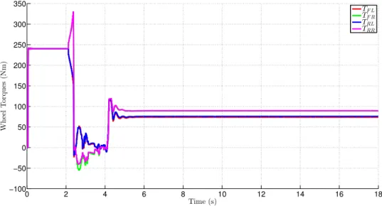
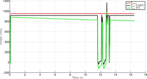
According to the system protection which all EVs have as mentioned in Chapter 3, the wheel torques of the same step-steer example (1000Nm and V_in = 40k ph) shown in Fig.4.4 don’t reach the expected 250Nm torque each, in the first 2 seconds due to the torque derates of the motor’s driving current limitations inside the system protection block. Furthermore after the 2 seconds have passed, we observe a torque reduction on the inner left wheels and a complementary increase on the outer right wheels of the vehicle, until the velocity constraint is hit where the vehicle starts braking. The braking torques are configured based on theq_Tdmd weighting parameter under the overspeeding case (see Appendix for further details). Under the chosen tuning parameters the controller brakes the outer wheels of the vehicle more than the inner ones trying to maintain stability and then enters the steady-state where all wheel torques are positive but the outer wheels have slightly more torque than the inner wheels.

Finally, to show the robustness of the controller working under a different range of driver’s torque demands, we observe on Fig.4.5 that all cases reach the steady-state. In this graph the dashed and continuous lines represent the driver’s torque demand and the

4.1. SIMULATION RESULTS 43 vehicle’s total torque respectively whereas the different line colors differentiate the sce-narios between them.

0 2 4 6 8 10 12 14 16 18 −100 −50 0 50 100 150 200 250 300 350 Time (s) W h ee l T or q u es (Nm ) TF L TF R TRL TRR

Figure 4.4: Wheel torques, step-steer atT_dmd=1000NmandV_in=40k ph.

0 2 4 6 8 10 12 14 16 18 −200 0 200 400 600 800 1000 1200 1400 1600 1800 Time (s) T or q u e (Nm ) Tdmd Ttot

4.1.1.2 Understeer gradient tuning performance

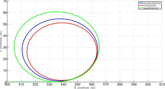
As shown in equation (3.3) theK_und has a crucial role on the yaw rate reference genera-tion. Having the ability to independently tune the understeer gradient of the controller’s internal vehicle model, gives us the freedom to extensively control the turning radius of the vehicle’s trajectory. The understeer gradient used for the tuning purposes is based on an understeer vehicle with K_und =0.0017rad/s=1°/g. Furthermore the robustness of the controller was tested for different values of K_und =0 andK_und =−0.0017rad/s

which correspond to a neutralsteer and oversteer vehicle respectively.

5000 510 520 530 540 550 560 570 580 590 600 610 10 20 30 40 50 60 70 X position (m) Y p os it ion (m ) neutralsteer oversteer understeer

Figure 4.6: Position responses of differentK_und, step-steer atT_dmd=1000NmandVin =

40k ph.

4.1.2

Double Lane Change

The double lane change maneuver we used is the ”Double Lane Change ISO” provided by CarMaker. The CarMaker driver parameters used for the lateral dynamics are shown in Fig.4.7 and the longitudinal dynamics are set manually through Simulink by the constant

4.1. SIMULATION RESULTS 45 driver’s torque demand. The vehicle was tested under different road friction coefficients assuming a constant torque demand from the driver and K_und =0.0017rad/sec, as as-sumed in the previous testing scenario also. One more important thing to mention is that our internal model has a configured constant road friction coefficientµ =0.7. This value

was chosen in order to test the controller’s robustness on a variety of different surfaces as it is demonstrated bellow.

Figure 4.7: Lateral dynamics CarMaker driver parameters.

4.1.2.1 Double Lane Changeµ =0.5

As we can see from both yaw rate and position figures, Fig.4.8 and Fig.4.9 respectively, the uncontrolled vehicle on low road friction coefficientµ =0.5 is starting to lose control

from a total torque demand of 700Nm and above whereas the LMPC can successfully complete the maneuver. However, the maximum torque demand on the LMPC is limited up to 720Nmbefore the controlled vehicle is unable to maintain stability for the given set of tuning parameters. Although this can be increased by changing the tuning parameters of the controller, the weights inside the cost function, appropriately.

because the driver is the one who controls the steering wheel which has a large effect on the excitement of the vehicles yaw rate. Although the controller continues to find an optimal solution as it is shown on later graphs, because of the soft constraints used as mentioned in Section 3. 0 2 4 6 8 10 12