Contents lists available atScienceDirect
Neural Networks
journal homepage:www.elsevier.com/locate/neunet
2015 Special Issue
Expected energy-based restricted Boltzmann machine
for classification
S. Elfwing
∗, E. Uchibe, K. Doya
Okinawa Institute of Science and Technology Graduate University, 1919-1 Tancha, Onna-son, Okinawa 904-0495, Japan
a r t i c l e i n f o
Article history:
Available online 28 September 2014
Keywords:
Classification
Restricted Boltzmann machine Expected energy
Free energy
a b s t r a c t
In classification tasks, restricted Boltzmann machines (RBMs) have predominantly been used in the first stage, either as feature extractors or to provide initialization of neural networks. In this study, we propose a discriminative learning approach to provide a self-contained RBM method for classification, inspired by free-energy based function approximation (FE-RBM), originally proposed for reinforcement learning. For classification, the FE-RBM method computes the output for an input vector and a class vector by the negative free energy of an RBM. Learning is achieved by stochastic gradient-descent using a mean-squared error training objective. In an earlier study, we demonstrated that the performance and the robustness of FE-RBM function approximation can be improved by scaling the free energy by a constant that is related to the size of network. In this study, we propose that the learning performance of RBM function approximation can be further improved by computing the output by the negative expected energy (EE-RBM), instead of the negative free energy. To create a deep learning architecture, we stack several RBMs on top of each other. We also connect the class nodes to all hidden layers to try to improve the performance even further. We validate the classification performance of EE-RBM using the MNIST data set and the NORB data set, achieving competitive performance compared with other classifiers such as standard neural networks, deep belief networks, classification RBMs, and support vector machines. The purpose of using the NORB data set is to demonstrate that EE-RBM with binary input nodes can achieve high performance in the continuous input domain.
©2014 The Authors. Published by Elsevier Ltd. This is an open access article under the CC BY-NC-ND license (http://creativecommons.org/licenses/by-nc-nd/3.0/).
1. Introduction
For classification tasks, restricted Boltzmann machines (RBMs)
(Freund & Haussler, 1992;Hinton,2002;Smolensky,1986) have
predominantly been used for generative learning in the first stage of the classification, either as feature extractors for other classi-fication algorithms or to provide weight initialization of neural network classifiers. Classification RBMs (classRBMs) (Hinton,
Osin-dero, & Teh, 2006;Larochelle & Bengio, 2008) were proposed to
provide a self-contained discriminative RBM framework for devel-oping competitive classifiers. ClassRBMs can be trained with a gen-erative learning objective (learning of the joint distributionP
(
x,
y)
of the input vectorxand the target vectory) and/or a discrimi-native learning objective (learning of the conditional distribution
P
(
y|
x)
directly). As noted byLarochelle, Mandel, Pascanu, and Ben-gio(2012), a discriminative learning approach offers two advan-tages for classification compared with generative RBM learning for∗Corresponding author. Tel.: +81 989668594.
E-mail addresses:[email protected](S. Elfwing),[email protected](E. Uchibe), [email protected](K. Doya).
feature extraction: (1) it requires no additional training phase of a separate classifier, which makes it possible to track the classifi-cation performance on a validation set and (2) it facilitates model selection, based on validation set performance, because no addi-tional meta-parameters of the separate classifier must be tuned. The use of RBMs for weight initialization or pretraining of deep neural networks (seeHinton et al.,2006;Salakhutdinov & Hinton, 2009, for instance) shares the same disadvantages since it requires two training phases. Another discriminative RBM approach was proposed bySchmah, Hinton, Zemel, Small, and Strother(2008). They trained a separate RBM for each class and classification was determined by the free energy of each network.
In this study, we propose an alternative discriminative learning approach to provide a self-contained discriminative RBM method for classification. It is inspired by free-energy based function approximation, originally proposed bySallans and Hinton(2004) for reinforcement learning (hereafter,FE-RBM). For classification, the FE-RBM method computes the output,Q, for an input vector
xand a class vectoryby the negative free energy,F, of an RBM:
Q
= −F
= −⟨E⟩ +
H, where⟨E⟩
is the expected energy andHis the entropy of the network. Learning in the FE-RBM method
http://dx.doi.org/10.1016/j.neunet.2014.09.006
0893-6080/©2014 The Authors. Published by Elsevier Ltd. This is an open access article under the CC BY-NC-ND license (http://creativecommons.org/licenses/by-nc-nd/3. 0/).
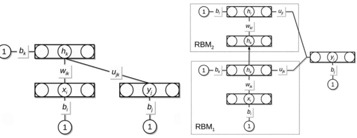
Fig. 1. The RBM architecture (left panel) and a stacked RBM architecture with two RBMs and connections to the class nodes from the hidden layer of both RBMs (right panel). In the stacked architecture, the hidden activations are computed layer-by-layer in a bottom-up fashion. The hidden activations of the first RBM serve as a fixed input vector to the second RBM.
is achieved by stochastic gradient-descent using a mean-squared error training objective.
In our earlier work (Elfwing, Uchibe, & Doya, 2013), we showed that the robustness and learning performance of FE-RBM can be improved by scaling the free energy by a constant scaling factor,
Z, to ensure that the outputs are initialized within an appropriate range. In this study, we propose that the learning performance of RBM function approximation can be further improved by computing the output by the negative expected energy, instead of the negative free energy, i.e.,Q
= −⟨E⟩
(hereafter,EE-RBM).Our approach is probably more closely related to standard neu-ral networks than traditional RBM approaches for classification. Like standard neural network learning, the EE-RBM method learns the target value for each class using stochastic gradient-descent with a mean-squared error learning objective. Unlike neural networks, the output is not computed in specific output nodes. Instead, the output is computed as the weighted sum of all bi-directional connections in the network (i.e., the negative expected energy), where the class vector has an ‘‘one-out-of-J’’ representa-tion and funcrepresenta-tions as a fixed input to the network.
To create a deep learning architecture, we stack several RBMs on top of each other. We also connect the class nodes to all hidden layers to try to improve the performance even further. This approach has previously been utilized by deep energy models
(Ngiam, Chen, Koh, & Ng, 2011) and Raiko, Valpola, and LeCun
(2012) connected every other hidden layer to the output nodes in multilayer neural networks. In the deep architectures, we define the outputQ for EE-RBM as the sum of the negative expected energy over all stacked RBMs.
We validate the classification performance of our proposed method using the MNIST and NORB data sets. It is a common obser-vation that, for generative learning, RBMs with binary input nodes are only well-suited for domains with binary or strongly bimodal input values, such as the MNIST data set (seeHinton,2010;Nair &
Hinton, 2008, for instance). For tasks with continuous inputs, such
as the grayscale images in the NORB data set, RBM methods with Gaussian input nodes have been applied successfully (seeHinton
& Salakhutdinov, 2006;Nair & Hinton, 2008;Salakhutdinov &
Hin-ton, 2009, for instance).Bengio, Lamblin, Popovici, and Larochelle
(2006) demonstrated a 12 percentage points improvement in clas-sification performance for deep belief networks with Gaussian in-put nodes compared with binomial inin-put nodes, for a financial data set with real-valued inputs. The purpose of using the NORB data set is to demonstrate that EE-RBM with simple binary input nodes can achieve high classification performance in the continuous in-put domain.
2. Method
2.1. FE-RBM for classification
The classification method we propose in this study is inspired
bySallans and Hinton(2004), where they introduced the use of an
RBM as a function approximator in reinforcement learning (Sutton
& Barto, 1998). In a classification context, the structure of the
network is the same as for the classRBM; see the left panel in
Fig. 1. The RBM consists of binary input nodes,x, class nodes,y, and
hidden nodes,h. Theith input node,xi, is connected tokth hidden nodehkby the weight
wik
, and thejth class node,yj, is connected to thekth hidden nodehkby the weightujk. In addition, the input nodes, the class nodes, and the hidden nodes are all connected to a constant bias input with a value of 1, with connection weightsbi
,
bj, andbk, respectively. The class vectoryhas an ‘‘one-out-of-J’’ representation and functions as a fixed input to the network for each class. Letyjdenote the vector for classj, whereyjis equal to one and the rest of the class nodes are equal to zero. The energy,E, of the RBM for input vectorxand class vectoryjis given byE
(
x,
yj,h)
= −
K
k=1 I
i=1 xiwikhk−
K
k=1 J
j∗=1 yj∗uj∗khk−
I
i=1 bixi−
J
j∗=1 bj∗yj∗−
K
k=1 bkhk (1)= −
K
k=1 I
i=1 xiwikhk−
K
k=1 ujkhk−
I
i=1 bixi−
bj−
K
k=1 bkhk. (2)Here,I is the number of input nodes,J is the number of classes, and K is the number of hidden nodes. The free energy,F, can be computed as the sum of the expected energy,
⟨E⟩
, and the negative entropy,H, where the expectations are taken with respect to the posterior distribution of the hidden values,P(
h|
x,
yj). The expected hidden activation (i.e., the probability that the hidden value is equal to one) of hidden nodekfor classj,
⟨h
jk⟩
, is given by⟨h
jk⟩ =
P(
hk=
1|
x,
yj)=
σ
I
i=1 xiwik+
ujk+
bk
,
σ (
x)
=
1 1+
e−x.
(3)The free energy is then given as F
(
x,
yj)= ⟨E
(
x,
yj,h)
⟩ +
−H(x,yj)
⟨
logP(
h|
x,
yj)⟩
(4)= −
K
k=1 I
i=1 xiwik⟨h
jk⟩ −
K
k=1 ujk⟨h
jk⟩
−
I
i=1 bixi−
bj−
K
k=1 bk⟨h
jk⟩
+
K
k=1
⟨h
jk⟩
log⟨h
jk⟩ +
(
1− ⟨h
jk⟩
)
log(
1− ⟨h
jk⟩
)
.
(5) For classification, the FE-RBM method computes the outputQfor an input vectorxand a class vectoryj by the negative free energy,
−F
, of the network:Q
(
x,
yj)= −F
(
x,
yj)= −⟨E
(
x,
yj,h)
⟩ +
H(
x,
yj). (6) Lettdenote the target vector, which is equal to the class vectorycorresponding to the correct classification of the current training example, i.e., the target value is one for correct classification and zero otherwise. The stochastic gradient-descent update of the parameters,
θ
, of theQ-function for a mean-squared error training objective is then computed byθ
←
θ
+
α
J
j=1
tj−
Q(
x,
yj)
∇
θQ(
x,
yj). (7)Here,
α
is the learning rate.Classification of input vectors with unknown class labelsjin validation and test sets are made according to the largest output:
j
=
arg max iQ
(
x,
yi). (8)For FE-RBM, the derivatives of theQ-function with respect to the network parameters (
wik,
ujk,bi,
bj, andbk) are computed by∇
wikQ(
x,
yj)=
xi⟨h
jk⟩
,
(9)∇
ujkQ(
x,
yj)=
yj⟨h
jk⟩
,
(10)∇
biQ(
x,
yj)=
xi, (11)∇
bjQ(
x,
yj)=
yj, (12)∇
bkQ(
x,
yj)= ⟨h
jk⟩
.
(13)2.2. EE-RBM for classification
In our earlier work (Elfwing et al., 2013), we demonstrated that the robustness and the learning performance of RBM function approximation can be improved by scaling the free energy by constant scaling factor,Z, that is related to the size of the network. By setting the scaling factor to a large enough value, the output can be initialized within an appropriate range, i.e., smaller than the maximum target value of 1. In this study, we propose that RBM function approximation for classification can be further improved by computingQ by the negative expected energy, instead of the negative free energy:
Q
(
x,
yj)= −⟨E
(
x,
yj,h)
⟩
.
(14)For EE-RBM, an additional term:
⟨h
jk⟩
(
1− ⟨h
jk⟩
)
zkj, (15)is added to the derivative expressions with respect to the network parameters
wik,
ujk, andbk(Eqs.(9),(10), and(13), respectively).Here,zkjis the input to the hidden sigmoid activation function of hidden nodekfor classj(Eq.(3)):
zkj
=
I
i=1
xiwik
+
ujk+
bk. (16)For example, for EE-RBM, the derivatives of theQ-function with respect to
wik
is changed to∇
wikQ(
x,
yj)=
xi
⟨h
jk⟩ + ⟨h
jk⟩
(
1− ⟨h
jk⟩
)
zkj
.
(17)This derivative expression is derived in theAppendix.
2.3. Stacked RBMs
To create a deep learning network structure, we stack several RBMs on top of each other and connect the class nodes to the hid-den layers of all the stacked RBMs; see the right panel inFig. 1for an illustration of a network with two stacked RBMs. The expected hid-den activation is computed layer-by-layer in a bottom-up fashion. The expected hidden activations of the first RBM serve as a fixed input vector for the computations of the expected hidden activa-tions of the second RBM, and so on. For the first RBM, the expected hidden activations,
⟨h
jk⟩
, are therefore computed according to Eq. (3), and the free energy,FRBM1, and the expected energy,⟨E⟩
RBM1, are computed according to Eq.(5). For the second RBM, expected hidden activations,⟨h
jl⟩
, are computed by⟨h
jl⟩ =
σ
K
i=1⟨h
jk⟩
wkl
+
ujl+
bl
.
(18)Here, the weight
wkl
is connecting hidden nodekin the first RBM and hidden nodelin the second RBM, the weightujlis connecting class nodejand hidden nodel, andblis the bias weight for hidden nodel. The expected energy of the second RBM,⟨E⟩
RBM2, is com-puted by⟨E⟩
RBM2= −
L
l=1 K
k=1⟨h
jk⟩
wkl
⟨h
jl⟩ −
L
l=1 ujl⟨h
jl⟩ −
L
l=1 bl⟨h
jl⟩
,
(19) and the entropy,HRBM1is computed byHRBM2
= −
L
l=1
⟨h
jl⟩
log⟨h
jl⟩ +
(
1− ⟨h
jl⟩
)
log(
1− ⟨h
jl⟩
)
.
(20) For the stacked RBM architecture, we define theQ-function as the sum of the negative free energy (Q=
i
−F
RBMi) and the sum of negative expected energy (Q=
i
−⟨E⟩
RBMi) over all RBMs in the stack, for FE-RBM and EE-RBM, respectively. For an architecture with two RBMs, the FE-RBM derivatives of the Q-function with respect towkl
andwik
are computed by∇
wklQ(
x,
yj)= ⟨h
jk⟩⟨h
jl⟩
,
(21)∇
wikQ(
x,
yj)=
xi
⟨h
jk⟩ +
(
1− ⟨h
jk⟩
)
L
l=1wkl
∇
wklQ(
x,
yj)
,
(22) and the EE-RBM derivatives are computed by∇
wklQ(
x,
yj)= ⟨h
jk⟩
⟨h
jl⟩ + ⟨h
jl⟩
(
1− ⟨h
jl⟩
)
zlj
,
(23)∇
wikQ(
x,
yj)=
xi
⟨h
jk⟩ + ⟨h
jk⟩
(
1− ⟨h
jk⟩
)
zkj+
(
1− ⟨h
jk⟩
)
L
l=1wkl
∇
wklQ(
x,
yj)
.
(24)Here,zljis the input to the hidden sigmoid activation function of hidden nodelin the second RBM for classj(Eq.(18)):
zlj
=
k
k=1⟨h
jk⟩
wkl
+
ujl+
bl.
(25) 2.4. InitializationIn our experience, to achieve robust and efficient learning, the amplitude of the random initialization of the weights between the class nodes and the hidden nodes (ujkand ujl) has to be several magnitudes larger than the amplitude of the random initialization of the other weights. This means that if the weights are randomly initialized using a distribution with zero mean, then the initialQ -function for both FE-RBM and EE-RBM will grow with the number of hidden nodes, with a faster rate for FE-RBM (see the left panel
inFig. 9). To ensure that the initial outputQ
≈
0.
5, we used thescaling technique we proposed inElfwing et al.(2013), by settingZ
to approximately twice the initialQwithout scaling. In our earlier study, we also showed that scaling theQ-function byZis equiv-alent to multiply the target value byZand re-scaling the learning rate (
α
′=
α/
Z2). In this study, we follow this approach (for bothFE-RM and EE-RBM) by setting the target value for correct classifi-cation toZ, instead of one.
3. Experiments
3.1. MNIST handwritten digit data set
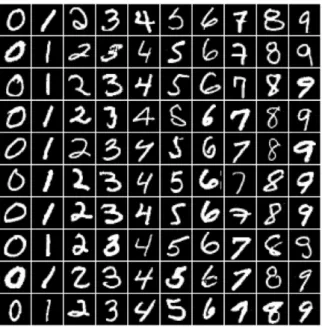
The MNIST data set (LeCun, Bottou, Bengio, & Haffner, 1998) consists of 60 000 training images and 10 000 test images of ten handwritten digits, zero to nine, with an image size of 28
×
28 pixels (seeFig. 2for example images), i.e., the dimension of the input vector was 784. The grayscale pixel values were normalized to the range[
0;
1]
by dividing the values by 255.3.1.1. Shallow networks
In the first set of experiments, we used shallow networks with 800 nodes in the hidden layer. To evaluate EE-RBM and FE-RBM, we compared the performance with a standard feedforward neural network (NN) and a discriminative classRBM network, also with 800 nodes in the hidden layer. For the neural network, we used sigmoid activation functions for both the hidden and the output nodes, and the learning was achieved by stochastic gradient-descent with a mean-squared error training objective. For the discriminative classRBM network, p
(
yj|
x)
can be computed byLarochelle et al.(2012) p
(
yj|
x)
=
exp
bj+
k log(
1+
exp(
zkj))
j∗∈{1,...,J} exp
bj∗+
k log(
1+
exp(
zkj∗))
.
(26)For the training objective
−
logp(
yj|
x)
, the gradient for the class node biases can be computed by∂
logp(
yj|
x)
∂
bj=
tj−
p(
yj|
x),
(27)and the gradient for
wik,
ujk, andbkcan be computed by∂
logp(
yj|
x)
∂θ
=
k⟨h
jk⟩
∂
zkj∂θ
−
k,j∗⟨h
jk∗⟩p
(
yj∗|
x)
∂
zkj∗∂θ
.
(28)Fig. 2. Example images of the ten handwritten digits in the MNIST training set.
Following the experimental setup inLarochelle et al.(2012), we randomly separated the original training set into a training set of 50 000 images and a validation set of 10 000 images, and used the original test set of 10 000 images. For each method, we used a grid-like search to determine the learning rate
α
(between 0.005 and 0.1, on a log scale, for NN and classRBM, and between 0.
005/
Kand 0.
1/
Kfor FE-RBM and EE-RBM) based on the performance on the validation set. The stopping criteria, i.e., the number of learning epochs (iterations over the training set) for each experiment, were also determined by the performance on the validation set, with a look ahead of 15 epochs. For NN and classRBM, the weight matrices were randomly initialized using a uniform distribution with values between−m
−0.5and m−0.5, wheremwas the maximum of thenumber of rows and columns of the matrices. The bias weights in the classRBM networks were initialized to zero. For FE-RBM and EE-RBM, theujkweights were randomly initialized using a uniform distribution with values between
−
1.5 and 1.5. All other weights were randomly initialized using a uniform distribution with values between−
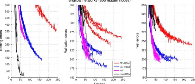
0.001 and 0.001.After determining the appropriate learning rates, we used four additional random separations of the original training set into a training set and a validation set to evaluate the performance of each method.Fig. 3shows the errors on the training set (left panel) and the validation set (middle panel) during learning for the five experiments for each of the four methods. To be able to observe the variance in classification performance, we also checked the number of errors on the test set after each epoch of learning on the training set (right panel). The best and the mean performances on the test set (as well as the learning rates and the average number of learning epochs) are summarized in the first part ofTable 1.
Although the discriminative classRBM networks achieved the fastest learning and the best performance on the training set, the performance on the test set was significantly worse compared with the other types of networks. The classRBM networks also had the largest variance in classification performance on the test set. The difference between the mean performance and the best performance was about 35 test errors, compared to about 10 test errors for the other types of networks. NN and EE-RBM achieved almost identical performance on the test set, 200.2 test errors in average for both methods and best performances of 192 test errors for EE-RBM and 191 test errors for NN. The performance achieved by FE-RBM was about 50 test errors worse than performance achieved by NN and EE-RBM.
Fig. 3. The number of errors on the training set (left panel), validation set (middle panel), and test set (right panel) for MNIST experiments with shallow networks with 800 hidden nodes. The length of the each of the five experiments for each method was determined by the validation set performance with a 15 steps look ahead.
Table 1
Comparison of classification results on the MNIST data set, as well as the average number of training epochs and determined learning rates.
α Epochs Test errors Mean Mean Best Shallow networks: 800 hidden nodes
FE-RBM 0.01/K 188.0 249.6 241
EE-RBM 0.01/K 141.2 200.2 192
NN 0.05 84.8 200.2 191
classRBM 0.05 57.0 315 279
Deep networks: 800–800 hidden nodes
FE-RBM fully connected 0.01/(K+L) 73.4 204.0 189 FE-RBM top connected 0.01/(K+L) 88.0 206.6 186 EE-RBM fully connected 0.01/(K+L) 43.2 141.2 133 EE-RBM top connected 0.01/(K+L) 89.0 172.0 163
NN 0.05 126.0 214.8 197
Deep networks: 2000–2000 hidden nodes
EE-RBM fully connected (training set: 50k) 0.01/(K+L) 26.3 127.3 119 EE-RBM fully connected (training set: 60k) 0.01/(K+L) 26 107
3.1.2. Deep networks
In the second set of experiment, we used a stacked RBM archi-tecture with two RBMs and 800 hidden nodes in both RBMs. We compared the performance with a neural network with two hid-den layers, also with 800 nodes in both hidhid-den layers. To investi-gate the benefit of connecting the class nodes to both hidden layers, we performed additional experiments where the class nodes were only connected to the hidden layer of the top (second) RBM, i.e. the connection weightsujk(see the right panel inFig. 1) were removed. Hereafter,top connecteddenotes networks where the class nodes are only connected to the hidden layer of the top RBM andfully connecteddenotes networks where the class nodes are connected to the hidden layers in all RBMs. We used the same procedure as in the earlier experiments to create the training and validation sets, determine the learning rate
α
(the search range forα
was changed to between 0.
005/(
K+
L)
and 0.
1/(
K+
L)
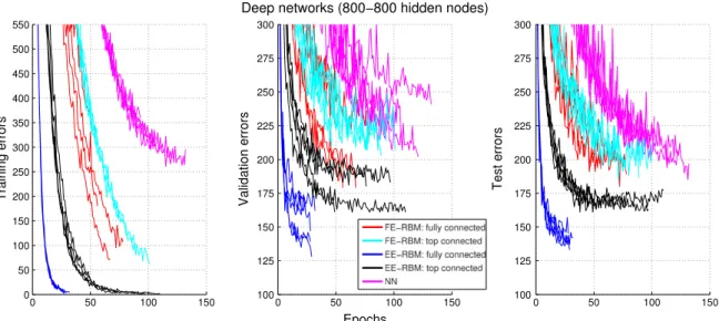
for FE-RBM and EE-RBM), and determine the number of learning epochs.The experimental results are visualized inFig. 4and the per-formances on the test set are summarized in the second part of
Table 1. The addition of a second hidden layer did not improve
the performance of NN. Instead, the average number of test errors increased by about 15 and the learning time increased by about 40 epochs. For FE-RBM, the addition of a second RBM improved
the mean performance by 45 test errors to about 205 test errors, i.e., slightly worse than the performance of the shallow NN and EE-RBM networks. It also cut the learning time in half compared with the shallow FE-RBM networks. There was no notable difference in performance between the fully connected and the top connected networks, except for a slight decrease in the learning time for the fully connected networks. In contrast, the mean performance of 141.2 achieved by the fully connected EE-RBM networks was an improvement by about 30 test errors compared with the top con-nected EE-RBM networks, and it was achieved in less than half the learning time. The fully connected EE-RBM networks also showed the largest increase in performance by adding a second RBM. Com-pared with the shallow EE-RBM networks, the classification per-formance improved by about 60 test errors and the learning time decreased by more than three times.
In the third set of experiment, we investigated the effect on the performance for the fully connected EE-RBM network of increasing the number of nodes in the hidden layers to 2000 for both RBMs. For the larger network, we performed experiments on three differ-ent random separations of the original training set into training and validation sets. In addition, we performed an experiment in which we used the original training set of 60 000 images to train the net-work. As stopping criteria, we used the average learning time (26
Fig. 4. The number of errors on the training set (left panel), validation set (middle panel), and test set (right panel) for MNIST experiments with deep networks with 800 nodes in both hidden layers. The length of the each of the five experiments for each method was determined by the validation set performance with a 15 steps look ahead.
Fig. 5. The number of errors on the training set (left panel), validation set (middle panel), and test set (right panel) for MNIST experiments with deep networks with 20 000 nodes in both hidden layer.
epochs) determined by the performance on the validation set in the three experiments trained on the smaller training set of 50 000 images. The experimental results are visualized inFig. 5and the performances on the test set are summarized in the third part of
Table 1. The increase of the number of hidden nodes to 2000
im-proved the classification performance with about 14 test errors to a mean performance of 127.3 test errors and a best performance of 119 test errors. The mean learning time was also reduced by about 17 epochs to 26.3 epochs. By using the original training set, the classification performance was further improved to 107 test errors.
3.2. NORB object image data set
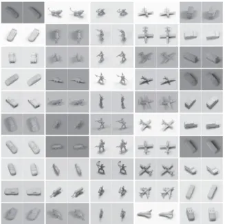
The NORB data set (LeCun, Huang, & Bottou, 2004) consists of grayscale stereo images of 50 toys belonging to 5 generic classes: cars, four-legged animals, human figures, airplanes, and trucks (see
Fig. 6for example stereo images). Different images capture the
objects from different points of view and under different lighting conditions. The training set consists of 24 300 stereo images of 25 objects (5 objects and 4860 images for each class). The test set consists of 24 300 stereo images of the other 25 objects, i.e., there
is no overlap between the training set and the test set. The size of each stereo image is 96
×
96 pixels, i.e., the dimension of the input vector was 96×
96×
2=
18 432. The grayscale pixel values were normalized to the range[
0;
1]
by dividing the values by 255.In the more difficult NORB task, the learning rate
α
was set to 0.
0001/(
K+
L)
, i.e., two magnitudes smaller than in the MNIST task. For larger values ofα
, the learning converged very early on to suboptimal solutions where all training examples were classified to belong to one or two classes. The class weights ujk and ukl were randomly initialized using a uniform distribution with values between−
2 and 2. All other weights were randomly initialized using a uniform distribution with values between−
0.001 and 0.001.For the NORB task, we trained a fully connected FE-RBM net-work and a fully connected EE-RBM netnet-work with two RBMs and 2000 nodes in both hidden layers. We confirmed that FE-RBM with binary input nodes is unsuitable in the continuous input domain.
Fig. 7shows the misclassification rate on the training set and the
misclassification rate on the test set after each of the 200 epochs of learning. FE-RBM achieved a best performance of approximately 35% on the training set and 30% on the test set. However, there were
Fig. 6. Examples of stereo images of the five toy objects in the NORB training set.
Fig. 7. The misclassification rate on the training set and the misclassification rate on the test set after each epoch of learning in the NORB experiment for a fully connected FE-RBM network with two RBMs and 2000 nodes in both hidden layers.
very large, up to 20 percentage points, fluctuations in test set per-formance between epochs.
Instead of using a validation set, we trained the EE-RBM net-work on the full training set until the misclassification rate on the training set was exactly 0%.Fig. 8shows the misclassification rate on the training set (left panel) and the test set (right panel) after each epoch of learning. The misclassification rate on the training set reached 1% after about 50 epochs and converged to exactly 0% after 207 epochs. After the end of learning, the misclassification rate on the test set was 10.7%.
4. Analysis of the difference between expected energy and free energy function approximation
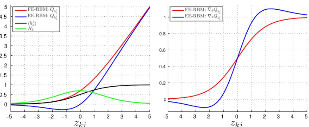
4.1. Hidden node output contributions and derivative functions
In this section, we analyze the difference between free energy and expected energy function approximation.Fig. 9visualizes the differences in function approximation between FE-RBM (red) and EE-RBM (blue). The left panel shows the contributions to theQ -function from hidden nodek
,
Qhjk
, as functions ofzkj, as well as
⟨h
jk⟩
(black) and the entropy for hidden nodek,
Hk(green). The contri-butions to theQ-function for EE-RBM (−⟨E⟩
hjk) and FE-RBM (
−F
hjk) can be computed by−⟨E⟩
hjk=
i xiwik⟨h
jk⟩ +
ujk⟨h
jk⟩ +
bk⟨h
jk⟩ = ⟨h
j k⟩z
kj, (29)−F
hjk= ⟨h
j k⟩z
kj−
⟨h
jk⟩
log⟨h
jk⟩ +
(
1− ⟨h
jk⟩
)
log(
1− ⟨h
jk⟩
)
Hk.
(30) For FE-RBM, theQhjk-function is a monotonically increasing non-negative function that is approximately equal to the sigmoid function forzkj-values smaller than approximately
−
2 and approx-imately equal tozkjfor large positivezkj-values. The computation of the outputQ for FE-RBM can be reformulated asQ
(
x,
yj)=
−
k Fhj k
+
i bixi+
bj
.
(31)This explains why FE-RBM cannot handle problems with contin-uous input, because the network has to counterbalance a sum of non-negative and non-linear functions
−
kFhjk
with a linear
Fig. 8. The misclassification rate on the training set (left panel) and the misclassification rate on the test set after each epoch of learning (right panel) in the NORB experiment for a fully connected EE-RBM network with two RBMs and 2000 nodes in both hidden layers.
Fig. 9. Visualization of FE-RBM (red) and EE-RBM (blue) function approximation. The left panel shows the contributions to theQ-function from hidden nodek,Qhj k
, as functions ofzkj, as well as⟨hjk⟩(black) and the entropy for hidden nodek,Hk(green). The right panel shows the derivative functions as functions ofzkj. (For interpretation of
the references to color in this figure legend, the reader is referred to the web version of this article.)
function
ibixi+
bj
. In the case of binary input, this problem is much less severe, because the weighted inputs,xiwik, to a hidden nodekhave only two possible values: 0 (xi
=
0) orwik
(
xi=
1)
. In-terestingly, for EE-RBM, theQhjk
-function is not monotonically in-creasing and not non-negative. Instead, it has a global minimum value of approximately
−
0.28 forzkj≈ −
1.
28.The right panel inFig. 9shows the derivative functions for FE-RBM and EE-FE-RBM with respect toujk,bk, and
wik
(for active input nodesxi), assuming that the input vector is binary. For FE-RBM, the derivative function is equal to the monotonically increasing sigmoid function. For EE-RBM, the derivative function has two extreme values. It ‘‘undershoots’’ zero forzkjapproximately smaller than−
1.28 (corresponding to the minimum of−⟨E⟩
hjk) and it ‘‘overshoots’’ one forzkjapproximately larger than 1.28, and then it asymptotically approaches zero and one forzkj
→ −∞
andzkj
→ ∞
, respectively. The derivative function has a maximum value of approximately 1.1 and a minimum value of approximately−
0.1 forzkj≈ ±
2.
4, i.e., the solutions to the equation−z
kj=
log
(
zkj−
2)/(
zkj+
2)
. This suggest that for EE-RBM there is ‘‘soft floor’’ atzkj
≈ −
1.
28, which serves as an implicit weight regularizer.4.2. Trained weights
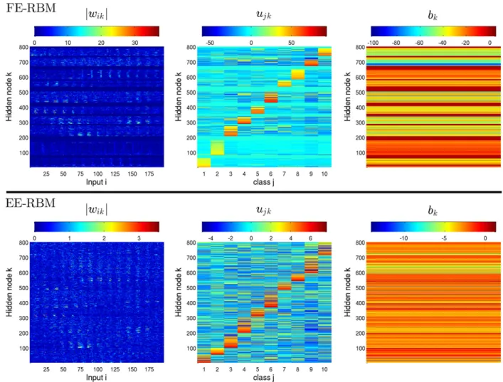
To investigate the difference between the two methods further, we looked at the trained weights for the best shallow networks used in the MNIST task.Fig. 10shows the magnitudes of
wik
(left panels), and the actual values ofujk(middle panels), andbk(right panels). The hidden nodes were sorted according to the magnitude ofujkand grouped according to classj. The visualized data shows three obvious differences between the two methods. First, the ranges of the trained FE-RBM weights (top panels) were about a magnitude larger than the EE-RBM weights (bottom panels). This gives support to the hypothesis above that the ‘‘soft floor’’ atzkj≈
−
1.
28, where the derivative function is zero, plays an important regularizing role in EE-RBM learning, by preventing the learning of weights with large magnitudes. Second, the trained FE-RBM network had a much less shared (or less global) weight structure. Most of the hidden nodes only had connections with one or a few class nodes with larger positive weights (top middle panel). The weights of the other class connections were, typically, either close to zero or had values of about−
10. This means that the output for the different classes was to a large extent determined by non-overlapping subsets of the hidden nodes. Third, for about 20% of the hidden nodes in the FE-RBM network, the connections weights to all other nodes were close to zero with small negative bias (see the dark blue, cyan, and dark red colored bands in the left, middle, andright top panels, respectively). Those hidden nodes were therefore not used in the feature extraction and contributed approximately zero to the output. We confirmed this by computing
−F
hjk of the non-contributing hidden nodes (173) for 100 images in the test set for each class. For all images and all classes, the total contribution
−
kFhjk
to theQ-function was less than 0.1% of the maximum target value.
5. Discussion
In this study, we proposed a discriminative learning approach, EE-RBM, to provide a self-contained RBM method for classification. The output of an EE-RBM network is computed by the negative expected energy (i.e., the weighted sum of all bi-directional connections in the network) and trained by standard stochastic gradient-descent with a mean-squared error learning objective. To create a deep learning structure we stacked several RBMs on top of each other and connected the class nodes to the hidden layers of all RBMs. EE-RBM networks achieved both fast and high classification performance on the MNIST and NORB data sets. The experiments clearly showed that the performance of EE-RBM increased significantly (approximately 30 test errors for 800–800 networks) when the class nodes were connected to all hidden layers. In contrast, for FE-RBM, there was no difference in performance between fully connected and top connected networks.
The result on the MNIST data set of on average 127 (best perfor-mance of 119) test errors using 50 000 training images and 107 test errors using 60 000 training images is competitive compared with the reported results of other discriminative ‘‘black box’’ classifiers such as the approximately 140 test errors achieved by support vec-tor machines (Decoste & Schölkopf, 2002), 160 test errors achieved by standard NNs (Hinton, Srivastava, Krizhevsky, Sutskever, &
Salakhutdinov, 2012), and the 181 test errors achieved by
discrim-inative classRBMs (Larochelle & Bengio, 2008). The result achieved by classRBM was improved to 128 test errors when using a hybrid training objective with tuned weighting of the two objectives, and further improved to 116 test errors with the introduction of an ex-tra parameter to encourage sparsity in the hidden layer.
Compared with the reported results for comparable deep RBM learning approaches, the result achieved by EE-RBM is competitive compared with deep belief networks and it is basically the same as for a deep neural network initialized using RBMs. Using the first approach,Hinton et al.(2006) achieved 139 test errors after 300 epochs using 50 000 training images and 125 test errors when the training was extended for 59 epochs using all 60 000 training images. Using the second approach, Hinton (2007) achieved a mean performance of 121 (best performance of 116) test errors
Fig. 10. The magnitudes ofwik(left panels), and the actual values ofujk(middle panels), andbk(right panels). Note that the figure only shows the 196wik-weights connected
to image pixels in the 14×14 center part of the images. (For interpretation of the references to color in this figure legend, the reader is referred to the web version of this article.)
after 51 epochs using 50 000 training images and 112 (best performance of 106) test errors when the training was extended for 25 epochs using all 60 000 training images.
The result on the NORB data set of a misclassification rate of 10.7% achieved by EE-RBM is similar to the 10.6% and the 10.8% achieved by the multi-prediction deep Boltzmann machine (
Good-fellow, Mirza, Courville, & Bengio, 2013) and the deep Boltzmann
machine (Salakhutdinov & Hinton, 2009), respectively, both with Gaussian input nodes, slightly better than the 11.6% achieved by support vector machines (Bengio & LeCun, 2007), and better than the 18.4% achieved by theK-nearest neighbors (LeCun et al., 2004) and 22.5% achieved by logistic regression (Salakhutdinov &
Hin-ton, 2009). It is noteworthy that EE-RBM with binary input nodes
achieved high performance on the NORB data set. To our knowl-edge, there is no reported result of high classification performance achieved by generative RBM approaches (or the discriminative FE-RBM method in this study) using binary input nodes in a continu-ous input domain.
It is encouraging that the results were achieved using standard stochastic gradient-descent learning and a fixed learning rate. The achieved results by EE-RBM are impressive compared with the state-of-the-art for the MNIST and NORB data sets. For both data sets, the performance can be significantly improved by exploiting knowledge about spatial structures by convolutional neural networks (LeCun et al., 1998) and further improved by augmenting the training set with transformations of the original set of the images (Cireşan, Meier, Gambardella, & Schmidhuber, 2010). In addition, the recently proposed dropout training technique
(i.e., random exclusion of input and hidden nodes during training,
seeHinton et al., 2012) has been shown to significantly improve
performance. For example, the performance of standard NNs on the MNIST data set was improved from 160 to about 110 test errors. For the permutation invariant versions of the two data sets, to our knowledge, the EE-RBM performance of 10.7% on the NORB data set and 107 test errors on the MNIST data set are the best reported results that neither used regularization by modeling the input distribution nor dropout training (see, Table 1 inGoodfellow,
Warde-Farley, Mirza, Courville, & Bengio, 2013, for results on the
MNIST data set).
Acknowledgment
This work was supported by Grant-in-Aid for Scientific Re-search on Innovative Areas: Prediction and Decision Making 23120007 and 26120727.
Appendix
In this appendix, we derive the derivative of theQ-function with respect to weights
wik
for EE-RBM (Eq.(17)):∂
Q∂wik
=
∂
∂wik
K
k=1 I
i=1 xiwik⟨h
jk⟩ +
K
k=1 ujk⟨h
jk⟩
+
I
i=1 bixi+
bj+
K
k=1 bk⟨h
jk⟩
(A.1)=
xi⟨h
jk⟩ +
∂
⟨h
jk⟩
∂wik
I
i=1 xiwik
+
∂
⟨h
jk⟩
∂wik
ujk+
∂
⟨h
jk⟩
∂wik
bk (A.2)=
xi⟨h
jk⟩ +
∂
⟨h
jk⟩
∂wik
zkj,see Eq.(16)
I
i=1 xiwik
+
ujk+
bk
(A.3)=
xi⟨h
jk⟩ + ⟨h
j k⟩
(
1− ⟨h
j k⟩
)
xizkj (A.4)=
xi
⟨h
jk⟩ + ⟨h
jk⟩
(
1− ⟨h
jk⟩
)
zkj
.
(A.5) ReferencesBengio, Y., Lamblin, P., Popovici, D., & Larochelle, H. (2006). Greedy layer-wise training of deep networks. InProceedings of advances in neural information processing systems (NIPS2006). Vol. 19.
Bengio, Y., & LeCun, Y.(2007). Scaling learning algorithms towards AI. InLarge scale kernel machines. MIT Press.
Cireşan, D. C., Meier, U., Gambardella, L. M., & Schmidhuber, J.(2010). Deep, big, simple neural nets for handwritten digit recognition.Neural Computation, 22(12), 3207–3220.
Decoste, D., & Schölkopf, B.(2002). Training invariant support vector machines. Machine Learning,46(1–3), 161–190.
Elfwing, S., Uchibe, E., & Doya, K.(2013). Scaled free-energy based reinforcement learning for robust and efficient learning in high-dimensional state spaces. Frontiers in Neurorobotics,7(3).
Freund, Y., & Haussler, D.(1992). Unsupervised learning of distributions on binary vectors using two layer networks. InAdvances in neural information processing systems, Vol. 4.
Goodfellow, I. J., Mirza, M., Courville, A., & Bengio, Y. (2013). Multi-prediction deep Boltzmann machines. InProceedings of advances in neural information processing systems (NIPS2013). Vol. 26.
Goodfellow, I. J., Warde-Farley, D., Mirza, M., Courville, A., & Bengio, Y. (2013). Maxout networks. InProceedings of the international conference on machine learning (ICML2013).
Hinton, G. E. (2002). Training products of experts by minimizing contrastive divergence.Neural Computation,12(8), 1771–1800.
Hinton, G. E.(2007). To recognize shapes, first learn to generate images. In P. Cisek, T. Drew, & J. Kalaska (Eds.),Computational neuroscience: theoretical insights into brain function. Elsevier.
Hinton, G. E.(2010).A practical guide to training restricted Boltzmann machines. Tech. Rep. UTML TR 2010-003. Department of Computer Science, University of Toronto.
Hinton, G. E., Osindero, S., & Teh, Y. W.(2006). A fast learning algorithm for deep belief nets.Neural Computation,18, 1527–1554.
Hinton, G. E., & Salakhutdinov, R.(2006). Reducing the dimensionality of data with neural networks.Science,313(5786), 504–507.
Hinton, G. E., Srivastava, N., Krizhevsky, A., Sutskever, I., & Salakhutdinov, R. R. (2012). Improving neural networks by preventing co-adaptation of feature detectors.arXiv:1207.0580[cs.NE].
Larochelle, H., & Bengio, Y. (2008). Classification using discriminative restricted Boltzmann machines. InProceedings of the international conference on machine learning (ICML2008).
Larochelle, H., Mandel, M., Pascanu, R., & Bengio, Y.(2012). Learning algorithms for the classification restricted Boltzmann machine.Journal of Machine Learning Research,13, 643–669.
LeCun, Y., Bottou, L., Bengio, Y., & Haffner, P.(1998). Gradient-based learning applied to document recognition.Proceedings of the IEEE,86(11), 2278–2324. LeCun, Y., Huang, F., & Bottou, L. (2004). Learning methods for generic object
recognition with invariance to pose and lighting. InProceedings of CVPR2004. Nair, V., & Hinton, G. E. (2008). Implicit mixtures of restricted Boltzmann machines.
InProceedings of advances in neural information processing systems (NIPS2008). Vol. 21.
Ngiam, J., Chen, Z., Koh, P. W., & Ng, A. (2011). Learning deep energy models. In
Proceedings of the 28th international conference on machine learning (ICML2011)
(pp. 1105–1112).
Raiko, T., Valpola, H., & LeCun, Y. (2012). Deep learning made easier by linear transformations in perceptrons. InProceedings of the 15th international conference on artificial intelligence and statistics (AISTATS2012)(pp. 924–932). Salakhutdinov, R., & Hinton, G. E.(2009). Deep Boltzmann machines.Journal of
Machine Learning Research—Proceedings Track,5, 448–455.
Sallans, B., & Hinton, G. E.(2004). Reinforcement learning with factored states and actions.Journal of Machine Learning Research,5, 1063–1088.
Schmah, T., Hinton, G. E., Zemel, R., Small, S. L., & Strother, S. (2008). Generative versus discriminative training of RBMs for classification of fMRI images. In
Proceedings of advances in neural information processing systems (NIPS2008)Vol. 21.
Smolensky, P.(1986). Information processing in dynamical systems: foundations of harmony theory. In D. E. Rumelhart, & J. L. McClelland (Eds.),Parallel distributed processing: explorations in the microstructure of cognition. Volume 1: foundations. MIT Press.