Application of Bayesian Hierarchical Models in Genetic Data Analysis

(1)

APPLICATION OF BAYESIAN HIERARCHICAL MODELS IN GENETIC DATA ANALYSIS

A Thesis by LIN ZHANG

Submitted to the Office of Graduate Studies of Texas A&M University

in partial fulfillment of the requirements for the degree of DOCTOR OF PHILOSOPHY

Approved by:

Co-Chairs of Committee, Bani K. Mallick

Veera Baladandayuthapani Committee Members, Raymond J. Carroll

Garry Adams Head of Department, Simon J. Sheather

December 2012

Major Subject: Statistics

(2)

ABSTRACT

Genetic data analysis has been capturing a lot of attentions for understanding the mechanism of the development and progressing of diseases like cancers, and is cru-cial in discovering genetic markers and treatment targets in medical research. This dissertation focuses on several important issues in genetic data analysis, graphical network modeling, feature selection, and covariance estimation. First, we develop a gene network modeling method for discrete gene expression data, produced by tech-nologies such as serial analysis of gene expression and RNA sequencing experiment, which generate counts of mRNA transcripts in cell samples. We propose a general-ized linear model to fit the discrete gene expression data and assume that the log ratios of the mean expression levels follow a Gaussian distribution. We derive the gene network structures by selecting covariance matrices of the Gaussian distribution with a hyper-inverse Wishart prior. We incorporate prior network models based on Gene Ontology information, which avails existing biological information on the genes of interest. Next, we consider a variable selection problem, where the variables have natural grouping structures, with application to analysis of chromosomal copy num-ber data. The chromosomal copy numnum-ber data are produced by molecular inversion probes experiments which measure probe-specific copy number changes. We propose a novel Bayesian variable selection method, the hierarchical structured variable se-lection (HSVS) method, which accounts for the natural gene and probe-within-gene architecture to identify important genes and probes associated with clinically rele-vant outcomes. We propose the HSVS model for grouped variable selection, where simultaneous selection of both groups and within-group variables is of interest. The HSVS model utilizes a discrete mixture prior distribution for group selection and group-specific Bayesian lasso hierarchies for variable selection within groups. We further provide methods for accounting for serial correlations within groups that incorporate Bayesian fused lasso methods for within-group selection. Finally, we

(3)

propose a Bayesian method of estimating high-dimensional covariance matrices that can be decomposed into a low rank and sparse component. This covariance struc-ture has a wide range of applications including factor analytical model and random effects model. We model the covariance matrices with the decomposition structure by representing the covariance model in the form of a factor analytic model where the number of latent factors is unknown. We introduce binary indicators for esti-mating the rank of the low rank component combined with a Bayesian graphical lasso method for estimating the sparse component. We further extend our method to a graphical factor analytic model where the graphical model of the residuals is of interest. We achieve sparse estimation of the inverse covariance of the residuals in the graphical factor model by employing a hyper-inverse Wishart prior method for a decomposable graph and a Bayesian graphical lasso method for an unrestricted graph.

(4)

ACKNOWLEDGMENTS

I would like to express my sincere gratitude to my advisor, Dr. Bani Mallick. He has been the ideal supervisor for me for his sage advice, insightful criticisms, and patient encouragement aiding the completion of this dissertation. Most importantly, his excellent guidance on how to conduct research and develop professional career will benefit me remarkably as a researcher in the long run.

I am deeply grateful to my co-advisor, Dr. Veera Baladandayuthapani, who pro-vides me the opportunity to work with him and the excellent team at the University of Texas M.D. Anderson Cancer Center, and guides me in the research on real data analysis. His sincerity and unfailing support has been and will be an inspiration for me to progress in my professional career.

I would like to thank Dr. Garry Adams, Dr. Raymond Carroll, and Dr. Michael Longnecker for their patience and encouragement to my completing Ph.D. study.

I also wish to thank Dr. Kim-Anh Do, Dr. Patricia Thompson, Dr. Melissa Bondy, and the team at the University of Texas M.D. Anderson Cancer Center, who helped me in my research project.

I also own my thanks to my colleagues Soma Dhavala, Abhra Sarkar, Anindya Bhadra, and Xiaolei Xun for helping me with my work and inspiring me in my research.

Finally, this dissertation is dedicated to my parents and husband for their love, endless support and encouragement, giving me the strength to continue and not give up.

(5)

3. BAYESIAN HIERARCHICAL STRUCTURED VARIABLE SELECTION METHODS WITH APPLICATION TO MIP STUDIES IN BREAST CAN-CER . . . 23

3.1.1 Molecular Inversion Probe-based Arrays for Copy Number Mea-surement. . . 23

3.1.2 Relevant Statistical Literature . . . 27

3.2 Probability Model . . . 29

(6)

Page

3.2.2 Fused Hierarchical Structured Variable Selection Model . . . . 34

3.2.3 Choice of Hyperparameters . . . 36

3.3 Generalized Hierarchical Structured Variable Selection Model for Dis-crete Responses . . . 37

3.4 Model Selection Using False Discovery Rates . . . 38

3.5 Simulation Studies . . . 39

3.5.1 Simulations for Linear Regression Models . . . 39

3.5.2 Simulations Based on Real Data . . . 43

3.6 Application to Genomic Studies of Breast Cancer Subtype . . . 44

3.6.1 MIP Study on Breast Cancer . . . 44

3.6.2 Analysis Results . . . 46

3.7 Discussion . . . 50

4. BAYESIAN LOW RANK AND SPARSE COVARIANCE DECOMPOSI-TION . . . 54

4.2 Proposed Bayesian Low Rank and Sparse Covariance Model . . . 57

4.2.1 Prior Specification for the Low Rank Component . . . 59

4.2.2 Prior Specification for the Sparse Component . . . 60

4.3 Simulation Studies . . . 62

4.4 Covariance Estimation on Gene Expression Dataset . . . 66

4.5 Bayesian Graphical Latent Model . . . 68

4.5.1 Introduction . . . 68

4.5.2 The Graphical Factor Model with Unknown Number of Factors 70 4.5.3 Bayesian Hierarchical Model for Decomposable Graphs . . . . 72

4.5.4 Bayesian Hierarchical Model for Unrestricted Graphs . . . 74

4.5.5 Application . . . 76 4.6 Discussion . . . 79 5. CONCLUSIONS . . . 81 REFERENCES . . . 83 APPENDIX A . . . 91 APPENDIX B . . . 94 APPENDIX C . . . 97

(7)

LIST OF TABLES

TABLE Page

2.1 Simulation results under different network reconstruction methods for model 1, 2, and 3. The mean false positive edges and the mean false negative edges over 20 replications are presented in the table with the standard deviations in parentheses. FP: false positive; FN: false negative. See Section 2.4 for details about the models. . . 18 3.1 Simulation results under different model specifications. The mean

er-rors over 200 replications for models I to V and the mean erer-rors over 40 replications for models VI and VII are presented in the table; stan-dard deviations are shown in parentheses. FP: false positive; FN: false negative. See Section 3.5.1 and Section 3.5.2 for details about the models. 45 4.1 Simulation results for Bayesian low rank and sparse matrix decomposition

for model 1, 2 and 3. The mean results over 20 replications are presented in the table with the standard deviations in parentheses. See Section 4.5.5 for details about the models. . . 64 4.2 Simulation results for Bayesian low rank and sparse matrix decomposition

for model 1, 2 and 3. The mean results over 20 replications are presented in the table with the standard deviations in parentheses. FP: false positive discoveries; FN: false negative discoveries. See Section 4.5.5 for details about the models.. . . 65 4.3 Simulation results for Bayesian graphical factor analytic models for model

4, 5 and 6. The mean results over 20 replications are presented in the table with the standard deviations in parentheses. FP: false positive; FN: false negative. See Section 4.5.5 for details about the models.. . . 78

(8)

LIST OF FIGURES

FIGURE Page

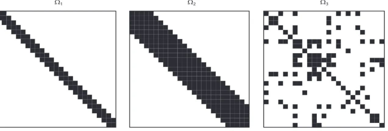
2.1 The zero patterns of the precision matrices specified in the models 1 (left), 2 (middle), and 3 (right) in the simulation study. Zero entries in the precision matrices are indicated in white color, while nonzero entries are in black. . . 15 2.2 Plots of true positive rates versus false positive rates as the threshold on

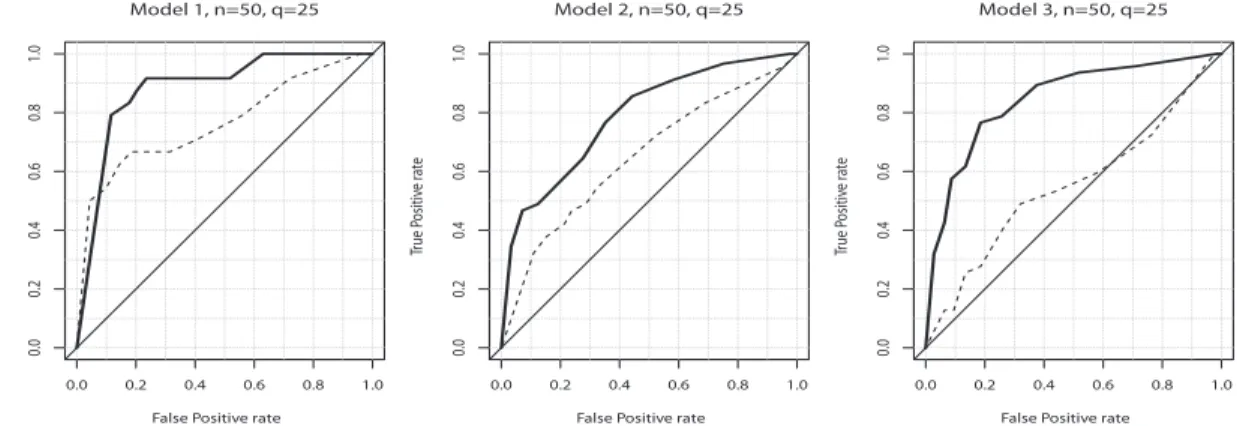
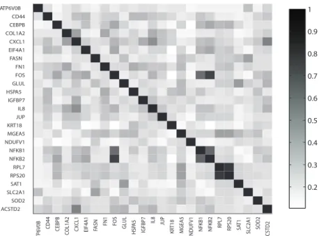
the posterior probabilities of inclusion in the model is varied (i.e. ROC curves). The curves are based on one simulation run under each of the three scenarios described in Section 2.4 and of the sample size n = 50 . The solid lines correspond to the ROC curves for the discrete graph models, while the dashed lines for the Gaussian graph models. . . 17 2.3 The color map displaying the GO-derived prior probabilities on edges.

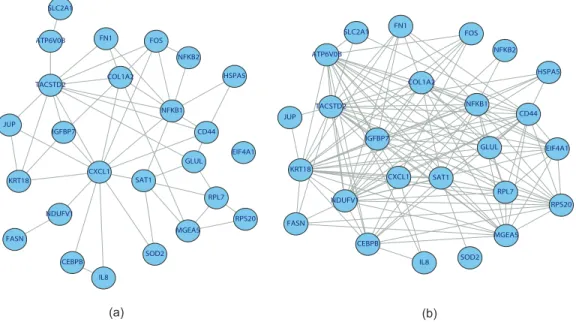
The probabilities are indicated by the color of the rectangles: the darker the color, the closer is the prior probability to 1 for the corresponding edge. 19 2.4 The inferred networks in real SAGE data analysis using the discrete

graphical model. (a) The prior for the graph G is derived from GO-based functional semantic similarities. (b) The prior forGis constant for all graphs. . . 20 3.1 Copy number profile from a tumor sample. The log-ratios are plotted on

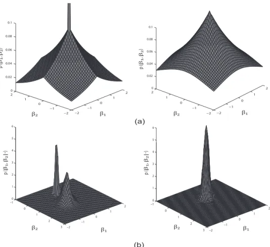
the vertical axis against their genomic position (in MB). The line type patterns indicate the gene structures on the chromosome. . . 26 3.2 Schematic plot of prior and posterior distribution of the hierarchical

struc-tured variable selection (HSVS) method. (a) Left: the density curve of an HSVS prior for a group with two variables; Right: a Bayesian lasso prior for a group with two variables. (b) Left: an example plot of the posterior distribution for a group with two variables when an HSVS prior is applied; Right: an example plot of the posterior distribution for the group of two variables when a Bayesian lasso prior is applied. . . 33

(9)

FIGURE Page 3.3 Data analysis results: (a) The posterior probabilities of being included in

the model in MCMC samples for the genes on chromosome 7 (left panel) and 12 (right panel). The dashed line indicates the FDR threshold where genes with probabilities above the line are considered significant; (b) The posterior median estimates with 95% credible intervals for the probes in two significant genes groups. The gene names are shown on the top of each plot. . . 48 3.4 Functional analysis of selected genes by the Ingenuity System. (a)

On-tology terms associated with the genes that have a gain or loss of copy numbers in the TNBC data; (b) Ingenuity pathway depicting oxidative phosphorylation. The complexes denoted by the solid ellipses show the points at which each of the five genes (enriched in copy-number) plays a role in this pathway. . . 49 3.5 Analysis results for the fused-HSVS model. (a) Comparison of the

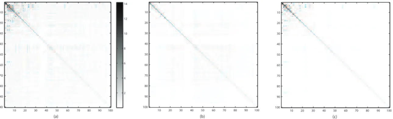
func-tional terms associated with the genes indicated by the HSVS (black color) and fused-HSVS (light grey color) methods. The plot is generated by the Ingenuity System; (b) Comparison of the coefficient estimates of a trun-cated MIP dataset for the HSVS model and fused-HSVS model. The left plot shows the posterior median estimates of the HSVS model with 95% credible intervals; the right plot shows the posterior median estimates of the fused-HSVS model with 95% credible intervals. The cross symbols in (b) are the coefficient estimates of the frequentist group lasso method.. . 53 4.1 Heatmaps of the absolute of covariance estimates by (a) sample covariance

(b) Bayesian decomposition method (c) LOREC estimator. . . 66 4.2 Scatter plots of the single factor loading identified by LOREC versus the

two factors loadings identified by the Bayesian decomposition model. The correlation between the two loading vectors on the left subplot is 0.98, and the correlation between the two loading vectors on the right subplot in 0.12. . . 67 4.3 Matrix plot indicating the sparse support of the residual covariance

com-ponent by (a) Bayesian decomposition method (b) LOREC estimator. . . 68 4.4 Graphical structure of model 6 in the simulations in Section 4.5.5 . . . . 77

(10)

4.5 Adjacency matrix of the genes involved in ER pathway depicting the graphical model of the residuals inferred by (a) Bayesian graphical fac-tor model for decomposable graph (b) Bayesian graphical facfac-tor model for unrestricted graph. Some genes have multiple sets of oligonuleotide sequences on the microarray, and hence the appearance of multiples of some genes: estrogen receptor itself (ESR1a, ESR1b), MYBL1 (MYBL1a, MYBL1b, MYBL1c, MYBL1d), TFF3 (TFF3a, TFF3b, TFF3c, TFF3d), XBP (XBP1a, XBP1b), and IGF1R (IGF1Ra, IGF1Rb). . . 79

(11)

1. INTRODUCTION

1.1 Problem Formulation

Significant advances in DNA sequencing strategies over the past decade have rev-olutionized the field of genomic research, allowing for development of many genome-wide technologies like microarray, serial analysis of gene expression (SAGE), RNA se-quencing, and molecular inverse probes (MIPs) experiments. These high-throughput technologies make deep genome sequencing and transcription quantification, and pro-vide information on up to thousands of genes simultaneously. Availability of vast amounts of high-dimensional data opens up a new opportunity to understand the mechanism of biological processes, and, as well, brings up challenges in methodol-ogy development for analyzing data of different types and characteristics. In this dissertation, we concern several important issues in genetic data analysis including graphical network modeling, feature selection, and covariance estimation. We pro-pose novel statistical methods and models to address the nature of different types of genetic data, and attempt to move towards more structured approaches to leverage information in statistical analysis.

1.2 Organization

In Section 2, we propose an algorithm for modeling gene networks based on dis-crete gene expression data. We specifically focus on the disdis-crete expression data from serial analysis of gene expression experiments (Velculescu et al., 1995). We assume that the observed counts of mRNA transcripts are from independent Poisson processes, with the mean rates to be the true transcriptional levels. The log ra-tios of the mean counts are considered to follow a multivariate normal distribution, whose inverse covariance matrix gives the conditional independence structure of the gene network model. We utilize a conjugate prior for the covariance matrices, the

(12)

hyper-inverse Wishart distribution introduced by Dawid and Lauritzen (1993), and an MCMC-based algorithm to identify graphical models. Furthermore, we propose a prior for the graphical models based on GO information, which utilizes prior in-formation on the genes of interest obtained in biological research as well as inducing sparsity in the graphical models as is assumed in gene regulatory networks. We con-duct simulation studies to examine the performance of our discrete graphical model and apply the method to real discrete datasets in identifying the gene regulatory networks.

In Section 3, we concern the issue of hierarchical feature selection in analysis of copy number data. Changes in chromosomal copy numbers have been identified as important causes of cancer (Pinkel and Albertson, 2005), and hence analysis of chromosomal copy number alterations has the potential to identify genetic markers and treatment targets for cancers. In this section, we consider a high-dimensional copy number profile obtained from molecular inversion probes experiments which measure probe copy number changes. Our goal is to ascertain probe-specific copy number alterations that are correlated with patient clinical characteristics. Since the probes located in the coding region of one gene can be taken as a natural group, we propose a Bayesian variable selection method, the hierarchical structured variable selection (HSVS) method, which accounts for the natural grouping structures in the data and simultaneously selects both gene groups and within-gene probes. The HSVS model utilizes a discrete mixture prior distribution for group selection and group-specific Bayesian lasso hierarchies for variable selection within groups. We further accounts for serial correlations within a gene by incorporating Bayesian fused lasso methods for within-group selection. Through simulations we establish that our method results in lower model errors than other methods when a natural grouping structure exists. We apply our method to an MIP study of breast cancer and show that it identifies genes and probes that are significantly associated with clinically relevant subtypes of breast cancer.

(13)

In Section 4, we consider the problem of estimating high-dimensional covariance matrices of a particular structure, which is a summation of low rank and sparse matrices. This covariance structure can be applied to multiple statistical models such as factor analytical model, random effects model, and conditional covariance model. We propose a novel Bayesian method of estimating the covariance matrices with such decomposition structure by rewriting the covariance model in the form of a factor analytic model where the number of latent factors is unknown. Our object is to estimate the covariance as well as recovering the rank of the low rank compo-nent and the support of the sparse compocompo-nent. We estimate the rank of the low rank component through factor selection with latent binary indicators, and use a Bayesian graphical lasso selection prior for the sparse component estimation. Simu-lation studies show that our method can recover the rank and the sparsity of the two components respectively with high frequencies. We further extend our method to a graphical factor analytic model, by which we recover the number of factors as well as the graphical model of the residuals. To induce sparsity in the inverse covariance of the residuals, we employ a hyper-inverse Wishart prior method for modeling decom-posable graphs, and a Bayesian graphical lasso method for unrestricted graphs. We show through simulations that the extended model can recover both the number of latent factors and the graphical model of the residuals successfully when the sample size is sufficient relative to the dimension.

Finally, we summarize our main findings and suggest future research directions in Section 5.

(14)

2. GRAPHICAL MODEL INFERENCE FOR DISCRETE GENE EXPRESSION DATA

2.1 Introduction

A gene network is a collection of genes that influence the expression levels of each other indirectly through their RNA or protein products. Gene network infer-ence is a task critical for revealing signaling pathways in cells, understanding the occurrence and development of diseases like cancers, and identifying target genes for disease treatment. With the development of genome-wide technologies like RNA fingerprinting, expressed sequence tag sequencing, serial analysis of gene expression (SAGE), and microarrays, high dimensional gene expression data become available for mapping the interactions between thousands of genes simultaneously. Current statistical modeling of gene networks is primarily based on continuous gene expres-sion profiles obtained from microarray experiments, with the gene expresexpres-sion data assumed to follow a Gaussian distribution, which has many well-established proper-ties.

In this section, we propose an algorithm for modeling gene networks based on discrete gene expression data. We specifically focus on the discrete data from SAGE experiments (Velculescu et al., 1995). In a SAGE experiment, all the mRNA tran-scripts of a cell sample are collected and a 10-base DNA fragment is released from each mRNA transcript, which is called a SAGE tag. The number of the tags with the same nucleotide sequence is then counted in a cell sample. Since the nucleotide sequence of a tag is specific to the mRNA from which the tag is released, the count of the tags of a particular sequence gives the amount of their corresponding mRNA transcripts in a cell sample. Note that the counts of mRNAs from SAGE experiments are relative quantities with respect to the total number of transcripts collected in a cell sample. In a typical SAGE experiment, a large number of mRNA transcripts (often from 30,000 to 100,000) are collected from each cell sample.

(15)

Similar to microarray, SAGE produces a snapshot of gene expression profiles by measuring the levels of mRNA transcription in a cell sample. However, SAGE pro-vides gene expression profiles with a higher level of genome coverage than microarray, because SAGE is not limited to expression analysis of known genes, as is microarray. Furthermore, SAGE experiments give the relative amount of each gene’s mRNAs with respect to the total mRNA transcripts in a cell sample. Thus we can compare mRNA levels among libraries generated by different laboratories. Due to these u-nique features of SAGE experiments, analysis of SAGE data plays an important role in biological and biomedical areas, such as prediction of new gene function and iden-tification of target genes for disease treatment. In this section, we explore discrete SAGE datasets for gene network structures with an undirected graph.

There have been many approaches to network modeling with Gaussian graphical models. In a Bayesian setting, Gaussian graphical models are based on hierarchical specifications for the covariance matrix (or precision matrix) using global conjugate priors on the space of positive-definite matrices, such as the inverse Wishart prior or its equivalents. Dawid and Lauritzen (1993) introduced an equivalent form as the hyper-inverse Wishart (HIW) distribution. This construction enjoys many advan-tages, such as computational efficiency, due to its conjugate formulation and exact calculation of marginal likelihoods (Scott and Carvalho, 2008). Giudici (1996) used a prior for the covariance matrix that is a mixture of HIW priors with fixed parameter-s over decompoparameter-sable graphparameter-s and calculated the poparameter-sterior probability of each graph. Armstrong et al. (2009) extended this method by proposing a prior that assigns equal probabilities over graph sizes and utilized a conditional Markov chain Monte Carlo (MCMC) sampler. These methods have been extended for nondecomposable graphs using reversible-jump algorithms (Giudici and Green, 1999; Brooks, Giudici, and Roberts, 2003). Moreover, the G-Wishart prior distribution has been proposed as a generalization of HIW priors that is suitable for nondecomposable graphs (Roverato, 2002; Atay-Kayis and Massam, 2005). Gaussian graphical models have been widely

(16)

used to infer the regulatory relationship among genes for continuous gene expression data at the transcriptional level (Wu, Ye, and Subramanian, 2003; Dobra et al., 2004; among others). The conditional independence arising out of a Gaussian graphical model is flagged by the zero off-diagonal elements in the inverse covariance matrix.

In this section, we develop Bayesian graphical models for discrete gene expres-sion data. We assume that the observed counts of mRNA transcripts in a SAGE experiment are from Poisson processes, with the means to be the true transcriptional levels. The log ratios of the mean counts are considered to follow a multivariate nor-mal distribution. That is, the expression levels of genes are regulated by each other through a Gaussian graphical model underlying the log ratios of the means, whose inverse covariance matrix gives the conditional independence structure of the undi-rected gene network. We utilize the conjugate HIW prior to sample the covariance matrices and an MCMC-based algorithm to identify graphical models. Furthermore, we propose a prior for the graphical models based on GO information, which utilizes prior information on the genes of interest obtained in biological research as well as inducing sparsity in the graphical models as is assumed in gene regulatory networks. We obtain the GO information from the GO consortium, which provides a con-trolled vocabulary of terms describing gene product characteristics in the aspects of cellular component, molecular function, and biological process (Ashburner et al., 2000). For each of the three fields, GO terms are organized in a hierarchical di-rected acyclic graph (DAG) structure, reflecting the associations between ontology terms. For example, the biological process terms “calcium-mediated signaling” and “leukemia signaling” are two daughter terms of the term “intracellular signaling,” meaning that they are two kinds of intracellular signaling; and “intracellular signal-ing” is a daughter term of “signaling transduction.” Hence, two genes sharing the same or similar GO terms in biological process may have the same or similar cellular functions. Based on this idea, methods have been developed to measure the semantic similarity between GO terms and gene products (Resnik, 1999; Wang et al., 2007).

(17)

These gene similarity measures based on associated GO terms have been used in gene clustering and gene function prediction (Kustra and Zagdanski, 2006).

In our method, we apply GO-derived semantic similarity measurements to gene network modeling. We measure the functional semantic similarity of each pair of the genes of interest based on the relatedness of their associated GO terms. The semantic similarity score is then taken as the prior probability of an edge between the two genes in the gene network. Using this method, we derive a prior for the graphical model by taking the product of the prior probabilities of the edges in the graph. This GO-based prior on the gene network incorporates biological information of the genes into gene network modeling as well as bringing scientifically interpretable sparsity in the inferred graphical models.

We introduce our Bayesian hierarchical model and the GO-based prior derivation in Section 2.2. We describe a model selection method based on false discovery rates (FDRs) for inferring graphical models from posterior samples in Section 2.3. In Section 2.4, we show the results of a simulation study evaluating the performance of the discrete graph modeling method. In Section 2.5, we present the result of a real SAGE data analysis to model the gene networks in breast cancer cells. Finally, a short summary of our method is included in Section 2.6. The schemes of posterior sampling are detailed in Appendix A.

2.2 Probability Model

LetX denote ann×q matrix of discrete gene expression profiles, with Xij to be

the observed mRNA count of gene j (j = 1,· · · , q) obtained in a SAGE experiment for theith_(i_{= 1,}_{· · ·} _{, n) individual. Since a SAGE experiment counts the transcripts} of a gene given a large total number of transcripts in a cell sample, we assume that each count, Xij, follows a Poisson distribution with mean λij. We consider λij, the

expected count of the transcripts given a total number of transcripts, as the true transcriptional expression amount of gene j in the ith _{cell sample. We assume that}

(18)

the log ratios of λi = (λi1, ..., λiq)0 for i = 1,· · · , n follow a multivariate normal

distribution Np(µ,Σ). The likelihood is specified as follows:

Xij ∼ P ois(λij),

log(λi) ∼ Nq(µ,Σ).

This is a special case of popular generalized linear mixed models (Zeger and Karim, 1991; Breslow and Clayton, 1993). In this framework, we assume a graphical model through Σ to account for the association structure among the underlying log ratios of the expression levels in a cell sample. Our focus is to infer the graphical model by selecting the covariance matrix Σ.

2.2.1 Bayesian Gaussian Graphical Models

In a Bayesian framework, Gaussian graphical modeling is based on hierarchical prior specifications for the covariance matrix Σ at the two levels: a prior distribution for Σ under each graph and a prior distribution over different graphs. Before giving the details about the hierarchical priors, we first describe the notations on Gaussian graphical models.

An undirected graph is a pair of G = (V, E) with a vertex set V = {1, ..., q} and an edge set E ⊆ V ×V. Nodes i and j are adjacent or connected in G if (i, j) ∈ E, whereas i and j are conditionally independent if (i, j) ∈/ E. A graph G with E =V ×V is called a complete graph. Complete subgraphs C ⊂V are called cliques; the joint subset of two cliques is called a separator S. If a graph G could be partitioned into a sequence of subgraphs (C1, S2, C2, ..., CK) such thatV =S_kCk

and Sk = Ck−1TCk are complete for all k = 1, ..., K, G is called a decomposable

graph (Lauritzen, 1996). In this section, we consider the decomposable graphs. For a covariance matrix Σ, let Ω = Σ−1be the inverse covariance matrix, or the precision matrix. Nodes iand j are conditionally independent, given other nodes, if and only

(19)

if Ωij = 0. Thus, the undirected graph G is given by the configuration of nonzero

off-diagonal elements of Σ: E ={(i, j) : Ωij 6= 0}.

LetM(G) be the set of all symmetric positive-definite matrices Σ satisfyingE = {(i, j) : Ωij 6= 0}. Given a decomposable graph G = (V, E), Dawid and Lauritzen

(1993) introduced the HIW distribution for a covariance matrix Σ ∈ M(G), with parameters (δ,Φ), denoted by Σ ∼ HIW(G, δ,Φ). The probability density function (pdf) is given by p(Σ|G, δ,Φ) = QK k=1p(ΣCk|δ,ΦCk) QK k=2p(ΣSk|δ,ΦSk) ,

where δ∈R+ is a degree-of-freedom parameter, Φ ∈M(G) is a symmetric positive-definite scale matrix, and Ck and Sk are the cliques and separators of the graph G

respectively. The terms p(ΣCk|δ,ΦCk) denote the inverse Wishart (IW) density of

ΣCk ∼IW(δ,ΦCk) with the pdf

p(ΣCk|δ,ΦCk)∝ |ΣCk| −(δ/2+|Ck|)_exp −1 2tr(Σ −1 CkΦCk) .

The HIW distribution is a conjugate prior distribution for the covariance matrix Σ∈M(G). Specifically, if q-dimensional random variablesXi follow an independent

and identical (iid) multivariate normal distribution Nq(0,Σ) for i = 1, . . . , n, and

Σ follows HIW(G, δ,Φ), the posterior of Σ is Σ|X, G ∼ HIW(G, δ+n,Φ +X0X). The closed form of the posterior distribution for Σ plays a key part in the posterior inference based on an MCMC algorithm.

(20)

2.2.2 Hierarchical Model

To facilitate computation and notation, we reparameterize log(λij) asθij

through-out the rest of the section. We assume the complete hierarchical model for a discrete gene expression dataset as follows:

Xij ∼ P ois(λij), (2.1) θi ∼ Nq(µ,Σ)., (2.2) p(µ|Σ, G) ∝ constant, (2.3) Σ|δ, r, G ∼ HIW(G, δ, rIq), (2.4) r ∼ Unif(0, c), (2.5) G ∼ π(G), (2.6)

where δ, r, and c are fixed, positive hyperparameters and Iq is a q × q identity

matrix. Equations (2.3) and (2.4) specify the prior for the mean and covariance matrix, respectively. We assume an improper constant prior forµ, as our focus is on the structures of Σ−1. The prior for Σ is HIW(G, δ,Φ) as described in Section 2.2.1. We restrict the graphGof Σ to be decomposable so that the prior for Σ is a mixture of HIW distributions over all decomposable graphs. We consider δ= 3 as reflecting the lack of prior information on Σ, and specify the hyperparameter Φ as rIq, where

r is assumed to follow a uniform hyperprior on the interval (0, c) as in equation (2.5) for some large value of c.

Notice that given the priors forµ and Σ as specified above, we can integrate out

µ and Σ and obtain a marginalized prior on θ given the graph G as p(θ|G, δ, r)∝ h(G, δ, rIq)

h(G, δ+n−1, rIq+Sθ)

(21)

whereSθ =Pn_i₌₁(θi−θ¯)(θi−θ¯)0. The term h(G, δ, rIq) is the normalizing constant

for the HIW(G, δ, rIq) distribution given by

h(G, δ, rIq) = QK k=1| rI_Ck 2 | (δ+|Ck₂|−1)_Γ| Ck| δ+|Ck|−1 2 −1 QK k=2| rI_Sk 2 | (δ+|Sk₂|−1)_Γ |Sk| δ+|Sk|−1 2 −1, where Γq(x) = πq(q−1)/4 Qq

j=1Γ(x+ (1−j)/2) is the multivariate gamma function. The marginalized prior leads to a collapsed Gibbs algorithm in sampling G, which substantially accelerates the graphical model search task and is valued when the graph G is our focus in the inference.

We induce the prior π(G) in equation (2.6) by assigning an independent pri-or probability of an edge, p(eij), to each pair of nodes (i, j), so that π(G) =

Q

(i,j)∈Ep(eij = 1)·

Q

(i,j)∈/Ep(eij = 0). Without prior information, a choice of p(eij)

could be the Bernoulli-Beta hierarchical prior. Scott and Berger (2010) showed that when the hyperparameters of the Beta distribution is (1,1), the marginalized prior probability of a graphical model containing k edges out ofq(q−1)/2 potential edges in a graph G is p(k)∝ q(q−1)_k /2−1

. Hence, such choice of prior encourages sparsity in the inferred graphical models. In the context of gene expression network model-ing as in the section, we borrow information on relatedness between genes based on biological studies and derive a prior π(G) from the ontology terms associated with the genes of interest.

2.2.3 GO-based Prior for G

As mentioned above, GO terms describe gene product characteristics in a con-trolled vocabulary. A pair of genes with the same or closely related ontology terms in biological process are thought to be potentially associated in signaling pathway or expression regulation. We measure the relatedness of all pairs of genes in terms of their associated ontology terms and derive the priors p(eij) that are proportional

(22)

to the measurements. Here we use the functional semantic similarity as a measure of the relatedness of two genes.

The semantic similarity measures the similarity of two GO terms by evaluating how much information the two terms share. Here we use Wang et al.’s measure (Wang et al., 2007), which is based on the relative locations of the terms in the DAG structure of the GO graph and their semantic relations with the ascendant terms that subsume the two terms. For a GO term A, let TA denote the set of all its

ancestor terms including term Aitself, and SA(t) be defined as the contribution of a

term t ∈ TA to the semantics of A based on the relative locations of t and A in the

GO graph. The semantic similarity score between two GO terms (A,B) is defined as follows: SGO(A, B) = P t∈TA∩TB SA(t) +SB(t) P t∈TASA(t) + P t∈TBSB(t) ,

which is within (0,1). Usually one gene is annotated by many GO terms. The functional similarity between two genes G1 and G2, Sim(G1, G2), is then calculated by averaging the semantic similarity scores for all pairs of their associated terms. The functional similarity score between any two genes (Gi, Gj) is within (0,1), where a

value close to 0 indicates the two genes unlikely to be related and a value near 1 indicates close relatedness of the two genes in cellular functioning. Hence, we consider the score as a natural prior probability of an edge between the two genes, i.e. p(eij = 1) =Sim(Gi, Gj).

We derive the prior for the graphG = (V, E) based on the GO similarity scores as: π(G) = Y (i,j)∈E p(eij = 1) Y (i,j)∈/E p(eij = 0), = Y (i,j)∈E Sim(Gi, Gj) Y (i,j)∈/E {1−Sim(Gj, Gj)}.

(23)

With the above prior on the graph G, we actually assign a prior probability to the existence or absence of each edge in the graph. As a high similarity score between two genes reflects their potential relatedness in gene regulation, the specified prior favors the graph model that includes edges between semantically similar genes.

2.3 Model Selection Using False Discovery Rates

The posterior sampling schemes we have outlined explore the model space and result in MCMC samples of graph Gat each iteration. One method of summarizing the information in the samples is to pick the graph model that is visited mostly by the sampler. However, this particular graph may only appear in a very small proportion of MCMC samples. An alternative strategy is to utilize all of the MCMC samples and average over the various models visited by the sampler. This model averaging approach weighs the evidence of significance for each edge separately using all MCMC samples. We outline an approach to conduct Bayesian model selection based on controlling the false discovery rate (FDR) (Benjamini and Hochberg, 1995). Suppose we have T posterior samples of graph G = (V, E) from an MCMC computation, which are represented as T sets of edge indicators {e(_ijt) : i < j}. If (i, j)∈E(t) _{we have} _e(t)

ij = 1; else e

(t)

ij = 0. Letpij represent the posterior probability

of including the edge (i, j) in the graph. We can estimate pij to be the relative

number of times the edge (i, j) is present in the graph across theT MCMC samples:

pij = 1 T T X t=1 I{e(_ijt) = 1},

where I(·) is an indicator function.

We assume that for some significance threshold φ, any edge (i, j) with pij > φ

is considered as significant and is included in the graph G. Then the graph with E = {(i, j) :pij > φ} includes all the edges considered to be significant. Note that

(24)

measure the probability of a false positive if an edge (i, j) is significant but not in the true graph. The significance threshold φ can be determined based on classical Bayesian utility considerations, such as in M¨uller et al. (2004), based on the elicited relative costs of false positive and false negative errors, or can be set to control the overall average Bayesian FDR. (See Morris et al., 2008; Baladandayuthapani et al., 2010; and Bonato et al., 2011 for detailed expositions in other settings).

Thus given a global FDR bound α ∈ (0,1), we are interested in finding the threshold value φα for flagging the set of edges {(i, j) : pij > φ} as potentially

relevant and labeling them as discoveries. This implies that the threshold φα is a

cut-off on the (model-based) posterior probabilities that corresponds to an expected Bayesian FDR ofα, which means that 100α% of the edges identified as discoveries are expected to be false positives. The threshold φα is determined in the following way:

For all (i, j) :i < j, we sort pij in descending order to yieldp(k), k = 1, ..., q(q−1)/2.

Then, φα = p(ξ), where ξ = max{(k∗) :

Pk∗

k=1(1−p(k))/k∗ ≤ α}. The set of edges {(i, j) : pij > φα} can be claimed to be positive in the graph based on an average

Bayesian FDR of α.

2.4 Simulation Study

In this section, we conduct a simulation study to examine the performance of our method. We setq= 25 and consider three scenarios that portray different complexity levels of the networks in generating data. We assume that the discrete data matrix X is generated from the model,

Xij ∼ P ois(eθij), θi ∼ Nq(µ,Σ),

where θi = (θi1, . . . , θiq)0. The covariance matrix, Σ, or its corresponding precision

(25)

• Model 1: We assume that Σ is the covariance matrix of a Gaussian AR(1) process with the element σij = 0.7|i−j|. The specification of Σ corresponds

to a band-diagonal precision matrix Ω of bandwidth 1, where only 4% of the off-diagonal elements are zero.

• Model 2: We assume that Σ is the covariance matrix of a Gaussian AR(4) process with the element of Ω = Σ−1 to be ωij = 2I{|i−j|= 0} −0.5I{|i−j|= 1} −0.8I{|i−j|= 2}+ 0.2I{|i−j|= 3}+ 0.3I{|i−j|= 4}. The precision matrix Ω is a band-diagonal matrix of bandwidth 4, where 30% of the off-diagonal elements are zero.

• Model 3: The true decomposable graph G is specified such that about 15% of the off-diagonal elements in the corresponding precision matrix are set to be zero. The true Σ is then generated from the HIW distribution HIW(G,3,Φ) conditional on the graph G, where Φ is an arbitrary positive definite matrix. The configurations of the nonzero off-diagonal elements in the precision matrices as specified in models 1, 2, and 3 are shown in Figure 2.1. For each model, datasets

Ω1 Ω2 Ω3

Fig. 2.1. The zero patterns of the precision matrices specified in the models 1 (left), 2 (middle), and 3 (right) in the simulation study. Zero entries in the precision matrices are indicated in white color, while nonzero entries are in black.

(26)

are generated of three sample sizesn= 25,50,and 100. Our proposed Bayesian model for discrete data is used to estimate the network structure based on the posterior samples of 15,000 iterations after 5,000 burn-in iterations. The prior for the graph π(G) is taken to be constant since no biological GO information is available for simulated data.

For comparison, we transform the simulated data into log ratios, and assume a Gaussian graphical model for the log-transformed data with the hierarchy:

log(Xi) ∼ Nq(µ,Σ).,

p(µ|Σ, G) ∝ constant, Σ|δ, r, G ∼ HIW(G, δ, rIq),

r ∼ Unif(0, c), G ∼ π(G).

The above Gaussian graphical model has the same hierarchical priors on µ and Σ as in our discrete graphical model, but has a different likelihood. The posterior distributions and the MCMC sampling schemes of the parameters µ,Σ, r, G are the same as described in Appendix A except that the log(θ) is replaced with log(X).

To evaluate the performance of the methods, we calculate the true positive rates (TPRs) and the false positive rates (FPRs) defined as

T P R= T P

T P +F N, F P R=

F P T N +F P,

where TP, FP, TN, and FN denote the number of true positive, false positive, true negative, and false negative edges, respectively. Figure 2.2 shows the plots of TPRs versus FPRs as we vary the decision threshold on the posterior probabilities of edge inclusion, which are called the receiver operating characteristic (ROC) curves, based on one simulation result under each of the three settings and n = 50. The figure

(27)

shows that the ROC curves of the discrete graph models are closer to the upper left corner than those of the Gaussian graph models for the three simulation settings, indicating a better performance of our method in estimating the discrete graphs.

Table 2.1 summarizes the mean numbers of false positive edges and false negative edges over 20 replications. The graph models are selected as described in Section 2.3 based on thresholds corresponding to an FDR of α = 0.20. In accordance with the ROC curves, the discrete graph models have significantly fewer false negatives than the Gaussian graph models, suggesting a higher sensitivity of our method to the edges in a graph. As the sample size increases, both the FPRs and the FNRs decrease obviously in our discrete graph models compared with those in the Gaussian graphical models. When the sample size increases to 100, our method estimates the discrete models optimally, especially for the sparse model, model 1, which has FPRs of less than 10% on average and FNRs of 0%.

0.0 0.2 0.4 0.6 0.8 1.0 0. 00 .2 0. 40 .6 0. 81 .0 Model 1, n=50, q=25

False Positive rate

Tr ue P ositi ve rate 0.0 0.2 0.4 0.6 0.8 1.0 0. 00 .2 0. 40 .6 0. 81 .0 Model 2, n=50, q=25

False Positive rate

Tr ue P ositi ve rate 0.0 0.2 0.4 0.6 0.8 1.0 0. 00 .2 0. 40 .6 0. 81 .0 Model 3, n=50, q=25

False Positive rate

Tr ue P ositi ve rate

Fig. 2.2. Plots of true positive rates versus false positive rates as the threshold on the posterior probabilities of inclusion in the model is varied (i.e. ROC curves). The curves are based on one simulation run under each of the three scenarios described in Section 2.4 and of the sample size n = 50 . The solid lines correspond to the ROC curves for the discrete graph models, while the dashed lines for the Gaussian graph models.

(28)

2.5 Real Analysis

2.5.1 SAGE Dataset and Pre-Processing

We apply our algorithm in modeling the gene expression network of 25 genes. These genes are identified to be differentially expressed in breast cancer cells by com-parison of SAGE expression files followed by statistical tests (Allinen et al., 2004; Porter et al., 2001). The SAGE dataset of these 25 genes is composed of 50 SAGE li-braries obtained from carcinoma breast tissue cells. These lili-braries are publicly

avail-able for sharing at the Human SAGE Genie website

(http://cgap.nci.nih.gov/SAGE). This website, motivated by the Cancer Genome Anatomy Project (CGAP), is a platform where researchers share their SAGE dataset-s that are generated from diverdataset-se cancer and normal tidataset-sdataset-suedataset-s in many laboratoriedataset-s. Sequencing resources vary across laboratories, so each SAGE library has a different total number of tags. As a consequence, the variances of errors are not in the same

Table 2.1

Simulation results under different network reconstruction methods for model 1, 2, and 3. The mean false positive edges and the mean false negative edges over 20 replications are presented in the table with the standard deviations in parentheses. FP: false positive; FN: false negative. See Section 2.4 for details about the models.

true graph discrete graph model Gaussian graph model Model n No edges Edges FP edges FN edges FP edges FN edges Model 1 25 276 24 71.45 (14.84) 5.45 (1.43) 65.15 (12.98) 9.65 (1.98) 50 276 24 49.55 (13.33) 0.65 (0.81) 60.70 (10.75) 6.55 (1.79) 100 276 24 23.95 ( 5.06) 0.00 (0.00) 50.65 ( 8.91) 3.10 (1.55) Model 2 25 210 90 64.00 (10.02) 45.10 (4.74) 54.30 ( 9.92) 52.95 (5.40) 50 210 90 48.65 (14.41) 30.35 (4.43) 55.35 ( 8.66) 46.75 (4.51) 100 210 90 26.60 ( 8.21) 11.40 (3.36) 52.05 (12.69) 37.55 (4.13) Model 3 25 253 47 50.85 (10.58) 19.95 (2.80) 52.50 (11.47) 30.80 (4.11) 50 253 47 43.60 (10.56) 14.70 (2.25) 48.30 (10.17) 26.60 (3.94) 100 253 47 26.80 ( 8.47) 9.80 (2.86) 39.70 ( 8.35) 19.05 (3.91)

(29)

scale. Hence, we normalize the tag frequencies in each library by scaling them so that the total numbers of tags are 20,000 in all libraries.

2.5.2 The Inferred Gene Expression Network

The functional semantic similarity is calculated for each pair of the 25 genes of interest as discussed in Section 2.2.3 using the Bioconductor package GOSemSim

(Yu et al., 2010). The semantic similarity scores are obtained for biological process GO terms for each pair of genes. Figure 2.3 shows the intensities of the calculated priors on the edges between all pairs of genes in a color map, where the darkness of a lattice is proportional to the prior probability of including the edge in a graph. The prior on a graph is then assigned as the product of the prior probabilities as discussed in Section 2.2.3. ACSTD2 SOD2 SLC2A1 SAT1 RPS20 RPL7 NFKB2 NFKB1 NDUFV1 MGEA5 KRT18 JUP IL8 IGFBP7 HSPA5 GLUL FOS FN1 FASN EIF4A1 CXCL1 COL1A2 CEBPB CD44 ATP6V0B A TP 6 V0B CD 4 4 CE B PB CO L 1A 2 CX CL 1 EI F4 A1 F AS N FN1 FOS GL U L HSP A5 IG FB P7 IL8 _JUP KR T18 MG E A5 ND U FV 1 NF K B1 NF K B2 RPL7 RPS20 SA T1 SLC 2A 1 SO D 2 TA CS T D2 0.2 0.3 0.4 0.5 0.6 0.7 0.8 0.9 1

Fig. 2.3. The color map displaying the GO-derived prior probabil-ities on edges. The probabilprobabil-ities are indicated by the color of the rectangles: the darker the color, the closer is the prior probability to 1 for the corresponding edge.

(30)

The proposed Bayesian discrete graphical model is applied to the discrete SAGE data to estimate the network structure and model selection is based on the posterior samples of 50,000 iterations after 10,000 burn-in iterations. The Bayesian estimates of the graphs are obtained by averaging each edge separately and graph models are selected based on an FDR of α = 0.20. The resulting gene network is displayed in Figure 2.4 (a), which is partially supported by biological studies.

The genes NFKB1 and NFKB2 encode the subunits of a transcription factor NF-κB, which is known in biological research to stimulate the expression of genes involved in a wide variety of biological functions. The target genes of NF-κB include CD44, COL1A2, CXCL1, FOS, FN1, HSPA5, SAT1, and TACSTD2, which are identified in our inferred network. The promoters of these target genes are all found to contain the NF-κB binding site for transcriptional regulation. Biological studies also find that TACSTD2, the gene encoding a cell surface receptor, transduces an

(a) (b) ATP6V0B CD44 CEBPB COL1A2 CXCL1 EIF4A1 FASN FN1 _FOS GLUL HSPA5 IGFBP7 IL8 JUP KRT18 MGEA5 NDUFV1 NFKB1 NFKB2 RPL7 RPS20 SAT1 SLC2A1 SOD2 TACSTD2 ATP6V0B CD44 CEBPB COL1A2 CXCL1 EIF4A1 FASN FN1 FOS GLUL HSPA5 IGFBP7 IL8 JUP KRT18 MGEA5 NDUFV1 NFKB1 NFKB2 RPL7 RPS20 SAT1 SLC2A1 SOD2 TACSTD2

Fig. 2.4. The inferred networks in real SAGE data analysis using the discrete graphical model. (a) The prior for the graphGis derived from GO-based functional semantic similarities. (b) The prior for G is constant for all graphs.

(31)

intracellular calcium signal and contributes to tumor pathogenesis by activating the ERK/MAPK pathway (Cubas et al., 2010). This discovery is consistent with the constructed gene network in which TACSTD2 is connected to FOS, NF-κB, and IGFBP7, which are involved in the ERK/MAPK pathway.

The gene COL1A2 encodes one of the chains for type I collagen, the major com-ponent of extracellular matrix in skin and other tissues. Research in biology has found that the synthesis of the chain is highly regulated by different cytokines and transcription factors at the transcriptional level. These protein factors involved in COL1A2 regulation include AP1, a family of transcription factors containing the protein product of FOS; NF-κB, the protein product of NFKB1/2; ERK1/2, which can be activated by TACSTD2; and IGFs, which interact with IGFBP7-encoded proteins (Ghosh, 2002). The protein product of FN1 gene is also known to interact with the chain of type I collagen encoded by COL1A2 (Sipes et al., 1993). These findings directly support the dependency between COL1A2 and its neighbors in the inferred gene network. Some other biological discoveries also agree with our network such as the transcriptional regulation of IL-8 by CEBPB (Weber et al., 2003) and SOD2-related oxidative stress induced expression of CXCL1 (Wu et al., 2009).

To test the sensitivity of the network inference to the GO-derived prior probabili-ties, we reanalyze the real data without the priors induced based on GO information, i.e. the prior of each graph is constant. The resulting network as shown in Figure 2.4 (b) is much more complex than the GO-based network, including more than 100 edges between the 25 genes.

2.6 Discussion

In this section, we extend the Bayesian graphical model for gene networks to dis-crete expression data from SAGE experiments. We model the count data of mRNA transcripts with independent Poisson distributions, and assume that the log ratios of the Poisson means follow a multivariate normal distribution, whose inverse

(32)

covari-ance matrix gives the conditional independence structure of the gene network. We utilize a conjugate prior for the covariance matrix and a collapsed Gibbs sampling algorithm for a fast graphical model search. In addition, we incorporate biological information on genes in our algorithm, by measuring the GO-based semantic similar-ity between each pair of genes as the prior for a graph. The derivation of GO-based priors is rooted in the biological characteristics of gene regulation. Regulation of gene expression usually occurs between two genes involved in the same metabolic or signaling pathways. Hence, two genes with unrelated gene functions are unlikely to have a direct regulation relationship.

Simulation studies show that our method of modeling discrete gene expression data estimates the network structures with lower FNRs and FPRs than the Gaus-sian graphical models that are applied to the log-transformed data. In addition, simulation results show that our discrete graph model performs obviously better as sample size increases, and leads to optimal predicted models for moderate sample-size/dimension ratios (=4). We also apply this algorithm to a real SAGE dataset of 25 genes. We show in the result that the derived gene network model with our method agrees with some discoveries in the traditional biological research, which partially supports our model.

(33)

3. BAYESIAN HIERARCHICAL STRUCTURED VARIABLE SELECTION METHODS WITH APPLICATION TO MIP STUDIES IN BREAST CANCER

3.1 Introduction

3.1.1 Molecular Inversion Probe-based Arrays for Copy Number Mea-surement

Changes in chromosomal copy numbers have been identified as important caus-es of cancer (Pinkel and Albertson, 2005). Chromosomal copy number alteration (CNA) can lead to over-expression of pro-oncogenes or silence of tumor suppressor genes, and affect cellular functions in cell division or programmed cell death (Guha et al., 2008). The accumulation of these DNA errors will eventually influence the devel-opment or progression of carcinogenesis; hence, chromosomal copy number analysis has the potential to elucidate tumor progression and identify genetic markers for cancer diagnosis and treatment. CNAs, as gains and losses, are frequent events in breast tumors and occur in patterns that are thought to distinguish genetic paths to tumorigenesis and influence the clinical behavior of the disease (Rennstam et al., 2003; van Beers and Nederlof, 2006).

Many techniques have been developed for the genome-wide detection of CNAs, such as array-based comparative genomic hybridization (CGH), bacterial artificial chromosome CGH, and oligonucleotide array-based CGH (Pinkel et al., 1998; Iafrate et al., 2004; Lucito et al., 2003). A technique that has recently been used for the measurement of allele copy numbers is the molecular inversion probe (MIP) (Hard-enbol et al., 2003; Wang et al., 2007). Unlike other CNA measuring techniques such as the CGH methods, the MIP assay requires sequences at the ends to bind genomic DNA simultaneously and utilizes enzymatic steps (ligation) to capture specific loci. The circularization method ensures a high degree of specificity in identifying the loci of interest and reduces cross-talk between probes. The MIP assay generates

(34)

genotype data as well as copy numbers, which can be used for sample tracking and data quality assessment. Most banked samples with clinical follow-up data are from formalin-fixed, paraffin-embedded (FFPE) tissues, which generally show degraded DNA in the cells. Wang et al. (2007) show that the MIP technology, which requires only a small (∼40bp) target binding site, is more accurate in measuring probe copy numbers for degraded FFPE-derived DNA. Other advantages of the MIP assay are the low amount of DNA sample required, its high levels of multiplexing, and its reproducibility. Refer to Hardenbol et al. (2003) and Wang et al. (2007) for more detailed descriptions of the MIP assay.

In this section, we focus on the analysis of a novel high-dimensional MIP dataset from 971 samples of early-stage breast cancer (stages I and II) collected through the Specialized Programs of Research Excellence (SPORE) in breast cancer at the University of Texas MD Anderson Cancer Center for the purpose of improving risk prediction for disease recurrence. The dataset includes full genome quantifications for 330,000 MIPs from tumor cells of patients using high-density OncoscanTMarrays from AffymetrixTM_{. A detailed description of the dataset with regard to data collection,} pre-processing and normalization is provided in Section 3.6.1. Briefly, the resulting (normalized) data for downstream statistical analysis consist of the log₂ intensity ratios of the copy numbers in test samples to the copy numbers in normal reference cells for all probes. Hence, for a cell sample with the normal probe copy number (= 2), the normalized value is log₂(2/2) = 0; for a probe with a gain of measured copy numbers (> 2) the log ratio is positive, and for a probe with a loss of copy numbers (< 2) the log ratio is negative. The magnitudes of intensity ratios in the positive and negative direction are indicative of multiple probe-level gains and losses, respectively.

In addition to the MIP copy number profiles, we have data on a number of relevant clinical outcomes from these patient samples, such as the clinical subtype of breast cancer defined by tumor markers (i.e., hormone receptor status, HER2 status, Ki67),

(35)

tumor size, and lymph node status, as well as other clinicopathological characteristics such as age, stage, tumor grade, histology, and type of treatment (Thompson et al., 2011). Our main focus in this section is to identify MIPs that are significantly associated with the clinical and pathologic characteristics of the tumors with an emphasis on clinical subtypes. Discovering and validating CNAs that correlate with tumor characteristics will identify regions of high interest for further investigation as clinically useful diagnostic and treatment biomarkers.

We assume that many of the acquired chromosomal events act jointly in medi-ating the biological effects. Thus it is of high interest to model the joint effects of CNAs detected using the MIP probes and discover regions of the genome that exhibit significant associations – in contrast to univariate single MIP analysis, which might miss regions with weak marginal but important joint effects on the clinical outcomes. However, inferential challenges for the MIP copy number dataset include not only its high-dimensionality but also that markers tend to be spatially correlated because the MIPs are indexed by genomic location. We propose a novel structured “hunt-ing” approach to identify areas of the genome that are significantly associated with clinically relevant outcomes. We follow the two-level hierarchical structure induced by biology: a gene level and MIP-within-gene level architecture. Thus we group contiguous MIPs (as per their genomic location) by their unique gene annotation and treat the genes (group) as the first level of the hierarchy and the MIPs within the genes (subgroup) as the second level of the hierarchy.

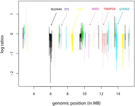
To illustrate our main idea, in Figure 3.1 we show an example plot of the partial MIP copy number profile for a randomly selected patient sample, where the x-axis is the genomic location and each vertical line is the log-intensity ratio for an MIP probe. The different line type patterns correspond to the gene groups, indicating the uniquely annotated gene structures on the chromosome. There are several features exemplified in the plot. There exists substantial variability both within and between the genes, primarily due to different numbers of probes mapped to each gene and

(36)

different probes within the same gene contributing differently, both positively and negatively. Also there exists serial correlation between the probes within the same gene, given their proximity by genomic location. Biologically, our gene-centric se-lection approach is of more interest to our scientific collaborators since there exists substantial knowledge about genes as functional units and the analytic result is more interpretable in terms of a medical diagnosis. In addition, for a specific gene, differ-ent probes may confer differdiffer-ent factors to the gene’s function and thus it is of equal interest to identify predictive probes within a selected gene. Therefore, in our study, we want to select both genes and within-gene probes that are significantly associated with clinically relevant outcomes – leading to a statistical formulation ofhierarchical structured variable selection.

4 6 8 10 12 14

−2

−1

0

1

genomic position (in MB)

log ratios

NLGN4X STS KAL1 MID1 FRMPD4 GPM6B

Fig. 3.1. Copy number profile from a tumor sample. The log-ratios are plotted on the vertical axis against their genomic position (in MB). The line type patterns indicate the gene structures on the chromosome.

(37)

3.1.2 Relevant Statistical Literature

Variable selection is a fundamental issue in statistical analysis and has been extensively studied. Penalized methods such as the bridge regression (Frank and Friedman, 1993), the lasso regression (Tibshirani, 1996), the SCAD regression (Fan and Li, 2001), the LARS regression (Efron et al., 2004) and the OSCAR regression (Bondell and Reich, 2008) have been proposed due to their relatively stable perfor-mance in model selection and prediction. The lasso method has especially gained much attention. It utilizes anL1-norm penalty function to achieve estimation shrink-age and variable selection. In a Bayesian framework, the variable selection problem can be viewed as the identification of nonzero regression parameters based on pos-terior distributions. Different priors have been considered for this purpose. Mitchell and Beauchamp (1988) propose a “spike and slab” method that assumes the prior distribution of each regression coefficient to be a mixture of a point mass at 0 and a diffuse uniform distribution elsewhere; this is extended by George and McCulloch (1993; 1997), Kuo and Mallick (1998), and Ishwaran and Rao (2005) in different settings. Other methods specify absolutely continuous priors that approximate the “spike and slab” shape, shrinking the estimates toward zero (Xu, 2003; Bae and Mallick, 2004; Park and Casella, 2008; Griffin and Brown, 2007; 2010). In particu-lar, Park and Casella (2008) extend the frequentist lasso with a full Bayesian method by assigning independent and identical Laplace priors to the regression parameters. The above mentioned methods ignore the grouping structure that appears in many applications such as ours. The individual-level variable selection methods tend to select more groups than necessary when selection at group level is desired. To accommodate group-level selection, Yuan and Lin (2006) propose the group lasso method, in which a lasso penalty function is applied to theL2-norm of the coefficients within each group. This method is subsequently extended by Raman et al. (2009) in a Bayesian setting. Zhao et al. (2009) generalize the group lasso method by replacing theL2-norm of the coefficients in each group with theLγ-norm for 1< γ ≤ ∞. In the

(38)

extreme case where γ =∞, the coefficient estimates within a group are encouraged to be exactly the same. However, these grouped model selection methods carry out selection only at group level, not at within-group level; that is, they only allow for the variables within a group to be in or out of the model simultaneously. More recently, some frequentist methods have been developed for selection at both group level and within-group level. Wang et al. (2009) reparameterize predictor coefficients and selected variables by maximizing the penalized likelihood with two penalizing terms. Ma et al. (2010) propose a clustering threshold gradient-directed regularization (CTGDR) method for genetic association studies.

In this section, we propose a Bayesian method to perform the variable selection on hierarchically structured data given that the grouping structures are known. We propose a novel hierarchical structured variable selection (HSVS) prior that gener-alizes the traditional “spike and slab” selection priors of Mitchell and Beauchamp (1988) for grouped variable selection. Specifically, instead of the uniform or multi-variate normal distribution of the traditional “spike and slab” methods, we let the “slab” part in the prior be a general robust shrinkage distribution such as a Laplace distribution, which leads to the well-developed lasso-type penalization formulations. Unlike other group selection methods, which usually utilize lasso penalties for group-level shrinkage and selection, our proposed prior uses selection priors for group-group-level selection that are combined with a Laplace “slab” to obtain Bayesian lasso esti-mates for within-group coefficients, thus achieving group selection and within-group shrinkage simultaneously. More advantageously, because the full conditionals of the model parameters are available in closed form, this formulation allows for efficient posterior computations, which greatly aid our analysis of high-dimensional datasets. Using full Markov chain Monte Carlo (MCMC) methods, we can obtain the pos-terior probability of a group’s inclusion, upon which pospos-terior inference can then be conducted using false discovery rate (FDR)-based methods, which are crucial in high-dimensional data. Our method thresholds the posterior probabilities for group

(39)

selection by controlling the overall average FDR while within-group variable selection is conducted based on the posterior credible intervals of the within-group coefficients obtained from the MCMC samples. Furthermore, we propose extensions to account for the correlation between neighboring coefficients within a group by incorporating a Bayesian fused lasso for within-group variable selection. Due to the conjugate na-ture of model formulation, our method could also be easily extended to nonlinear regression problems for discrete response variables.

The rest of Section 3 is organized as follows. In Section 3.2 we propose our hierarchical Bayesian models for simultaneous variable selection at both group and within-group levels. In Section 3.3, we extend the Bayesian models for variable selec-tion of generalized linear models. In Secselec-tion 3.4, we show the FDR-based methods for group selection. Simulation studies are then carried out and discussed in Section 3.5. We apply the models to the real MIP data analysis in Section 3.6 and conclude with a discussion in Section 3.7. The technical details including the full conditional distributions and the posterior sampling algorithm are described in Appendix B.

3.2 Probability Model

LetY = (Y1, . . . , Yn)T denote the clinical outcomes/responses of interest fromn

patients/samples and X denote the n×q-dimensional covariate matrix of q probes from MIP measurements. For ease of exposition we present the model for the Gaus-sian case here and discuss generalized linear model extensions for discrete responses in Section 3.3. The model we posit on the clinical outcome is

Y=Ub+Xβ+,

where U denotes the fixed effects of non-genetic factors/confounders such as age at diagnosis, tumor size, and lymph node status with associated parameters b. We further assume that the data matrix X and the coefficients β are known to be

(40)

partitioned into G groups/genes, where the gth _{group contains} _k

g elements for g =

1, ..., G. We assume that a given probe occurs in only one gene (group), which is trivially satisfied for these data since the probes are grouped by genomic location and mapped to a uniquely annotated gene. Thus, we write X = (X1, ...,XG), with β =

(β1, ...,βG) denoting the group-level coefficients and βg = (βg1, ..., βgkg) denoting

the within-group coefficients. The error terms = (1, . . . , n) are assumed to be

independently and identically distributed N(0, σ2) for the Gaussian responses. Our key construct of interest is theq-dimensional coefficient vectorβ, which captures the association between the probe measurements and the clinical outcome. Hereafter we propose a novel hierarchical prior construction based on the natural hierarchical structure of the probe measurements that simultaneously selects relevant genes and significant probes-within-genes. We present the independent case first, wherein we assume the within-group coefficients are independent and subsequently extend the method in Section 3.2.2 to account for within-group correlations.

3.2.1 Hierarchical Structured Variable Selection Model

At the group level, we employ a “selection” prior and introduce a latent binary indicator variableγg for each groupgwith the following interpretation: whenγg = 0,

the coefficientsβ_g of thegth group have a point mass density at zero, reflecting that the predictors in the gth _{group are not selected in the regression model; conversely,} when γg = 1, the gth group is selected in the model. At the within-group level,

(41)

(Andrews and Mallows, 1974; West, 1987) for each element in β_g conditional on γg = 1. Our hierarchical formulation of the prior can be succinctly written as

βg|γg, σ2,τ_g2 ∼(1−γg)δ{βg=0_kg}+γgNkg(0kg, σ 2_D τg), where Dτg = diag(τ 2 g1, ..., τ 2 gkg), γg|p∼Bernoulli(p), τ_gj2|λg ∼ G(•), (3.1)

whereδ• represents the Dirac delta measure that places all its mass on zero,τgj’s

are the Gaussian scaling parameters of the “slab” distribution, andG(•) is a general mixing distribution. By settingGto different mixing distributions, various shrinkage properties can be obtained. In this dissertation, we letG(•) be an exponential distri-bution,τ_gj2|λg ∼Exp(λ2g/2), with a rate parameter,λg forgthgroup. This prior leads

to well-developed lasso formulations with a (group-specific) penalty/regularization parameter λg for the gth group. Other formulations are possible as well, such as the

normal-exponential-gamma prior of Griffin and Brown (2007) and normal-gamma prior of Griffin and Brown (2010), by using other families of scaling distributions. We call our prior in (2.1) the hierarchical structured variable selection (HSVS) prior, which has the following properties: (1) It generalizes the spike and slab mixture priors of Mitchell and Beauchamp (1988) to grouped settings, and accommodates robust shrinkage priors for the slab part of the prior replacing the uniform slab. (2) The within-group shrinkage follows the well-developed lasso formulation, which promotes sparseness within selected groups and automatically provides interval es-timates for all coefficients. (3) The hierarchy allows for the simultaneous selection and shrinkage of grouped covariates as opposed to all-in or all-out group selection (Yuan and Lin, 2006) or two-stage methods (Ma et al., 2010; Wang et al., 2009). (4) Most importantly, it is computationally tractable for large datasets since all full

(42)

con-ditionals are available in closed form, which greatly aids our MCMC computations and subsequent posterior inference, as we show hereafter.

In order to gain more intuition regarding this prior, Figure 3.2 (a) shows the schematic plot of an HSVS prior distribution versus a Bayesian group lasso prior distribution. In each plot, the density of the HSVS and the group lasso prior is imposed on a group composed of two individual variables with coefficients β1 and β2. The “spike” at zero in the HSVS prior introduces group-level sparsity by simul-taneously forcing both variables in the group to zero whenβ1 and β2 are both small in value. The Laplace distribution elsewhere in the prior shrinks individual coeffi-cients within a group toward zero, which in return influences the group selection. In contrast, the Bayesian group lasso prior simultaneously shrinks β1 and β2 and does not lead to within-group selection; whereas our HSVS prior results in both group and within-group variable shrinkage and selection, as is evidenced in Figure 3.2 (b) – which shows an example plot of the posterior distribution for the two coefficients in a group with an HSVS and a Bayesian group lasso prior, respectively.

To complete the prior specifications in the Gaussian case, we use a diffuse Gaus-sian prior N(0, cI) for the coefficients for fixed effects b, where c is some large val-ue. For the parameter p that controls the group level selection, we use a conju-gate Beta hyperprior: Beta(a, b) with (fixed) parameters a and b. We estimate the group-specific lasso parameters λ2

1, ..., λ2G and specify a common gamma mixing

dis-tribution Gamma(r, δ), ensuring their positivity. We use the improper prior density π(σ2_{) = 1/σ}2 _{on the error variance, which leads to a closed form of the full} condition-al distribution. These hyperpriors result in conjugate full conditioncondition-al distributions for all model parameters, allowing for an efficient Gibbs sampler. (See Appendix A in Supplementary Materials for the full conditional distributions and corresponding

(43)

−1 0 1 2 3 −2 −1 0 1 2 0 1 2 3 4 5 6 −2 −1 0 1 2 −2 −1 0 1 20 0.02 0.04 0.06 0.08 0.1 β₁ β₂ p ( β₁ , β₂ ) −2 −1 0 1 2 −2 −1 0 1 20 0.02 0.04 0.06 0.08 0.1 β₁ β₂ p ( β₁ , β₂ ) β₁ β₂ β₂ _β₁ (a) (b) −1 0 1 2 3 −2 −1 0 1 2 0 1 2 3 4 5 6 p ( β₁ , β₂| · ) p ( β₁ , β₂| · )

Fig. 3.2. Schematic plot of prior and posterior distribution of the hierarchical structured variable selection (HSV