Deep Fuzzy Tree for Large-Scale Hierarchical
Visual Classification
Yu Wang, Qinghua Hu,
Senior Member, IEEE,
Pengfei Zhu, Linhao Li, Bingxu, Lu,
Jonathan M. Garibaldi,
Senior Member, IEEE,
and Xianling Li
Abstract—Deep learning models often use a flat softmax layer to classify samples after feature extraction in visual classification tasks. However, it is hard to make a single decision of finding the true label from massive classes. In this scenario, hierarchical classification is proved to be an effective solution and can be utilized to replace the softmax layer. A key issue of hierarchical classification is to construct a good label structure, which is very significant for classification performance. Several works have been proposed to address the issue, but they have some limitations and are almost designed heuristically. In this paper, inspired by fuzzy rough set theory, we propose a deep fuzzy tree model which learns a better tree structure and classifiers for hierarchical classification with theory guarantee. Experimental results show the effectiveness and efficiency of the proposed model in various visual classification datasets.
Index Terms—Fuzzy rough set, hierarchical classification, label structure, deep learning.
I. INTRODUCTION
In recent years, deep learning has received widespread attention and achieved remarkable performance in visual clas-sification tasks [1], [2]. With the tremendous growth of data, the number of labels in these tasks has been growing fast, which makes it more difficult to recognize the true class from thousands of candidate classes directly. Fortunately, a hier-archical structure often exists in these massive labels, which helps organize data with huge amounts of classes efficiently [3]. With a hierarchical structure, a difficult classification task is divided into several easier subtasks and hence gets solved more effectively. Babbar et al. [4] and Partalas et al. [5] compare hierarchical classification and flat classification, and conclude that hierarchical classification performs better than flat in such difficult task theoretically.
Currently, most network structures of deep learning use the softmax layer to classify samples [6]. Although this obtains good performance in many types of visual classification tasks, it still challenging to deal with large-scale tasks with massive This work was supported by Project of the National Natural Science Foundation of China under Grant 61432011, Grant U1435212 and Grant 61732011.
Y. Wang, Q. Hu, P. Zhu, and B. Lu are with the School of Artifi-cial Intelligence, Tianjin University, Tianjin, 300350, China e-mail: (arm-strong [email protected], [email protected], [email protected], [email protected]).
L. Li is with the School of Artificial Intelligent, Heibei University of Technology, Tianjin, 300401, China, e-mail: ([email protected]).
J. Garibaldi is with the School of Computer Science, University of Notting-ham, NottingNotting-ham, UK, NG8 1BB, e-mail: ([email protected]). X. Li is with Science and Technology on Thermal Energy and Power LaboratoryWuhan, 430205, China, e-mail: (lixl [email protected]).
Corresponding author: [email protected].
labels. Inspired by [4] and [5], we believe that replacing softmax with a deep hierarchical tree system for classification can solve the problem effectively. In this scenario, a key problem is to construct a good label structure, which has been shown to significantly affect the performance of hierarchical classification [7], [8].
Many efforts have been dedicated to building a good structure for visual classification tasks. Firstly, expert-designed ontologies are widely used for large-scale visual classification. They are often in the form of a semantic structure such as WordNet for ImageNet [9], and reflect the relations indepen-dent of data. However, such ontologies depend heavily on expert knowledge and are not always available. More impor-tantly, the feature information of data is often ignored [7], and classification accuracy decreases if the semantic hierarchy is inconsistent with the feature space of data [10].
To solve this problem, data-driven hierarchical structure learning methods have been designed in many works. Some researchers try to build a tree structure by recursively assigning the classes of greatest confusion into one group [11], [12], [13]. Specifically, a 1-vs-all SVM is trained first, and then used to obtain the confusion matrix, to which the hierarchical clustering method is applied. The method has proven to be effective, but the performance heavily depends on the reliability of SVM, and it is particularly challenging when facing some difficult tasks, such as those with massive labels or unbalanced data.
Alternatively, several works have proposed to construct class affinity matrix by measuring inter-class similarity or distance without a classifier. Fan et al. use the Euclidian distance between the central point of each class to describe the inter-class distance [14], Dong et al. apply the averaged kernel distance [15], Qu et al. utilize the mean and variance to measure [7], and Zheng et al. introduce the Hausdorff distance [8]. Although some improvements are obtained in some visual classification tasks, these algorithms depend on some assump-tions. For example, [14] assumes the data distribution is ball-shaped, [7] requires data respects Gaussian distributions, while [8] need data without much noise. More significantly, they are designed heuristically instead of theoretically for hierarchical classification, hence cannot measure the inter-class similarity more properly.
In this paper, we propose aDeep Fuzzy Tree (DFT)model to solve the large-scale classification tasks with massive labels by replacing the softmax layer in the deep learning network with a new designed hierarchical classification method (See Fig. 2). We aim to learn a better tree structure and classifiers for
hierarchical classification by measuring inter-class similarity more appropriately. As fuzzy rough sets have shown their importance in some classification tasks [16], [17], [18], we leverage the theory of lower approximation and design a new
dual fuzzy inter-class similarityto both measure the inter-class similarity and set the base classifiers of the tree with theoretical guarantee. Then we detect the communities with higher visual similarity by community detection methods recursively and obtain a hierarchical tree structure. To deal with large-scale tasks, fast adaptation is designed with the help of vector quantization. Experimental results show that the proposed
DFT model learns a more reasonable tree structure further improves the performance of deep learning and the hierarchical classification tasks.
The main contributions of this paper are summarized as follows.
• A newDeep Fuzzy Tree(DFT) framework is proposed to construct the tree structure and learn the base classifiers for large-scale hierarchical visual classification tasks. We verify the effectiveness and efficiency on various visual classification datasets in comparison with some state-of-the-art algorithms.
• A new inter-class similarity measurement dual fuzzy inter-class similarity is proposed and used for both tree learning and base classifier setting. We theoretically prove that the new measurement can lead to a tighter general-ization error bound of hierarchical classification. The rest of this paper is organized as follows. Section II reviews preliminary knowledge hierarchy structure and hierarchical classification for this paper. Section III describes the details of the proposed deep fuzzy tree algorithm. Section IV shows the theoretical results of the proposed model with respect to the error bound of hierarchical classification. Ex-perimental results on various datasets are presented in Section V. Finally, we conclude our work in the last section.
II. PRELIMINARIES
A. Class Hierarchy
Class hierarchy organizes classes into a hierarchical struc-ture where granularities are from the coarse-grained to the fine-grained. There are two kinds of structures in class hierarchy, trees and directed acyclic graphs (DAG). We focus on tree structures in this work since trees are the most common and widely used.
A tree hierarchy organizes the class labels into a tree-like structure to represent a kind of “IS-A” relationship between labels [19]. Specifically, Kosmopoulos et al. point out that the properties of the “IS-A” relationship can be described as asymmetry, anti-reflexivity and transitivity [20]. We define a tree T which has a pair of properties(V,E,≺)with a set of nodesV ={v1, v2, ..., vn}, where E represents a set of edges
between nodes in different levels, and≺represents the parent-children relationship between nodes connected by edges (“IS-A” relationship), formulated as follows:
(1) Asymmetry: ifvi≺vj thenvj ⊀vi for ∀vi, vj ∈ V;
(2) Anti-reflexivity: vi≺vi for ∀vi∈ V;
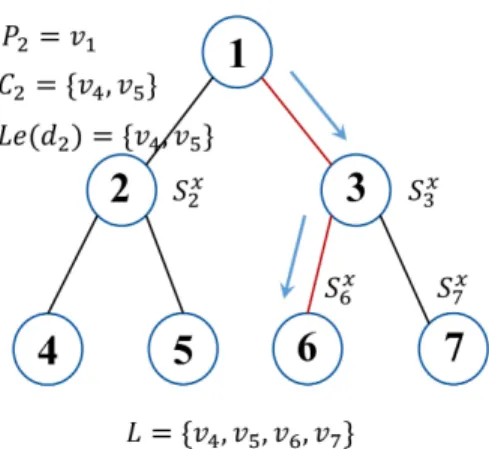
Fig. 1: Example of hierarchical tree structure and classification. The leaf node set of the tree is denoted asL={v4, v5, v6, v7}.For node
2, its parent node isP2=v1, its child nodes areC2={v4, v5}, and
its corresponding leaf nodes areLe(d2) ={v4, v5}. In a hierarchical
classification process, the samplexstarts at the root node1, and then is classified to the node with highest confidence score among all child nodesSx2 and S3x (assumeS3x> S2x). With proceeding this process
recursively, the prediction is node 6 for sample xin this example (assumeS6x> S7x).
(3) Transitivity: if vi ≺vj andvj ≺vk, then vi ≺vk for ∀vi, vj, vk∈ V;
Generally, there are several types of nodes in a tree hierar-chy. For node vi:
1) its parent node is denoted byPi;
2) its child nodes are denoted byCi, and|Ci|is the number
of child nodes of vi;
3) its ancestor nodes are denoted by Ω(vi), and|Ω(vi)| is the number of ancestor nodes ofvi;
4) its sibling nodes are denoted byΨ(vi)is the nodes which have the same parent node withvi;
5) its leaf nodes are denoted byLe(vi), and|Le(vi)|is the
number of leaf nodes ofvi. Specially,Ldenotes the leaf
nodes of the tree, and|L|denotes the number of all leaf nodes.
A toy example of the hierarchy can be seen in Fig. 1.
B. Hierarchical classification
Given a tree hierarchy, a classification task can proceed from the root to the leaves in a top-down manner. The widely used and most classical model is called a Pachinko Machine
[21], which classifies the samples starting from the root and choosing the child class with highest confidence recursively until a leaf class is reached.
Specifically, let x = {x1, x2, ..., xj, ..., xm} be a sample,
Wvibe a trained classifier called base classifier at nodevi, and Svxibe the confidence score given byWvi. Forx, the algorithm
will chooseCras the label at nodevi, whereSCxr = max(S
x
Ci).
See the toy example in Fig. 1. Assume a samplexstarts at the root nodev1, it first is assigned to the nodev3ifS3x> S2x. Then it will reach the leaf noded6 ifS6x> Sx7.
III. DEEPFUZZYTREELEARNING
In this section, we will introduce how to learn the tree structure and set the base classifiers for the deep learning
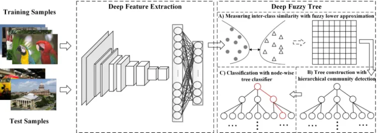
Fig. 2: Framework of Deep Fuzzy Tree. In the training phase, the deep features of training samples are first extracted, then inter-class similarities are measured and form similarity matrix in stepAfor tree construction, and a tree structure with base fuzzy rough classifiers is built by hierarchical community detection in stepB. In the test phase, after deep feature extraction step, test samples are assigned by fuzzy rough classifiers at each node of the tree from the root to the leaves (stepC).
model. In order to build a good tree structure, a proper inter-class similarity measurement is first designed and then applied for hierarchical community detection to form a tree. Given the tree structure, the base classifiers can be set on different nodes of the tree.
A. Measuring Inter-Class Similarity with Fuzzy Lower Ap-proximation
As shown in previous works, it is reasonable that classes with high visual similarity are grouped into one super-class [7], [14]. The key point in this issue lies in the proper measurement of similarity between different classes. Given the inter-class similarity matrix, clustering or community detection methods can be applied to build a tree. However, the designed mea-surements in previous works almost have some assumptions as discussed in Section I. Inspired by the theory of fuzzy rough sets, we propose a new measurement for better describing the similarity relations between different classes.
Given universe U representing a group of objects, let R be a fuzzy similar relation on U, with generated features B. Assume that R(x,y) monotonically decreases with the distance between x and y, and ∀x,y,z ∈ U, R has the following properties:
(1)R(x,x) = 1; (2)R(x,y) =R(y,x); (3)R(x,z)≥min
y (R(x,y), R(y,z)).
For any subsetX ⊂ hU, Ri, the lower approximation operator are defined as
RSX(x) = inf
y∈US(N(R(x,y)), X(y)) (1)
whereSrepresent fuzzy triangular conorm (T-conorm),N is a negator, and the standard negator is defined asN(x) = 1−x. Assume there have a set of classesY ={d1, d2, ..., di, ..., dN}.
For∀x∈U,di(x) =
0 , x /∈di 1 , x∈di
.
As proved by Moser and Bernhard [22], [23], givenTcos= max(ab−√1−a2√1−a2,0), kernel functions which have the property of reflexivity also have Tcos-transitive property.
Hence, givenU and kernel function k which have reflexivity and Tcos-transitive property, the fuzzy lower approximation
operator of fuzzy subset di ⊂U can be formulated as
kSdi(x) = inf
y∈US(N(k(x,y)), di(y)) = infy∈/di
(1−k(x,y))
(2) If we use Gaussian kernel to extract the relations in fuzzy rough calculations, the equation (2) is transformed into
kSdi(x) = inf y∈/di 1−exp −||x−y|| 2 σ . (3)
Equation (3) shows that the lower approximation membership degree ofxtodidepends on the nearest sample with different
label, since it needs to search the nearest sample in the space of U−di. Intuitively, the fuzzy lower approximation describes the
certain degree of a sample xbelonging to a specific classdi.
By considering the fuzzy lower approximation of all samples indi, the inter-class similarity can be measured appropriately. Definition 3.1: Given a set of samples(xi, yi), where xi ∈ {x1, ...,xm}, yi ∈ C = {C1, ..., Cn}, the fuzzy inter-class similarity(FIS) is defined as
K(Cab) = m X i=1 1 m inf xbi∈/Ca (1−k(xai,xbi)) , (4) where ∀xai, yai =Ca, ∀xbi, yai =Cb,
k(x, y) is the kernel function. Commonly, we use Gaussian kernel in the computation, so equation (4) turns into
K(Cab) = m X i=1 1 m inf xbi∈/Ca 1−exp −||xai−xbi|| 2 σ , (5)
Moreover, since the distance or similarity measurement should be symmetric intuitively, we define the dual fuzzy inter-class similarity (DFIS) as follows.
Definition 3.2:Dual fuzzy inter-class similarity is the aver-age of the bidirectional fuzzy inter-class similarity:
K(Ca, Cb) = 1
2(K(Cab) +K(Cba)). (6)
The similarity of each class pair is calculated according to equation (6), and then the similarity matrix of all labels can be obtained. Moreover, we prove theoretically that the proposed inter-class similarity obtains upper bounds to the generalization error bound of hierarchical classification (shown in section IV).
B. Tree Construction with Hierarchical Community Detection
With the proposed dual fuzzy class similarity, the inter-class similarity matrix is appropriately computed. Then the tree structure is obtained by grouping the more similar nodes as a granule recursively. Inspired by the community detection structure in the social network which reveals the organization of people (and its application to confusion graph (as pro-posed by Jin et al. [24]), we apply the adaptive modularity community detection algorithm hierarchically to explore the communities through the large number of classes. In contrast to the conventional use of spectral clustering, the adaptive modularity community detection methods automatically find the local optimal solution to the community modularities, without processing the similarity matrix to meet the needs of spectral clustering properties.
We utilize the fast community detection algorithm proposed by Blondel et al. [25], and extend it to hierarchical community detection. For the flat version of community detection, the key point is to compute the modularityQk of thekth community.
In our hierarchical scenario, we need to compute Qv
k at node
v in the tree structure Qvk= 1 2m X i,j (Si,j− kikj 2m)δ(ci, cj), (7) whereSi,jis the similarity degree of the edge between classi
and class j,ki=Pj(Sij)is the sum of similarity degrees of
the edges attached to the vertex class i,ci is the community
to which vertex class iis assigned, and the δ(p, q)function is 1 if p=qand 0 otherwise, and m= 12P
ijSij.
Then we follow the method of [25] which optimizes local modularity changes and the aggregated community at each node v, and apply the algorithm recursively to build the tree structure. In this way, we automatically compute the optimal number of communities at each node of the tree, which removes the need for the parameter setting of node numbers and tree depth in [14], [7].
However, using the aforementioned hierarchical community detection algorithm may sometimes generate a tree structure with few singleton nodes which have only one child node. We delete the redundant nodes in the constructed tree by using
T Npar(v) = Φv∈ν(π(v), µ(π(v)), (8)
Algorithm 1: Training Phase of Deep Fuzzy Ensemble Tree
Input: a set of training raw images(Xrtr= (xrtr, y),
wherexrtr={x1rtr,x 2 rtr, ...,x m rtr}, y={ytr1, ytr2, ..., ytrL}
Output: tree structure T, training images with deep featuresXf tr
1 Deep feature extraction and obtain Xf tr= (xf tr, ytr),
wherexf tr ={x1f tr,x
2
f tr, ...,x m f tr}. 2 // Obtain representative sample points; 3 fori= 1 :Ldo
4 GetrpSet(i) =Kmeans(xif tr(ytri 6=i), ritr); 5 // Construct affinity matrix.
6 fora= 1 : (L−1)do 7 forb= (a+ 1) :Ldo
8 ObtainK(Ca, Cb) according to (6); 9 // Perform hierarchical community detection in a
top-down process;
10 Initialize treeTinit with the root node; 11 TcurIter = CommunityDetect(Tinit); 12 TlastIter = Tinit;
13 while(TlastIter! =Tcuriter)do 14 TlastIter = TcurIter;
15 TcurIter = CommunityDetect(Tinit); 16 ifnum childNodes == 1 then 17 Node grandparent← Node child; 18 returnT =TcurIter,Xf tr.
whereπ(v)is the parent node of the current nodev,µ(π(v)) = 1if the number of child nodes of nodeπ(v)is greater than 1, and 0 otherwise. ForΦ(α, β), ifβ = 1, then it means there is no singleton nodes to be removed. In this case, letΦ(α, β) =
α. Otherwise,Φ(α, β) =β if node π(v) is a singleton node (µ(π(v)) = 0). In this case, we need to search the next parent node in ancestor node setν for nodev.
C. Classification with Node-Wise Tree Classifier
Given a learned tree structure T, a test sample needs to be assigned to one of the leaf nodes in the classification task. Similarly, we adopt the framework of classical Pachinko Machine to classify samples starting from the root node until a leaf node is reached. Consistent with the theory of fuzzy lower approximation utilized in measuring the inter-class similarity, we use the fuzzy rough classifier (FRC) as proposed by An et al. [26] as the base classifier, which assigns samples to the candidate class with the largest membership of the samples to the fuzzy lower approximation of the class. In other words, we utilize the lower approximation of samples to first measure the distance between classes appropriately, and then to assign the test samples to the right candidate class, which can help improve the overall performance. Moreover, using FRC as the base classifier of the tree can reduce the training time of the overall algorithm significantly as it does not need to be trained in advance before using in the test phase.
Algorithm 2: Test Phase of Deep Fuzzy Ensemble Tree Input: a set of test raw images (Xrts= (xrts, y), where
xrts={x1rts,x2rts, ...,xmrts},
y={yts1, yts2, ..., ytsL},
tree structure T
Output: PredictionsP Lof test data
1 Deep feature extraction and obtain Xf ts= (xf ts, yts),
wherexf ts={x1f ts,x
2
f ts, ...,x m f ts}.
2 // Perform hierarchical classification (Pachinko machine) withT, get P Li
ts.
3 forj= 1 :length(xrts)do 4 curN ode=root; 5 pcur=FRC(xjf ts, y
j
ts,xirts);while !ismember(pcur, leaf nodes)do 6 curN ode=pcur;
7 pcur=FRC(xjf ts, yjts,xirts); 8 P L(j) =pcur;
9 return P L,Xf tr.
D. Fast Adaptation to Large-Scale Tasks
Constructing the affinity matrix with all samples is time-consuming, especially for large-scale tasks. Therefore, in this paper, fast adaptation is proposed to solve this problem. With the aim of reducing sample numbers, vector quantization is used to generate a few representative points for each class. Although this method reduces the complexity remarkably, it does not lose much performance, as shown in our experiments. We will introduce vector quantization briefly in the following. Recall thatx∈ Xd is a sample ofd-dimensional vector, we
aim to obtain a reconstruction vector qi ∈ XC(1≤C ≤d)
through q = Q(x), where Q(·) is the quantization operator. Whenxis quantized asq, a distortion measured(·,·)can be defined betweenxandq. The overall average distortion with m samples is written as Dt = m1
Pm i=1
PC
j=1d(xi,qi). To
split the original space intoC cells, each cellCi is associated
with a reconstruction vectorqi.
We use mean square error (mse)d(x,q) = N1 PNk=1kxk−
qkk2 as the distortion measurement, and this process turns to
the well-known K-means algorithm. Representative pointsrCi
are generated for each class Ci by setting a proportion η of
samples in the class. Note that at least one representative point is ensured for each class.
With the aforementioned parts, we summarize the proposed deep fuzzy tree model. In the training phase, deep features are first extracted and the inter-class similarity are measured based on the features of training samples, then hierarchical community detection is applied to build a tree structure (see Algorithm 1). In the test phase, after feature extraction, test samples are assigned by the fuzzy rough set classifier at each node of the tree structure (see Algorithm 2).
IV. THEORETICALRESULTS
To find the rationality and features of the proposed model, we analyze the generalization error bound of hierarchical
classification, and prove theoretically that the designed fuzzy inter-class similarity can help improve the performance of hierarchical classification in the following proposition.
Proposition 1: Let S = (xi, yi)ni=1 be a set of samples drawn i.i.d. based on a probability distributionDoverX × Y. Let Λ(xi, y) be the membership of xi to class y, and Φ(Λ)
be the kernel function for Λ. Given a tree structure T, the empirical data-dependent error of hierarchical classification with HerrS[f] is upper bounded by the fuzzy inter-class
similarityK(S).
Proof: Rademacher complexity is widely used to analyze the generalization error bound of a classification problem [27]. We utilize the theorem presented by Shawe et al. [28] for Rademacher data-dependent generalization bound in this issue
HerrD[f]≤\HerrS[f] + 2Rbm(G(F)) + 3 r
ln(2/δ)
m , (9) where F is a set of hypotheses, HerrD(f)) = ED[f]
represents the generalization error of a hierarchical classifier, and \HerrS[f] = EbS[f] represents the empirical error of a
hierarchical classifier, with the minimum probability of1−δ. In the scenario of hierarchical classification, we definef ∈ F as
F={f : (x, y)∈ X × Y 7→ hΛ(x, y),Φ(Λ)i}, (10) whereΛ(x, y)is the membership of xto class y, and Φ(Λ)
is the kernel function forΛ.
Babbar et al. [5] have presented the generalization error bound of hierarchical classification with kernel classifiers. In-spired from their work, we focus on the Radamecher complex-ity term to explore the influence of inter-class measurement as
ˆ Rm(G(F)) =Eσ " sup gf∈GF 1 m m X i=1 σigf(xi, yi) # =Eσ " sup gf∈GF 1 m m X i=1 σi min v∈Φ(yi) (f(xi, v)− max v0∈Ψ(v)f(xi, v 0)) # , (11) where σis are Rademacher variables which are independent
uniform random variables whose values are chosen from set
{−1,+1}. Here we utilize the definition of Babbar et al. [5] for hierarchical classification, which develops the multi-class margin in [29] as G(F)) ={gf :(x, y)∈ X × Y 7→ min v∈Φ(yi) (f(xi, v)− max v0∈Ψ(v)f(xi, v 0))|f ∈ F } (12) Then equation (11) can be transformed with the construction of cas ˆ Rm(G(F)) ≤Eσ sup gf∈GF X (v,v0)∈Y2 v0∈Ψ(v) 1 m X i∈C σi(f(xi, v)−f(xi, v0)) , (13) where i= [1,2, ..., m], C:c(f,xi, yi) = (v, v0).
As∀i, j∈ {l|c(f,xl, yl) = (v, v0)}2, i6=j,Eσ[σi, σj] = 0,
inequality (13) can be relaxed according to Jensen’s inequality as follows: ˆ Rm(G(F)) ≤ 1 mgfsup∈GF X (v,v0)∈Y2 v0∈Ψ(v) Eσ X i∈C σi(f(xi, v)−f(xi, v0)) !2 1 2 = 1 mgfsup∈GF X (v,v0)∈Y2 v0∈Ψ(v) X i∈C (f(xi, v)−f(xi, v0)) = 1 mgfsup∈GF X (v,v0)∈Y2 v0∈Ψ(v) X i∈C (hΛxi, v),Φ(Λ)i − hΛxi, v0),Φ(Λ)i) (14) If we take the membership function as the lower approxima-tion and take the kernel funcapproxima-tion as Gaussian kernel, inequality (14) is in the form of 1 mgfsup∈GF X (v,v0)∈Y2 v0∈Ψ(v) X i∈C inf ˆ xv∈v 1−exp −||xi−xˆv|| 2 σ − inf ˆ xv0∈v0 1−exp −||x−xˆv0|| 2 σ = 1 mgfsup∈GF X (v,v0)∈Y2 v0∈Ψ(v) X i∈C (Kxi(Cv)− Kxi(Cv0)) ≤ sup gf∈GF X (v,v0)∈Y2 v0∈Ψ(v) X i∈C Kxi(Cv, Cv0) m (15) where the node vis the ground truth node, and the nodev0 is the other node which is the most similar node with respect to the a certain samplexi.
Inequality (15) shows that for the sample xi ∈ S, the
generalization upper bound is influenced by the fuzzy inter-class similarity between node v and v0. For each node in the tree, the error upper bound will be smaller if the fuzzy inter-class similaritybetween the ground truth node and other sibling nodes is larger. In the proposeddeep fuzzy treemodel, we realize inequality (15) by clustering the classes based on the inter-class matrix with respect to the fuzzy inter-class similarity to maintain large inter-class similarity at each non-leaf node. The proposition also demonstrates that settingFRC
as the base classifier can further improve the classification performance along with the tree structure built upon fuzzy
inter-class similarity.
V. EXPERIMENTS
A. Dataset and Implementations
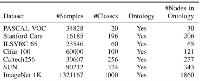
We perform experiments on various datasets (See Table I). Typically, these datasets are all organized by using a semantic tree structure, which shows the hierarchical relations between classes.
TABLE I: Dataset description.
#Nodes in Dataset #Samples #Classes Ontology Ontology
PASCAL VOC 34828 20 Yes 30
Stanford Cars 16185 196 Yes 206
ILSVRC 65 23546 60 Yes 65
Cifar 100 60000 100 Yes 121
Caltech256 30607 256 Yes 277
SUN 90212 324 Yes 343
ImageNet 1K 1321167 1000 Yes 1860
• PASCAL VOC [30]: a visual object classes dataset which is a benchmark in visual object category recognition and detection. It has 34828 images with 20 classes.
• ILSVRC65 [31]: a visual object image dataset which is the subset of ImageNet. It has 17100 samples in 65 different classes.
• Stanford Cars [32]: a car image dataset which aims to address the fine-grained classification problem. It has 16185 samples in 196 different classes.
• Cifar-100 [33]: an image dataset containing 60000 sam-ples in 100 classes, with 600 images in each class. • Caltech256 [34]: an image dataset with various types of
classes. It has 30607 image samples and 256 class labels. • SUN [35]: a scene understanding dataset with 397 kinds of scenes. We modify it by leaving out the categories that have more than one parent labels and samples with multiple labels. Finally SUN dataset turns into 324 classes with at least 100 images per category.
• ImageNet 1K [36]: a large-scale image classification dataset which contains 1000 categories.
Each dataset is split into a training subset and a test subset by 80%, 20%, respectively. The training subset is used to construct the hierarchical structure, while the test subset is used to obtain the classification results. All the results shown are the average of 5-time running results, and all the experiments are executed on an Intel Core i7-600 running the Windows 8 operating system at 3.40 GHz with 32 GB memory.
B. Comparison Methods
We compare various algorithms including tree construction, semantic ontology and deep learning baseline model.
• Label Tree (LT) [12]: builds the label tree based on the confusion degree of classification results. It first learns a multiclass SVM and gets the confusion matrix through classification as the affinity matrix. Then the tree is built through hierarchical spectral clustering method.
• Mean-Vector Based Tree Learning (MeanVT) [14]: con-siders the distance between the center of different classes as the distance between different classes and hence builds the similarity matrix. Then it uses hierarchical spectral clustering to build the tree according to the similarity matrix.
• Mean-Variance based Visual Tree Construction (Mean-VarVT) [7]: constructs a similarity matrix by using the mean vector and the variance vector of each class to measure the distance between different classes. Then
TABLE II: Classification accuracy as a percentage, with rank shown in parentheses. The best result obtained for each dataset is highlighted in bold.
Datasets Standard VGG Ontolgy LabelTree MeanVT MeanVarVT EnhancedVT DFT PASCAL VOC 75.55 (1) 73.40 (7) 74.66 (4) 74.50 (5) 73.43 (6) 75.19 (3) 75.51 (2) ILSVRC 65 85.70 (3) 85.64 (4) 86.68 (2) 85.30 (7) 85.40 (6) 85.42 (5) 87.27 (1) Stanford Cars 58.13 (2) 51.74 (6) 55.15 (3) 51.00 (7) 52.30 (5) 52.51 (4) 59.90 (1) Cifar 100 72.72 (1) 70.09 (4) 70.89 (3) 68.91 (5) 67.72 (7) 68.68 (6) 72.53 (2) Caltech 256 82.11 (3) 80.54 (7) 81.31 (5) 81.17 (6) 82.19 (2) 81.61 (4) 82.67 (1) SUN 82.91 (2) 81.25 (6) 82.05 (3) 81.28 (5) 80.93 (7) 81.67 (4) 84.41 (1) ImageNet 1K 61.98 (2) 60.55 (5) 60.56 (4) 60.45 (7) 60.50 (6) 61.90( 3) 62.11 (1) Avg. Rank 2.000 5.571 3.000 6.000 6.000 4.143 1.286
it uses hierarchical spectral clustering to build a tree according to the similarity matrix.
• Enhanced Visual Tree Construction (EnhancedVT) [8]: first proceeds through active sampling to choose a small part of samples reflecting the features of the dataset, then applies Hasudorff distance to construct the affinity matrix. Finally it utilizes hierarchical spectral clustering method to build the label tree structure.
• Ontology (OTG): is the expert-designed semantic tree structure. It reflects the thinking manner of human beings and helps organize the datasets.
• Standard VGG Net [6]: is the conventional VGG deep learning model, which uses softmax layer to classify the sample to all the candidate classes in a flat manner. We use pre-trained VGG-19 Net fine-tuned with various datasets in this paper for deep feature extraction, and replace its softmax layer with the proposed deep fuzzy tree algorithm.
For fair comparison with the quality of the tree structure fairly, we obtain the different inter-class relation matrix and apply the same community detection method to build the tree structure for [12], [14], [7], [8].
C. Results on Classification Performance
In order to investigate the performance of the proposed model, we compare DFT with other state-of-the-art models on six visual datasets, and use classification accuracy of the original test labels to assess the performance. In the proposed
DFT, we set parameter η = 0.05, and choose the best parameterσfrom the candidate set{10−2,10−1, ...,106}. The results are shown in Table II.
There are three aspects of these results that merit discussion. First, flat classification versus hierarchical classification. Table II shows that Standard VGG-19 Net performs well in datasets without too many labels in comparison with all hierarchical methods, such as PASCAL VOC, ILSVRC 65 and Cifar 100. Just as [4] and [5] pointed out, flat classifier performs better in the easy tasks while a hierarchical classifier is good at handling some difficult tasks by dividing the hard task into many easier subtasks. DFT outperforms the flat VGG-19 Net in most of the datasets with a large number of more labels, which verifies the conclusion of [4] and [5].
Second, ontology versus data-driven hierarchy. Table II demonstrates that ontology-based method performs well in ILSVRC 65, Cifar 100 and SUN in comparison with data-dependent hierarchical methods except DFT, which suggests
that human knowledge is very helpful for determining structure and classification. However, there are large gaps between ontology-based and data-dependent hierarchical methods in PASCAL VOC and Stanford Cars. This suggests that building the tree structure without data does not work well in all the classification tasks, as a semantic gap exists in these tasks which needs to be improved by considering data information. Third, different hierarchical structure learning algorithms. It can be seen from Table II that our proposedDFTperforms bet-ter than other hierarchical methods in all the datasets.MeanVT
generally fails to get a good performance since utilizing one central point to represent all the samples can hardly express all information in data, and will only be effective if the data distributions of all the classes are ball-shaped. MeanVarTC
improves this problem by using the mean and variance of data, thereby improving performance noticeably. However, it also has a prior assumption that the data distribution is Gaussian, which is often the case, but is hard to verify for data distributions of massive classes. In contrast, the performance of EnhancedVT in datasets with fewer labels is generally better than in datasets with massive labels. The limit for this algorithm is that Hausdorff distance is sensitive to abnormal points, and this is inevitably in datasets with massive labels. Finally, although theLabelTree algorithm performs relatively well in various datasets, it cannot ensure the reliability of SVM for all the datasets, especially for those with huge amounts of labels.
Moreover, to further explore whether the observed dif-ferences are statistically significant, the Friedman test [37] for multiple comparisons, together with the Bonferroni-Dunn post-hoc test [38] to identify pairwise differences, are applied on the all seven datasets. In the Friedman test, given k compared algorithms and N datasets, let rij be the rank of the jth algorithm on the ith dataset, and Ri = N1 PNi=1rji
be the average rank of algorithm i among all datasets. The null-hypothesis of Friedman test is that all the algorithms are equivalent in terms of classification accuracy. Under null-hypothesis, the Friedman statistic is distributed according to χ2F withk−1degrees of freedom
χ2F = 12N k(k+ 1) k X i=1 R2i −k(k+ 1) 2 4 ! FF = (N−1)χ2 F N(k−1)−χ2 F , (16)
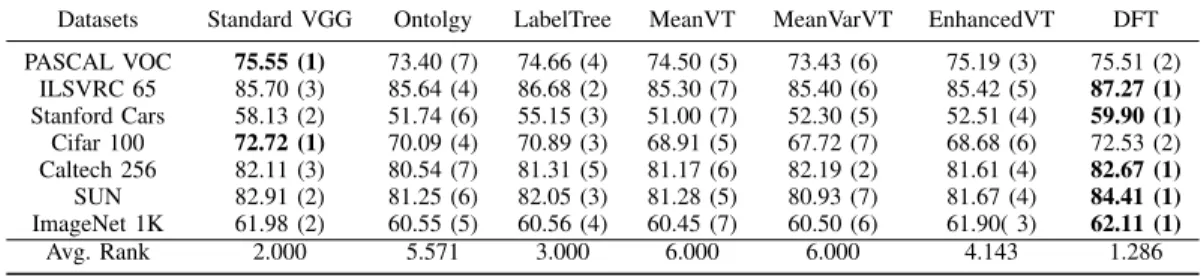
(a) Expert-designed semantic tree structure. (b) Tree structure learned by the proposedDFTalgorithm.
Fig. 3: Tree structures comparison on PASCAL VOC dataset. The learned tree structure groups class with similar shape (BirdandAeroplane,
TrainandBus) into one super-class, which reflects the visual feature similarity of various classes in the dataset better.
Fig. 4: Classification accuracy comparison ofDeep Fuzzy Treeagainst the other algorithms with the Bonferroni-Dunn test.
Fig. 5: Classification accuracy comparison ofDeep Fuzzy Treeagainst
Standard VGGwith the Bonferroni-Dunn test.
(k−1)(N −1) degrees of freedom. The average rank of all the algorithms in terms of classification accuracy is listed in Table II, and the valueFF = 26.649is computed according to
equation (16). With seven algorithms and seven datasets, the critical value for α= 0.05 of F((7−1),(7−1)×(7−1))
is 2.3638, so the null-hypothesis can be rejected. Thus, all the algorithms are not equivalent in terms of classification accuracy, and there exist significant differences between them. Then the Bonferroni-Dunn post-hoc test is leveraged to detect if the DFT algorithm is better than the existing ones on the all seven datasets. Specifically, the performance of the two compared algorithms are significantly different if the distance between the averaged ranks exceeds the critical
distance (CD): CDα = qα q
k(k+1)
6N , where qα is given in
Table 5 of [39]. Note that q0.1 = 2.394 with k = 7, so CD0.1=q0.1
q
7×8
6×7. Fig. 4 visually shows the CD diagrams in terms of classification accuracy, in which the lowest (best) ranks appear on the right of the x-axis. The bars show the estimated range of ranks, such that algorithms for which the bars do not overlap horizontally are statistically different. From Fig. 4, therefore, in terms of classification accuracy,
DFT performs statistically better than MeanVT, MeanVarVT, OntologyandEnhancedVT, but there is no statistical difference between DFT, Standard VGG and LabelTree. According to conclusion of [4], [5] and TABLE II,DFT is more appropriate to deal with data with a large number of labels thanStandard VGG, so we do another Bonferroni-Dunn test of DFT and
Standard VGG across four datasets with many labels, i.e.,
Stanford Cars, Caltech 256, SUN and ImageNet 1K. In this test, q0.1 = 1.645 with k = 2 leads to CD0.1 = 0.8225. The result is shown in Fig. 5 and demonstrates that there exists statistical difference betweenDFT andStandard VGG, which verifies that DFT performs better than Standard VGG
in datasets with a large number of labels.
D. Case Study on Learned Tree Structures
To better understand the features of structures, we analyze and visualize the PASCAL VOC dataset in Fig. 3. Fig. 3(a) is the expert-designed semantic structure, and Fig. 3(b) is the structure learned by DFT. There are some slight differences between these two structures, which are annotated in red. In the semantic structure, Aeroplane and Bird belong to superclass Vehicles and Animal respectively. However, they are grouped into the same superclass in the structure learned byDFT. Actually the images ofAeroplaneandBird are very similar in visualization, and it is more reasonable to group them into one superclass. Similarly, Bus is the fine-grained
TABLE III: Running time (s) of tree construction in four datasets.
Datasets LabelTree MeanVT MeanVarVT EnhancedVT DFT PASCAL VOC 140(4) 49(1) 57(3) 142(5) 56(2) ILSVRC 65 125(5) 38(1) 50(3) 110(4) 42(2) Stanford Cars 189(4) 33(1) 58(2) 247(5) 64(3) Cifar 100 1218(4) 339(1) 614(2) 1861(5) 887(3) Caltech 256 769(5) 250(1) 371(3) 563(4) 352(2) SUN 2501(4) 930(1) 1604(3) 5693(5) 1143(2) ImageNet 1K 400932(5) 93941(1) 131941(2) 282236(4) 133716(3) Avg. Rank 4.429 1.000 2.571 4.571 2.429
Fig. 6: Visualization of the learned tree structures. The learned tree structure removes the classMushroomfrom the groupFruit and Vegetables, which corrects the unreasonable local parts of the semantic tree structure addressed by [33].
class of 4-Wheeled VehicleswhereasTrainis not. In contrast, they are assigned to the same superclass in the structure learned by DFT. It is shown that the images of Train are almost locomotive images, which has a lot of resemblance with the images of Bus, hence it is more reasonable to group them together.
Moreover, we visualize the learned tree structures of Cifar 100 datasets in Fig. 6, and it can be explicitly shown that the relations between different classes are deeply connected. It is worth noting that the learned structure corrects mistakes in the original human-designed structure. As stated in [33], Mush-room is grouped into Fruit and Vegetables for convenience, but they really do not belong to that group. Our learned tree structure correctly placesMushroominto a separate new group, as shown in Fig. 6.
Fig. 7: Comparison on running time of tree construction phase betweenDeep Fuzzy Treeand other algorithms with the Bonferroni-Dunn test.
E. Results on Efficiency of Tree Construction
To explore the efficiency of our algorithm, we run all the hierarchical models on all seven datasets and compare the
run-(a)σ= 100 (b)σ= 1000 (c)σ= 10000
Fig. 8: Analysis of parameterη with differentσs.
(a)η= 0.05 (b)η= 0.15 (c)η= 0.25
Fig. 9: Analysis of parameterσ with differentηs.
ning time of tree construction, including LabelTree, MeanVT, MeanVarVT, EnhancedVT andDFT.Ontology method uses a pre-defined tree structure constructed by humans andStandard VGG does not make use of a tree structure, so they are not included in this part of the experiments. ForDFT, we set the parameterη= 0.05. The results are shown in Table III. It can be seen that MeanVT is the most efficient algorithm, while
EnhancedVT takes the longest time to build the tree. The efficiency of the proposed DFT generally comes just behind
MeanVT and is comparable toMeanVarVT. To further explore the statistical differences, the Friedman test and Bonferroni-Dunn post-hoc test are again applied. In the Friedman test, the null-hypothesis is that all the tree learning algorithms are considered equivalent in terms of run time. According to equation (16), χ2
F = 22.456 and FF = 24.303 with
five tree learning algorithms and seven datasets. Therefore, we can reject the null-hypothesis and conclude that there are significant differences between the algorithms. With the rejection of the null-hypothesis, the Bonferroni-Dunn post-hoc test can be proceeded to explore if the algorithms are compared to each other. In this case, it is used to explore if the proposed algorithm is statistically better than others.
The Bonferroni-Dunn post-hoc test result is shown in Fig. 7 with the CD diagrams in terms of run time. From this, we can conclude that the proposed DFT is comparable with MeanVT
andMeanVarVT, with no statistical differences between them. However, LabelTree andEnhancedVT are not so efficient in comparison with these three algorithms.LabelTreefirst trains a multiclassSVMand then uses it to get the confusion matrix, so the efficiency is heavily influenced by the training ofSVM.
EnhancedVT aims to find the most important samples for data, requiring large amounts of time to get the selected sample set.
The reason forEnhancedVTbeing less efficient thanLabelTree
in some datasets is mainly due to the process of selecting sample set in terms of computing multiple features of data, which takes up most of the running time. It is worth noting that LabelTree and EnhancedVT perform well in the cost of decrease in efficiency. On the other hand, MeanVT and
MeanVarVTalgorithm are very efficient, but their performance is not as good as other hierarchical methods since they cannot measure the similarity between classes accurately by assuming data distribution as ball-shaped or Gaussian. The proposed
DFT obtains the best level (withLabelTree) of classification accuracy whilst its efficiency is comparable with MeanVT MeanVarVT and StandardVGG, which indicates thatDFT is both effective and efficient.
F. Parameter Analysis
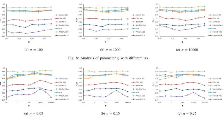
There are two parameters in the proposed model, σ and η. To explore the influence of each parameter, various combinations are explored in this experiment. We choose σ ranging from {10−2,10−1, ...,104} and η ranging from
{0.05,0.15, ...,0.65}. Generally, we investigate influence of different combination ofσandη on classification accuracy in Fig. 8, Fig. 9 and Fig. 9-14 (see in Supplemental Material), where Fig. 8 and Fig. 9 show some recommended choices of the parameters and Fig. 9-14 describe the influence of all the alternatives for the parameters.
Firstly,ηis the ratio of representative samples in each class, and the largerη is, the more original information of the data contains. Fig. 8 shows that the classification accuracy first increases from η = 0.05 and then decreases until η = 0.45. This indicates that even though using more samples is helpful for training the model, inappropriate ratios of representative
points will lead to a decrease in performance. The reason may be that the general features of data can be partly reflected by few representative points but gradually being better until there are sufficient points to describe the overall features. Moreover, a larger value ofη can help improve performance since more information of data is leveraged. Interestingly, η = 0.05
appears to be a good choice for balancing the effectiveness and efficiency experimentally, which indicates that small data can also produce good results if they can reflect the general information of the dataset properly.
Secondly, Fig. 9 shows that the optimal (or near-optimal) value of σ is different for various datasets. With the fixed value of η, values ofσ in the range [102,104] achieve good performance in most datasets. Furthermore, we also plot all the combination of η and σ to explore more details of the parameter influence in Fig. 9-14 of Supplemental Material. Generally, we find that the classification accuracy is broadly similar when each parameter has a value in the recommended interval, but there are significant differences if inappropriate values of the parameters are selected.
VI. CONCLUSION
In this paper, we propose a new deep fuzzy tree (DFT) framework, aiming at gaining the benefit from hierarchical classification to help deep learning solve classification tasks with large numbers of labels. With the help of the theory of fuzzy rough sets, dual fuzzy inter-class similarityis designed to learn a better tree structure along with setting fuzzy rough classifier as the base classifier. It is further proved theoretically to be effective for hierarchical classification. By using com-munity detection methods, a tree structure can be constructed by hierarchically detecting the most similar communities. To deal with large scale tasks, fast adaptation is designed by using vector quantization. The performance of the proposed DFT
algorithm shows the effectiveness and efficiency in comparison with the standard deep learning model and state-of-the-art hierarchical classification models.
REFERENCES
[1] C. Spampinato, S. Palazzo, I. Kavasidis, D. Giordano, N. Souly, and M. Shah, “Deep learning human mind for automated visual classifica-tion,”IEEE Conference on Computer Vision and Pattern Recognition, pp. 4503–4511, 2017.
[2] N. Lu, T. Li, X. Ren, and H. Miao, “A deep learning scheme for motor imagery classification based on restricted boltzmann machines,”IEEE Transactions on Neural Systems and Rehabilitation Engineering, vol. 25, no. 6, pp. 566–576, 2017.
[3] H. Zhao, P. Zhu, P. Wang, and Q. Hu, “Hierarchical feature selection with recursive regularization,”International Joint Conference on Artifi-cial Intelligence, pp. 3483–3489, 2017.
[4] R. Babbar, I. Partalas, E. Gaussier, and M. R. Amini, “On flat ver-sus hierarchical classification in large-scale taxonomies,”International Conference on Neural Information Processing Systems, pp. 1824–1832, 2012.
[5] I. Partalas, I. Partalas, E. Gaussier, and M. R. Amini, “Learning taxonomy adaptation in large-scale classification,”Journal of Machine Learning Research, vol. 17, no. 1, pp. 3350–3386, 2016.
[6] K. Simonyan and A. Zisserman, “Very deep convolutional networks for large-scale image recognition,”arXiv preprint arXiv:1409.1556, 2014. [7] Y. Qu, L. Lin, F. Shen, and et al., “Joint hierarchical category structure
learning and large-scale image classification,” IEEE Transactions on Image Processing, vol. 26, no. 9, pp. 4331–4346, 2017.
[8] Y. Zheng, J. Fan, J. Zhang, and X. Gao, “Hierarchical learning of multi-task sparse metrics for large-scale image classification,” Pattern Recognition, vol. 67, pp. 97–109, 2017.
[9] O. Russakovsky, J. Deng, H. Su, and et al., “Imagenet large scale visual recognition challenge,”International Journal of Computer Vision, vol. 115, no. 3, pp. 211–252, 2015.
[10] M. Sun, W. Huang, and S. Savarese, “Find the best path: An efficient and accurate classifier for image hierarchies,”IEEE International Conference on Computer Vision, pp. 265–272, 2014.
[11] G. Griffin and P. Perona, “Learning and using taxonomies for fast visual categorization,”IEEE Conference on Computer Vision and Pattern Recognition, pp. 1–8, 2008.
[12] S. Bengio, J. Weston, and D. Grangier, “Label embedding trees for large multi-class tasks,”In Advances in Neural Information Processing Systems, pp. 163–171, 2013.
[13] B. Liu, F. Sadeghi, M. Tappen, O. Shamir, and C. Liu, “Probabilistic la-bel trees for efficient large scale image classification,”IEEE Conference on Computer Vision and Pattern Recognition, pp. 843–850, 2013. [14] J. Fan, J. Peng, L. Gao, and N. Zhou, “Hierarchical learning of tree
classifiers for large-scale plant species identification,”IEEE Transactions on Image Processing, vol. 24, no. 11, pp. 4172–4184, 2015.
[15] P. Dong, K. Mei, N. Zheng, H. Lei, and J. Fan, “Training inter-related classifiers for automatic image classification and annotation,” Pattern Recognition, vol. 46, no. 5, pp. 1382–1395, 2013.
[16] Q. Hu, L. Zhang, Y. Zhou, and W. Pedrycz, “Large-scale multimodality attribute reduction with multi-kernel fuzzy rough sets,”IEEE Transac-tions on Fuzzy Systems, vol. 26, no. 1, pp. 226–238, 2018.
[17] A. Tan, W. Z. Wu, Y. Qian, J. Liang, J. Chen, and J. Li, “Intuitionistic fuzzy rough set-based granular structures and attribute subset selection,”
IEEE Transactions on Fuzzy Systems, 2018.
[18] F. Feng, H. Fujita, M. I. Ali, R. R. Yager, and X. Liu, “Another view on generalized intuitionistic fuzzy soft sets and related multiattribute decision making methods,”IEEE Transactions on Fuzzy Systems, 2018. [19] C. N. S. Jr and A. A. Freitas, “A survey of hierarchical classification across different application domains,”Data Mining & Knowledge Dis-covery, vol. 22, pp. 31–72, 2011.
[20] K. Aris, P. Ioannis, G. Eric, G. Paliouras, and I. Androutsopoulos, “Evaluation measures for hierarchical classification: A unified view and novel approaches,”Data Mining & Knowledge Discovery, vol. 29, no. 3, pp. 820–865, 2015.
[21] D. Koller and M. Sahami, “Hierarchically classifying documents us-ing very few words,”International Conference on Machine Learning, vol. 97, pp. 170–178, 1997.
[22] B. Moser, “On the t-transitivity of kernels,”Fuzzy Sets and Systems, vol. 157, no. 13, pp. 1787–1796, 2006.
[23] B.Moser, “On representing and generating kernels by fuzzy equivalence relations,” Journal of Machine Learning Research, vol. 7, pp. 2603– 2620, 2006.
[24] R. Jin, Y. Dou, Y. Wang, and X. Niu, “Confusion graph: Detecting confusion communities in large scale image classification,”Twenty-Sixth International Joint Conference on Artificial Intelligence, pp. 1980–1986, 2017.
[25] V. D. Blondel, J. L. Guillaume, R. Lambiotte, and E. Lefebvre, “Fast unfolding of communities in large networks,” Journal of Statistical Mechanics, vol. 2008, no. 10, pp. 155–168, 2008.
[26] S. An, Q. Hu, and D. Yu,Case-Based Classifiers with Fuzzy Rough Sets. Springer Berlin Heidelberg, 2011.
[27] P. L. Bartlett and S. Mendelson, “Rademacher and gaussian complexi-ties: Risk bounds and structural results,”Journal of Machine Learning Research, vol. 3, pp. 463–482, 2003.
[28] J. Shawe-Taylor and N. Cristianini,Kernel Methods for Pattern Analysis. Publications of the American Statistical Association, 2004.
[29] Y. Guermeur, “Sample complexity of classifiers taking values in rq, application to multi-class svms,” Communications in StatisticsTheory and Methods, vol. 39, no. 3, pp. 543–557, 2010.
[30] M. Everingham, L. V. Gool, and W. et.al., “The pascal visual object classes (voc) challenge,” International Journal of Computer Vision, vol. 88, no. 2, pp. 303–338, 2010.
[31] D. Jia, “Hedging your bets: Optimizing accuracy-specificity trade-offs in large scale visual recognition,”IEEE Conference on Computer Vision and Pattern Recognition, pp. 3450–3457, 2012.
[32] J. Krause, M. Stark, D. Jia, and F. F. Li, “3d object representations for fine-grained categorization,”IEEE International Conference on Comput-er Vision Workshops, pp. 554–561, 2014.
[33] A. Krizhevsky, “Learning multiple layers of features from tiny images,”
Tech Report, Department of Computer Science, University of Toronto, 2009.
[34] G. Griffin, A. Holub, and P. Perona, “Caltech-256 object category dataset,”California Institute of Technology, 2007.
[35] J. Xiao, J. Hays, and K. A. e. Ehinger, “Sun database: Large-scale scene recognition from abbey to zoo,”Computer Vision and Pattern Recognition, pp. 3485–3492, 2010.
[36] O. Russakovsky, J. Deng, H. Su, J. Krause, S. Satheesh, S. Ma, Z. Huang, A. Karpathy, A. Khosla, M. Bernstein, A. C. Berg, and L. Fei-Fei, “Imagenet large scale visual recognition challenge,”International Journal of Computer Vision, vol. 115, no. 3, pp. 211–252, 2015. [37] M. Friedman, “A comparison of alternative tests of significance for the
problem of m rankings,”The Annals of Mathematical Statistics, vol. 11, no. 1, pp. 86–92, 1940.
[38] O. J. Dunn, “Multiple comparisons among means,” Journal of the American Statistical Association, vol. 56, no. 293, pp. 52–64, 1961. [39] J. Demˇsar, “Statistical comparisons of classifiers over multiple data sets,”
Journal of Machine Learning Research, vol. 7, pp. 1–30, 2006.
Yu Wangreceived the B.S. degree in communica-tion engineering and the M.S. degree in software engineering from Tianjin University in 2013 and 2016, respectively, where he is currently the Ph.D. candidate with the School of Computer Science and Technology. His research interests focus on hierarchical learning and image classification in data mining and machine learning.
Qinghua Hu received the B.S., M.S., and Ph.D. degrees from the Harbin Institute of Technology, Harbin, China, in 1999, 2002, and 2008, respec-tively. He was a Post-Doctoral Fellow with the Department of Computing, Hong Kong Polytechnic University, from 2009 to 2011. He is currently the Dean of the School of Artificial Intelligence, the Vice Chairman of the Tianjin Branch of China Computer Federation, the Vice Director of the SIG Granular Computing and Knowledge Discovery, and the Chinese Association of Artificial Intelligence. He is currently supported by the Key Program, National Natural Science Foundation of China. He has published over 200 peer-reviewed papers. His current research is focused on uncertainty modeling in big data, machine learning with multi-modality data, intelligent unmanned systems. He is an Associate Editor of the IEEE TRANSACTIONS ON FUZZY SYSTEMS, Acta Automatica Sinica, and Energies.
Pengfei Zhureceived the Ph.D. degree in computer vision from The Hong Kong Polytechnic University, Hong Kong, China, in 2015. He received his B. S. and M. S. in power engineering and power machinery and engineering respectively from Harbin Institute of Technology, Harbin, China in 2009 and 2011, respectively. Now he is an associate professor with the College of Intelligence and Computing, Tianjin University. His research interests are focused on machine learning and computer vision. He has published more than 30 papers in ICCV, CVPR, ECCV, AAAI, IJCAI, and IEEE TIFS, TYC, TIP. He is the local arrangement chair of IJCRS 2015, CCML 2017 and CCCV 2017.
Linhao Li received the B.S. degree in applied mathematics, the M.S. degree in computational mathematics and PhD degree in computer science from Tianjin University in 2012, 2014 and 2019 respectively. Now he is currently working as an assistant professor in School of Artificial Intelligent in Heibei University of technology. His research interests focus on quantization and hashing learning, sparse signal recovery, background modeling, and foreground detection.
Bingxu LuBingxu Lu received B. S. degree from Nanjing Agriculture University, Nanjing, China in 2016. Now he is a PhD candidate with College of Intelligence and Computing. His research interests are focus on deep learning and computer vision.
Jonathan M. Garibaldireceived the B.Sc (Hons) degree in Physics from Bristol University, UK in 1984, and the M.Sc. degree in Intelligent Systems and the Ph.D. degree in Uncertainty Handling in Immediate Neonatal Assessment from the University of Plymouth, UK in 1990 and 1997, respectively. He is Head of School of Computer Science at the University of Nottingham, UK, and leads the Intelligent Modelling and Analysis (IMA) Research Group. The IMA research group undertakes research into intelligent modelling, utilising data analysis and transformation techniques to enable deeper and clearer understanding of complex problems. His main research interests are modelling uncertainty and variation in human reasoning, and in modelling and interpreting complex data to enable better decision making, particularly in medical domains. He has made many theoretical and practical contributions in fuzzy sets and systems, and in a wide range of generic machine learning techniques in real-world applications. Prof. Garibaldi has published over 200 papers on fuzzy systems and intelligent data analysis, and is the Editor-in-Chief of IEEE Transactions on Fuzzy Systems (2017-). He has served regularly in the organising committees and programme committees of a range of leading international conferences and workshops, such as FUZZ-IEEE, WCCI, EURO and PPSN. He is a member of the IEEE.
Xianling Li received his B. S., M. S. and Ph.D. degrees from Harbin Institute of Technology, Harbin, China in 2005, 2007 and 2011, respectively. Now he is a senior engineer at Science and Technology on Thermal Energy and Power LaboratoryWuhan, China. His interests are focused on big data, fault diagnosis of complex power system, intelligent con-trol.
![Fig. 6: Visualization of the learned tree structures. The learned tree structure removes the class Mushroom from the group Fruit and Vegetables, which corrects the unreasonable local parts of the semantic tree structure addressed by [33].](https://thumb-us.123doks.com/thumbv2/123dok_us/380197.2542027/9.918.109.814.94.730/visualization-structures-structure-mushroom-vegetables-unreasonable-structure-addressed.webp)