Positive Integral Operators With Analytic Kernels

Journal of Arts and Sciences Say›: 6 / Aral›k 2006

Positive Integral Operators With

Analytic Kernels

Can Murat D‹KMEN1

Abstract

In this paper we construct examples of positive definite integral kernels which are also analytic. Key words:Integral operators, Cauchy integral formula, Positive definite kernels,

Abstract

Bu çal›flmada ayn› zamanda analitik olan pozitif tan›ml› integral çekirdek örneklerini oluflturaca¤›z. Anahtar Kelimeler: ‹ntegral operatörler, Cauchy integral formülü, Pozitif tan›ml› çekirdekler.

1. INTRODUCTION

To construct examples of positive definite integral kernels which are also analytic, we need to recall the following definitions (see [2], [3], [4], [5]).

Throughout, let us denote the inner product on any complex Hilbert space Hby

Definition 1.1.(i) Let denote any interval (finite or infinite) on the real line. L2_(I)

is the space of Lebesgue measurable complex valued functions

–––––––––––––––––––––––––––––– .,.

¢ ². We let ¢f f, ²1/ 2 f and call it the norm of f .

:

which are square integrable, in the sense that

( )

2

I

f t

dt

f

³

, with pointwise operations and inner product

,

( ) ( )

I

f g

f t g t dt

¢

²

³

. So the norm of

f

is 2 2

( )

I

f

³

f t

dt

f

.

(ii) Given two intervals

I J

,

L I

2

u

J

= all measurable complex valued functions k on

I

u

J

such that

2

( , )

I J

k s u

duds

f

³ ³

.

Definition 1.2. Let

H H

,

₁ be Hilbert spaces. A linear operator

S H

:

₁

o

H

is bounded if there exists some

M



¡

such that

1

for all

Sf

d

M f

f



H

.

A linear operator

S H

:

₁

o

H

is compact if given a bounded sequence 1

(

f

_n

)

Ž

H

, there exists a subsequence

(

)

,

r n n

f

Ž

f

g



H

such that r n

Sf

o

g

.

We use

B H H

(

₁

,

)

and

K H H

(

₁

,

)

for the space of all bounded linear operators and for all compact operators from

H

₁ into

H

respectively.

Theorem 1.1. If

S



B H H

(

₁

,

)

, there exists a unique

S



B H H

( ,

₁

)

, called adjoint of

S

, such that

1

,

_H

,

_H

Sf g

f S g

¢

² ¢

²

.

If

H

H

₁ and

S

S

, then

S

is called self-adjoint or symmetric.

Definition 1.3. Let

T

be a self-adjoint linear operator on a Hilbert space

H

, .,.

¢ ²

. Then

T

is called positive, written

T

t

0

, if

¢

Tf f

,

² t

0

for all

f



H

. Definition 1.4. Let

I J

,



¡

be intervals and suppose

k



L I

2

(

u

J

)

, then the formula

( )

( , ) ( )

J

Sf s

³

k s u f u du

where

s



I f

,



L J

2

( )

, defines a compact linear operator

S

mapping

L J

2

( )

into

L I

2

( )

. The adjoint

S

:

L I

2

( )

o

L J

2

( )

is given by

( )

( ) ( , )

I

S g u

³

g t k t u dt

. R

So if

g



L I

2

( )

( )

( ) ( , )

( ) ( , ) ( , )

( ) ( , )

J I J I

SS g s

S g u k s u du

g t k t u k s u dtdu

g t K s t dt

³

³ ³

³

where

( , )

( , ) ( , )

,

.

J

K s t

³

k s u k t u du s t



I

Figure 1.1.

It is well known that, because

k



L I

2

(

u

J

)

, interchanging the order of integral is legitimate and that

K



L I

2

u

I

.

Theorem 1.2. Here

T

SS

is necessarily positive written

T

t

0

meaning that

,

0

Tf f

¢

² t

for all

f



H

. Proof: 2 2 2 ₂ 2 ( ) ( ) ( ) ( )

,

,

,

0

L I L I L J L J

Tg g

SS g g

S g S g

S g

¢

²

¢

²

¢

²

t

.

Similarly

S S

is positive operator on

L J

2

( )

.

This gives us a method of constructing examples of positive integral operators on 2

( )

L I

. Whenever

k



L I

2

(

u

J

),

T

SS

will be a positive integral operator on 2

( )

L I

with kernel

( , )

( , ) ( , )

.

J

K s t

³

k s u k t u du

2

( )

L J

2

( )

L I

2

( )

L I

t

T

SS

S

S

s

g

S g

f

Sf

Definition 1.5. Here

k

is called kernel of

S

and

K

is called the kernel of

T

. Remark 1.3. If

k s u

( , )

l s u h u

( , ) ( )

where

h u

( )

1

then

( , ) ( , )

( , ) ( , )

.

J

k s u k t u du

J

l s u l t u du

³

³

Remark 1.4. A result analogous to theorem is true if the Lebesque measure on

J

is multiplied by a positive constant

m

(usually

1/ 2

S

). In this case we have

( )

( , ) ( )(

)

J

Sf s

³

k s u f u mdu

where

s



I f

,



L J

2

( )

and

( )

( , ) ( )

I

S g u

³

k s u g t dt

where

u



J t

,



I

and

g



L I

2

( )

( )

( )

( , ) ( )

I

Tf s

SS f s

³

K s t g t dt

where

( , )

( , ) ( , )(

)

J

K s t

³

k s u k t u mdu

.

Now, we will use this theorem to give examples of positive definite kernels

K

using kernels

k

which arise in a natural way in mathematical analysis. Specifically we consider

k

's which arise from Cauchy's integral formula (C.I.F.).

As a sequel we hope to give some more examples using same techniques considering the Fourier transformation and the Laplace transform (see [1]). In all cases

K

will be an analytic kernel of

s

and

t

. 2. Examples suggested by C.I.F.

In this section we will give some examples of positive integral operators suggested by Cauchy's integral formula which were obtained during my M.Sc. study (see [1] ).

We recall the parameterized Cauchy's integral formula. We parameterize the integral by taking

z

M

( )

u

.

Figure 2.1.

Here Ȗ is a positively oriented rectifiable Jordan curve and

D

is its inner domain. Let

f

be an analytic neighborhood of D and

s



D

1

( )

( )

2

1

( ( )) ( )

.

2

( )

b a

f z

f s

dz

i

z

s

f

u

u

du

i

u

s

J

S

M

M

S

M

c

³

³

Example 2.1. Suppose Ȗ is the unit circle,

I

[ , ]

a b

Ž

( 1,1).

Here we shall take

[

, ].

J

S S

Figure 2.2.

D

M

( )

u

M

a

u

b

J

C

1

J

I

a

b

z

i

e

T

M

S

T

S

We write the Cauchy's integral formula (C.I.F) to get our integral kernel

1

( )

( )

(

)

2

f z

f s

dz

s

I

i

z

s

S

³

w'



.

If we substitute

z

e

iT then

dz

ie d

iT

T

and

1

(

)

( )

.

2

i i i

f e

ie

f s

d

i

e

s

T T S T S

T

S

³

This suggests the linear operator

S L

:

2

([

S S

, ])

o

L I

2

( )

defined by

1

1

( )

( )

( , )

2

i i

d

Sf s

f

k s

e

s

e

s

S T T S

T

T

T

S

§

·

¨

¸

©

¹

³

. Hence

1

1

( )

( )

_i

( , )

_i I

S g

g t

dt

k t

e

T

t

e

T

t

T

T

§

·

¨

¸

©

¹

³

. Here 2

1

( , )

_i

(

)

k s

L I

J

e

T

s

T



u

.

For this we need to show that they are square integrable:

2

1

I

e

i

s

dsd

S S T

T

f

³ ³

(2.1) Then, equation (2.1) is true since

k s

( , )

T

is continuous on

I

u

J

. So is

k t

( , )

T

. So

SS

has kernel

( , )

( , ) ( , )

1

.

e

i

e

i

K s t

k s t k t

d

d

s

t

S S S T T S

T

T

T

³

³

(2.2)

In general, if

h

is a function on

w'

then

(

)

=

( )

2

i i

dz

h e

ie d

h z

S _{T T} S

T

S

w'

³

³

so that

1

(

)

=

( )

2

i

dz

h e

d

h z

iz

S _T S

T

S

w'

³

³

. (2.3) Now if we use (2.3) in (2.2), then we get

1

1

1

( , )

2

1

.

2

1

z

dz

K s t

iz

z

s

t

dz

i

z

s

zt

S

S

w' w'

§

·

¨

¸

©

¹

³

³

The poles of integrand are at

z

s

and

z

1/ .

t

Since

s t

,



I

, we know that

1

s

,

1/

t

!

1

. Then we have only one pole at

z

s

. Therefore,

1 1

1

1

( , )

Re

( ),

.

2

1

zt

K s t

dz

s f z s

i

z

s

st

S

w'

³

Since K is the kernel of

SS

, K is positive definite on

L I

2

( )

where

I

Ž

( 1,1)

. Now we will find another positive definite kernel for vertical strip.

Example 2.2. Let

E



¡

and let D be the open half-plane

^

z



£

: Re

z

!

E

`

. Let Ȗ be the boundary line of D and suppose

I

[ , ]

a b

Ž

D

, (i.e.

a

!

E

), so that

,

s t

!

E

where

s t

,



I

.

We shall now construct a positive integral operator on

L I

2

( )

whose kernel is derived from the Cauchy integral formula for functions analytic in a neighborhood of D.

Figure 2.3.

We can parameterize Ȗ by

J

M

( )

u

E

iu

, ( )

M

c

u

i

f f

u

.

Then we have by C.I.F.

1

( )

1

(

).

( )

=

2

2

f z

f

iu i

f s

dz

du

i

z

s

i

s iu

E

S

S

E

f w' f

³

³

.

This suggests us the operator

S L

:

2

( )

¡

o

L I

2

( )

such that

( )

( )

2

f u

du

Sf s

s iu

E

S

³

¡ so we have

1

( , )

k s u

s iu

E

.

Here we have that

k s u

( , )



L I

2

(

u

¡

)

, because

2 2 ₂

1

1

I

E

s iu

dsdu

I

E

s

u

dsdu

³ ³

¡

³ ³

¡ .

¡

M

E

a

s

b

I

D

J

(R)

Sf (s)

=

∫

R

(

I

x R) because

∫

R

R

∫

R

∫

I

1 –––––––––––– dsdu. (β+ s)2+ u2

Since the nearest point of

I

to the line Ȗ is

a

, we have that

(

E

s

)

2

t

(

E

a

)

2 for all

s



I

. Then,

2 ₂ 2 ₂ 2 ₂

1

1

(

)

.

I

s

u

dsdu

I

a

u

dsdu

b a

du

a

u

E

E

E

d

f

³ ³

³ ³

³

¡ ¡ ¡ Hence

1

1

( , )

2

1

.

(

)

(

) 2

du

K s t

s iu

t

iu

du

u i

s

u i

t

E

E

S

E

E

S

³

³

¡ ¡ Figure 2.4.

The pole in the upper half plane is at

i

(

E

t

)

. Say

1

( )

(

)

(

)

h u

u i

E

s

u i

E

t

¡

(

)

i

E

s

(

)

i

E

t

∫

R

∫

I

∫

R

∫

I

1 –––––––––––––– dsdu (β+ a)2_{+ u}2

=

∫

R

∫

R

∫

R

R

then 1

( , )

Re ( ( ), (

))

1

(

)

(

)

1

.

2

K s t

i

s h u i

t

i

i

t

i

s

s t

E

E

E

E

Since

K s t

₁

( , )

is the kernel of

SS

, (2.4) is positive definite on

L I

2

( )

.

Suppose now

J

E

iu u

,



¡

and D is all points to the left of Ȗ, that is

^

: Re

`

D

z



£

z

E

and that

I

[ , ]

a b

Ž

D

(i.e.

b

E

).

Figure 2.5.

In this case C.I.F. reads

1

( )

1

(

)

( )

=

2

2

f z

if

iu

f s

dz

du

i

z

s

i

iu

s

E

S

S

E

³

³

which suggests the linear operator

S L

:

2

( )

¡

o

L I

2

( )

such that

( )

( )

.

2

f u

du

Sf s

iu

s

E

S

³

¡

a

s

b

I

D

E

u

R (R)

=

∫

R

Sf (s)

Then we have 2

1

( , )

,

.

k s u

s

I u

iu

s

E





¡

Here

k s u

₂

( , )



L I

2

(

u

¡

),

because

2 2 ₂ 2 ₂ 2 ₂

1

1

1

(

)

.

I I I

dsdu

dsdu

iu

s

s

u

dsdu

b

u

b a

du

b

u

E

E

E

E

d

f

³ ³

³ ³

³ ³

³

¡ ¡ ¡ ¡ So

2

1

( , )

2

1

.

(

)

(

) 2

du

K s t

iu

s

iu t

du

u i

s

u i

t

E

E

S

E

E

S

³

³

¡ ¡ Figure 2.6.

The pole in the upper half plane is

i

(

E

s

)

. Say

1

( )

(

)

(

)

h u

u i

E

s

u i

E

t

¡

(

)

i

E

t

(

)

i

E

s

R. (I x R), because

∫

R

∫

I

∫

R

∫

I

1 –––––––––––––– dsdu (β+ a)2_{+ u}2

∫

R

∫

I

1 –––––––––––––– dsdu (β+ a)2_{+ u}2

K

2

(s,t)

=

∫

R

=

∫

R

R

Here k₂(s,u) ∈L2

=

∫

R

then

K s t

₂

( , )

i

Re ( ( ), (

s h u i

E

s

))

. Hence 2

1

( , )

.

2

K s t

s t

E

(2.5) Since

K

₂ is kernel of

SS

, (2.5) is positive definite on

L I

₂

( )

.

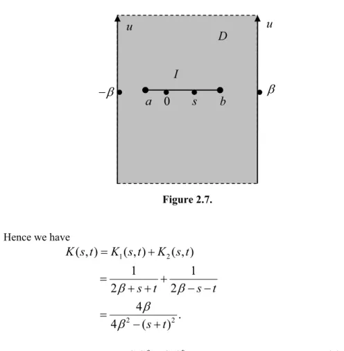
For the last part of our example we use the fact that the sum of two positive operators is positive. So if

E

!

0

and

I

[ , ]

a b

Ž

(

E E

, )

, we obtain a positive operator on

L I

₂

( )

with kernel

K s t

( , )

which is analytic in

D D

u

.

Figure 2.7. Hence we have 1 2 2 2

( , )

( , )

( , )

1

1

2

2

4

.

4

(

)

K s t

K s t

K s t

s t

s t

s t

E

E

E

E

(2.6)

Again since

K

is kernel of

S S

_{1 1}

S S

_{2 2}, (2.6) is positive definite on

L I

₂

( )

. We now give another example which is similar to the last one. This time

D

will be the horizontal strip.

a

s

b

I

D

E

u

E

u

0

Example 2.3. Let

E

!

0

and let

D

₁ be the open half-plane

^

z



£

: Im

z

E

`

. Let Ȗ be the boundary line of

D

₁ and suppose

I

[ , ]

a b

Ž

D s t

₁

, ,



I

.

We shall now construct a positive integral operator on

L I

₂

( )

whose kernel is derived from the Cauchy integral formula for functions analytic in a neighborhood of

1

D

.

Figure 2.8.

This time C.I.F. reads

1

( )

( )

2

i

f z

f s

dz

i

E

z

s

S

³

¡ .

If we put

z

i

E

u

then

dz

du

, then we get

1

(

)

( )

2

f i

u

f s

du

i

i

u

s

E

S

E

³

¡ .

This suggests the linear operator

S L

:

2

( )

¡

o

L I

2

( )

defined by

( )

( )

2

f u

du

Sf s

i

E

u

s

S

³

¡ . Hence

( )

( )

I

g t

S g u

dt

i

E

u t

³

.

0

a

s

b

1

D

I

i

E

∫

R

+i

β

f(z) ––––– dz. z – s f(iβ+ u) –––––––––– du. iβ+ u – s)

∫

R

Sf (s)

=

∫

R

(

R

)

Then we have 1 1

1

1

( , )

and ( , )

k s t

k u t

i

E

u

s

i

E

u t

. Here

k s u

₁

( , )



L I

2

(

u

¡

)

, because

2 2 ₂

1

1

I

i

E

u

s

dsdu

I

u

s

E

dsdu

³ ³

¡

³ ³

¡

Let

u

s

E

tan and

T

du

E

sec

2

T T

d

. Then,

2 / 2 2 2 / 2 2 2 2 / 2 / 2

1

sec

tan

1

(

)

.

b I a b a b a

dsdu

d ds

u

s

d ds

b a

ds

S S S S

E

T

T

E

T E

E

T

E

S

S

E

E

f

³ ³

³ ³

³ ³

³

¡ Then we have

1

1

( , )

2

1

.

(

)

(

) 2

du

K s t

i

u

s

i

u t

du

u

s i

u

i

t

E

E

S

E

E

S

³

³

¡ ¡ Figure 2.9.

¡

s i

E

t

i

E

∫

R

∫

R

K

1

(s,t) =

∫

R

=

∫

R

R (I x R), because

=

∫

R

The pole in the upper half plane is

t

i

E

. Then,

1 2 ₂

( , )

Re ( ( ),

)

2

2

.

4

K s t

i

s h u t

i

i

t

i

s i

i

t

s

i

i t

s

i

t

s

E

E

E

E

E

E

Hence 1 2 2 1

2

(

)

( , )

( , )

(

)

4

i t

s

K s t

K t s

t

s

E

E

.

Here

K s t

₁

( , )

is symmetric and positive definite.

For the second part of our example we again let

E

!

0

and let

D

₂ be the open half-plane

^

z



£

: Im

z

!

E

`

. Let Ȗ be the boundary line of

D

₂ and suppose

2

[ , ]

, ,

.

I

a b

Ž

D

s t



I

We shall now construct a positive integral operator on 2

( )

L I

whose kernel is derived from the Cauchy formula for functions analytic in a neighborhood of

D

₂.

Figure 2.10. We put

z

M

( )

u

i

E

u

and

dz

du

in C.I.F.

i

E

0

a

s

b

2

D

I

1

(

)

( )

.

2

f

i

u

f s

du

i

i

u

s

E

S

E

³

¡

This suggests the linear operator

S L

:

2

( )

¡

o

L I

2

( )

such that

( )

( )

(

)

2

f u

du

Sf s

i

E

s

u

S

³

¡ . Here 2 2

1

( , )

(

)

(

)

k s u

L I

i

E

s

u



u

¡

, because

2 2 ₂

1

1

by (2, 7).

(

)

I

i

E

s

u

dsdu

I

u

s

E

dsdu

f

³ ³

¡

³ ³

¡ Then,

2

1

( , )

(

)

(

)

2

du

K s t

i

E

s

u

i

E

t

u

S

³

¡ . Figure 2.11. The pole in the upper half plane is

s i

E

. Then,

2 2 2 2

( , )

Re ( ( ),

)

(

)

1

2

(

)

2

( , ).

4

K s t

i

s h u s i

i

i

t

i

s

i t

s

i t

s

K t s

t

s

E

E

E

E

E

E

¡

t i

E

s

i

E

f (-i

β

+ u)

–––––––––– du.

–i

β

+ u – s

∫

R

=

∫

R

(

I

x

R

), because

∫

R

=

∫

R

∫

I

1 –––––––––––––– dsdu < ∞ by (2,7) (u – s)2₊ β2

∫

R

(

R

) (

R

Here

K s t

₂

( , )

is symmetric and positive definite on

L I

₂

( )

.

For the last part of our example, we again use the fact that the sum of two positive operators is positive. So if

E

!

0

and

I

[ , ]

a b

Ž

¡

, we obtain a positive operator on

L I

₂

( )

with kernel

K s t

( , )

. Figure 2.12. 2 2 2 2 2 2

2

(

)

2

(

)

( , )

(

)

4

(

)

4

4

. (2.8)

4

(

)

i t

s

i t

s

K s t

t

s

t

s

s t

E

E

E

E

E

E

Then (2.8) is positive definite on

L I

₂

( )

. We will now consider more general half-planes.

Example 3.4. Let

0

T S

/ 2

. We define the two half planes by

^

`

^

`

1 2

:

arg

:

arg

D

z

z

D

z

z

T

T S

T S

T





£

£

1 2

[ , ],

0 so

I

a b

a

!

I

Ž

D

I

D

. Let

J

₁

w

D

₁

,

J

₂

w

D

₂ and put

Z

e

iT . We can parameterize

J

₁ by

M

( )

u

Z

,

u u



¡

.

i

E

0

a

s

b

D

I

i

E

R

(

R

.

Figure 2.13.

So C.I.F. for

D

₁ can be written as

1

( )

( )

2

f

u

f s

du

i

u

s

Z Z

S

³

¡

Z

where we do not consider

Z

and

1/ 2

S

since from Remark 1.3. and Remark 1.4. This suggests the linear operator

S

₁

:

L

2

( )

¡

o

L I

2

( )

defined by

( )

( )

2

f u

du

Sf s

u

s

S

Z

³

¡ . Then, 2 1

1

( , )

(

)

k s u

L I

u

s

Z



u

¡

,because

¡

M

0

a

T

1

D

b

I

∫

R

1

f(s)

–––––

2πi

Sf(s) =

∫

R

R

(

R

) (I x R)

2 2 2 2 2 2 2

1

1

cos

sin

1

2

cos

1

1 cos

(

)

(

)

1

.

(1 cos )

I I I I

dsdu

dsdu

u

s iu

u

s

dsdu

u

s

us

dsdu

u

s

b a

u

a

T

T

Z

T

T

T

d

d

f

³ ³

³ ³

³ ³

³ ³

³

¡ ¡ ¡ ¡ ¡ So that we have 1

1

( , )

2

(

)(

)

1

.

2

(

)(

)

du

K s t

u

s

u t

du

u

s u

t

S

Z

Z

S

Z

Z

³

³

¡ ¡ Figure 2.14

¡

t

Z

s

Z

0

∫

R

=

∫

R

∫

I

1

––––––––––––––––––

dsdu

|

u cos

θ

–s–iu sin

θ

|

=

∫

R

∫

I

≤

∫

R

∫

I

∫

R

=

∫

R

=

∫

R

R

The pole in the upper half plane is

Z

s

. Then, 1 1 2 2 2 2

( , )

Re ( ( ),

)

(

) cos

(

) sin

1

(

) sin

(

) cos

(

) sin

(

) cos

( , ).

(

) sin

(

) cos

i

K s t

i

s h u

s

s

t

i

s t

i s t

s t

i s t

s t

i s t

K t s

s t

s t

Z

Z

Z

T

T

T

T

T

T

T

T

Then we know that

K s t

₁

( , )

is symmetric and positive definite on

L I

₂

( )

.

Now we will construct our kernel for

D

₂. We can parameterize

J

₂ by

( )

u

u u

,

M

Z



¡

. Figure 2.15.

¡

M

0

I

2

D

a

b

T

R

R

.

So C.I.F. for

D

₂ can be written as

1

( )

( )

.

2

f u

f s

du

i

u

s

Z

S

Z

³

¡

This suggests us the operator

S

from

L

₂

( )

¡

to

L I

₂

( )

such that

( )

( )

2

f u

du

Sf s

u

s

Z

S

³

¡ . Hence

( )

( )

I

g t

S g u

dt

u t

Z

³

. Similarly 2 2

1

( , )

(

)

k s u

L I

u

s

Z



u

¡

. Then we have 2

1

( , )

2

(

)(

)

1

.

2

(

)(

)

du

K s t

u

s

u t

du

u

s u

t

S

Z

Z

S

Z

Z

³

³

¡ ¡ Figure 2.16.

¡

s

Z

t

Z

0

∫

R

1 f (s) = – ––––– 2πi Sf (s) =

∫

R

(

I

x

R

).

K₂(s,t) =

∫

R

=

∫

R

R (

R

)

The pole in the upper half plane is

Z

t

. Then, 2 2 2 2 2 2

( , )

Re ( ( ),

)

(

) cos

(

) sin

1

(

) sin

(

) cos

(

) sin

(

) cos

( , ).

(

) sin

(

) cos

i

K s t

i

s h u

t

t

s

i

t

s

i t

s

t

s

i t

s

t

s

i t

s

K t s

s t

s t

Z

Z

Z

T

T

T

T

T

T

T

T

Then, we know that

K s t

₂

( , )

is symmetric and positive definite on

L I

₂

( )

.

Now for the last part of the example we use the fact that the sum of two positive operators is positive. Figure 2.17.

0

a

b

I

D

T

T

BIBLIOGRAPHY

C.M.Dikmen, Positive Integral Operators with Analytic Kernels.MSc. Thesis, The University of Manchester, 1997.

N.Young. An Introduction to Hilbert space. Cambridge University Press, Cambridge, 1988. W.Rudin. Real and Complex Analysis.McGraw-Hill Book Company, New York, 1966

H.Hochstadt. Integral Equations.John Wiley & Sons Inc., New York, 1973