1-1-2017
On Detecting Faces And Classifying Facial Races
With Partial Occlusions And Pose Variations
Tarik Alafif Alafif
Wayne State University,
Follow this and additional works at:https://digitalcommons.wayne.edu/oa_theses Part of theComputer Sciences Commons
This Open Access Thesis is brought to you for free and open access by DigitalCommons@WayneState. It has been accepted for inclusion in Wayne State University Theses by an authorized administrator of DigitalCommons@WayneState.
Recommended Citation
Alafif, Tarik Alafif, "On Detecting Faces And Classifying Facial Races With Partial Occlusions And Pose Variations" (2017).Wayne State University Theses. 543.
by
TARIK ALAFIF DISSERTATION
Submitted to the Graduate School of Wayne State University,
Detroit, Michigan
in partial fulllment of the requirements for the degree of
DOCTOR OF PHILOSOPHY 2017
MAJOR: COMPUTER SCIENCE Approved By:
2017
To
my MOTHER and FATHER,
my WIFE,
my GRAND FATHER OMAR,
and my lovely kids RITAL, KHALID and the NEW COMING BABY.
We always seek his help, aid, and forgiveness.
Second, I am deeply grateful to my Ph.D. advisor, Prof. Xuewen Chen, for his continuous support and guidance throughout my Ph.D. program. Prof. Chen has taught me many things in the research eld of deep learning in computer vision. I also thank Prof. Chen for his patience and valuable feedback during my research works. This dissertation wouldn't be possible without his advices.
Third, I would like to thank all my committee members, Prof. Sreela Sasi (My Masters Degree advisor), Prof. Ming Dong, and Prof. Dongxiao Zhu for giving me constructive suggestions and comments on the dissertation. I also would like to thank Zeyad, Dr. Melih, Dr. Tin, and Dr. Thaer for their valuable comments on my research.
Fourth, I would like to give my high appreciation to my parents, my wife, and and my grand father Omar, who always support me and encourage me to pursue my Ph.D. degree.
Fifth, I would like to thank King Abdullah who passed the way a few years ago. Also, I would like to thank Saudi government represented by King Salman, Prince Mohammad Bin Naif, Prince Mohammad Bin Salman, and Saudi Arabian Cultural Mission (SACM).
Finally, I would like to give many thanks to Umm Al-Qura University, particularly to Prof. Faisal Baghdadi and Mr. Esam Alhassani for their help to send me to Wayne State University to involve in research, pursue my PhD degree, and fund me throughout my Ph.D. program.
Acknowledgements iii
LIST OF FIGURES viii
LIST OF TABLES ix
CHAPTER 1: INTRODUCTION 1
1.1 Face Detection . . . 1
1.2 Face Race Classication . . . 3
1.3 Spatial Convolution Theorem . . . 5
1.4 Deep Learning and Convolutional Neural Network . . . 6
1.5 Our Contributions . . . 9
1.6 Outline of the dissertation . . . 10
CHAPTER 2: RELATED WORK 12 2.1 Existing Labeled Face Image Datasets . . . 12
2.2 Current Face Detection Methods . . . 14
2.3 Current Facial Race Classication Methods . . . 17
2.4 Summary . . . 20
CHAPTER 3: OUR DATASETS 21 3.1 LSLF and LSLNF Datasets . . . 22
3.1.1 Automatic YouTube video links crawler . . . 23
3.1.2 Automatic YouTube video downloader . . . 23
3.1.3 Automatic frame extraction . . . 24
3.1.4 VJ face detection . . . 25
3.1.5 Automatic face and non-face image screening . . . 25 iv
3.3 Summary . . . 30
CHAPTER 4: iVJ and LSDL FACE DETECTION 31 4.1 iVJ Face Detector . . . 31
4.2 LSDL Face Detector . . . 37
4.3 Experiments . . . 44
4.3.1 Implementation . . . 44
4.3.2 Experimental Evaluations . . . 44
4.4 Summary . . . 48
CHAPTER 5: FACIAL RACE CLASSIFICATION 50 5.1 Our proposed model . . . 50
5.2 CIMN face dataset . . . 52
5.3 Experiment . . . 53 5.3.1 Implementation . . . 57 5.4 Summary . . . 59 CHAPTER 6: CONCLUSION 60 APPENDIX 62 REFERENCES 83 ABSTRACT 84 AUTOBIOGRAPHICAL STATEMENT 86 v
Figure 1.1 Example of rectangle Haar-like features. The sum of pixels which lie within the white rectangles are subtracted from the sum of pixels in the gray rectangles. Two-rectangle features are shown in (A) and (B). Figure (C) shows a three-rectangle feature, and (D) a four-rectangle feature [74]. 2 Figure 1.2 The sum of the pixels within rectangle 4 can be computed with four array
references [74]. . . 3
Figure 1.3 Challenging face examples for race classication from the CIMN dataset. 4 Figure 1.4 Spatial convolution on 2-D array [19]. . . 6
Figure 1.5 CNN architecture of LeNet-5 for digit recognition. This image is taken from LeCun [42]. . . 8
Figure 1.6 An example of partially occluded faces detected by our proposed LSDL face detector. . . 11
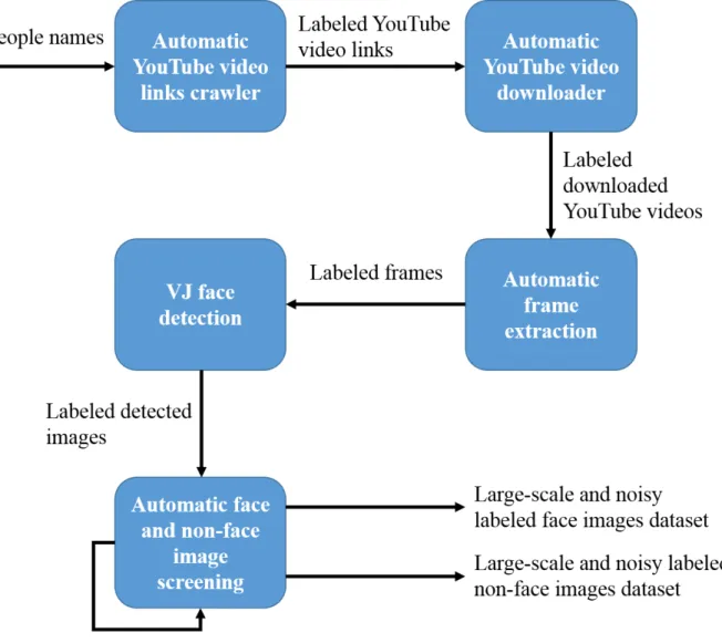
Figure 3.1 Phases for obtaining noisy LSLF and LSLNF datasets. . . 21
Figure 3.2 A sample of collected popular names for individuals. . . 22
Figure 3.3 A sample of crawled labeled YouTube video links. . . 23
Figure 3.4 A sample of labeled frames for an individual. . . 24
Figure 3.5 A sample of VJ face detection results. . . 25
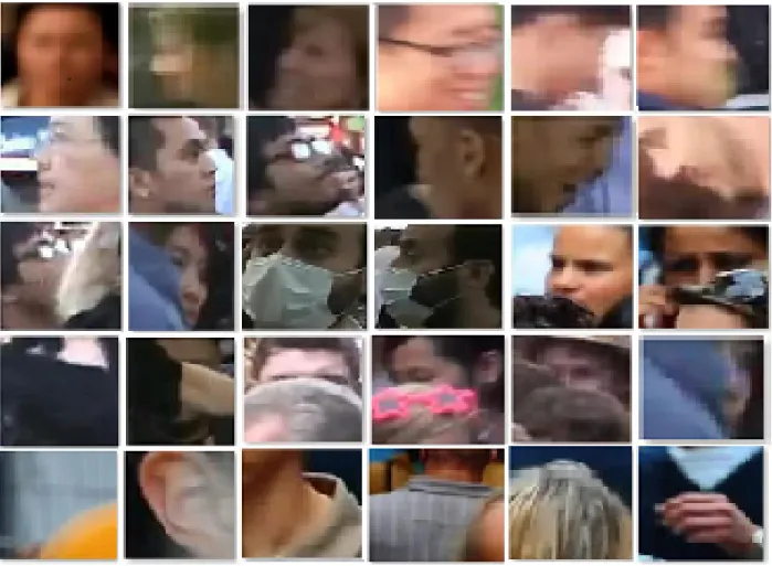
Figure 3.6 Sample images from the LSLF and LSLNF datasets. The rst three rows present face images from the LSLF dataset. Frontal and near frontal faces are presented in the rst row. Multi-view faces are presented in the second row. Partially occluded faces are presented in the third row. The last row presents non-face images from the LSLNF dataset. . . 27
view blurred faces are presented in the rst row. Multi-view non-blurred faces are presented in the second row. Multi-view light partially occluded faces are presented in the third row. Multi-view severe partially occluded faces are presented in the fourth row. The last row is a sample of
non-faces from the CrowdNonFaces dataset. . . 29
Figure 4.1 iVJ face detection pipeline. . . 31
Figure 4.2 A sample of learned kernels. . . 32
Figure 4.3 Examples of VJ and iVJ face detection results on the AFW dataset. The images in the rst column are the results of the VJ face detector while the images in the second column are the results of our iVJ face detector 33 Figure 4.4 Precision-recall curves using the AFW dataset to compare the perfor-mance between the iVJ and VJ face detectors. AP = average precision 34 Figure 4.5 The CNN model architecture for the iVJ face detector. . . 35
Figure 4.6 The CNN model architecture for the LSDL face detector. . . 40
Figure 4.7 LSDL face detection pipeline.(a) Input image. (b) Sub-windows classi-cation. (c) Condence scores thresholding. (d) NMS with the highest condence scores. (e) Final result. . . 42
Figure 4.8 Face localization map generated by the LSDL face detector. . . 42
Figure 4.9 A sample of AFW images. . . 45
Figure 4.10 A sample of FDDB images. . . 46
Figure 4.11 Precision-recall Comparisons with state-of-the-art methods using the AFW dataset. AP= average precision. . . 47
Figure 4.12 Comparisons with state-of-the-art methods using the FDDB dataset. . . 48
Figure 4.13 Qualitative face detection results by LSDL on AFW in the rst two rows and FDDB in the last two rows. . . 49
represent Caucasian faces. The images in second row represent Indian faces. The images in the third row represent Mongolian faces. The
images in bottom row represent Negroid faces. . . 51
Figure 5.3 The architecture of our CNN model. . . 52
Figure 5.4 Examples of FERET face images. . . 53
Figure 5.5 Examples of CIMN face images. . . 56
Figure 5.6 Examples of correct and incorrect race classications by our model using FERET dataset. . . 57
Figure 5.7 Examples of correct and incorrect race classications by our model and human using CIMN dataset. (a) Correct classications by our model and human. (b) Correct classications by our model but incorrect clas-sications by human. (c) Correct clasclas-sications by human but incorrect classications by our model. d) Incorrect classications by our model and human. . . 58
Figure 6.1 MTurks responses. . . 73
Table 1.1 Facial characteristics of the major four human races. . . 3 Table 3.2 A comparison of existing face datasets and our LSLF dataset. . . 28 Table 5.3 Confusion matrix for race classication in the constrained evaluation
(in %) using the FERET dataset. Abbreviations (C = Caucasian, I = Indian, M = Mongolian, N = Negroid) . . . 54 Table 5.4 Comparison against the state-of-the-art methods in the constrained
en-vironment. . . 55 Table 5.5 Confusion matrix for race classication in the unconstrained evaluation
(in %) for the proposed model and human workers on CIMN dataset. Abbreviations (C = Caucasian, I = Indian, M = Mongolian, N = Negroid) 58
CHAPTER 1: INTRODUCTION
The goal of my dissertation is to focus on 1) showing how we obtain unconstrained large-scale face datasets from the wild, 2) improving Viola-Jones (VJ) face detection results by rst training a Convolutional Neural Network (CNN) model on our noisy datasets, 3) solving face detection problems such as partial occlusions with pose variations by training a large number of faces with partial occlusions and pose variations, and 4) classifying facial races with partial occlusions and pose variations. In this chapter, we rst give a brief introduction on face detection in section 1.1. Then, we give a brief introduction on facial race classication in section 1.2. In section 1.3, we introduce and explain the convolution theorem. In section 1.4, we give a brief introduction on deep learning and Convolutional Neural Network (CNN). Then, we highlight on our contributions in this dissertation in section 1.5. Finally, we show the outlines of our dissertation in section 1.6.
1.1 Face Detection
Face detection is an important research area in computer vision since it is the rst step to be used for many computer vision related face applications. It can be used in ap-plications such as face verication, face identication, face clustering, face tracking, security access control, automatic face analysis, face image retrieval, biometrics, device and mobile communication, human computer interaction, and video surveillance. The goal of face de-tection is to determine and nd the faces in any image. However, face dede-tection is still a traditional problem in computer vision community although it has been well studied. Par-ticularly, detection problems occur when face detection methods fail to detect unconstrained partially occluded faces with dierent poses.
Many methods have been introduced in the past two decades. Thanks to the inu-ential Viola-Jones (VJ) face detector [74] that has motivated many face detection methods. The VJ method is based on rectangle Haar-like features computed by integral image and classied by a cascade of Adaboost classiers. Example of rectangle Haar-like features is shown in Figure 1.1.
Figure 1.1: Example of rectangle Haar-like features. The sum of pixels which lie within the white rectangles are subtracted from the sum of pixels in the gray rectangles. Two-rectangle features are shown in (A) and (B). Figure (C) shows a three-rectangle feature, and (D) a four-rectangle feature [74].
A rectangle 4 can be computed by the sum of the pixels with four array references [74] as shown in Figure 1.2. The value of the integral image at location 1 is the sum of the pixels in rectangle 1. The value at location 2 is the sum of the pixels in rectangles 1 + rectangle 2. The value at location 3 is the sum of the pixels in rectangles rectangle 1 + rectangle 3. Finally, the value at location 4 is the sum of the pixels in rectangles rectangle 1 + rectangle 2 + rectangle 3 + rectangle 4. Therefore, the sum within rectangle 4 can be computed as 4 + 1 - (2 + 3).
The VJ method works by rejecting false positives in early stages to detect faces. Later, Viola and Jones [34] proposed a face detection framework to handle partially rotated faces by building dierent detectors for dierent face poses. A decision tree is used to train dierent face poses to estimate the pose. However, the VJ method is computationally expensive since it requires a large number of features computations. Also, it is not an optimal face detector for unconstrained images (e.g. AFW [82] and FDDB [30]) since it results in many false positives and mostly limits detections to frontal and near frontal faces with high lightings and some extent to light partial occlusions.
Figure 1.2: The sum of the pixels within rectangle 4 can be computed with four array references [74].
1.2 Face Race Classication
Faces are the most objects that provide essential information and soft biometric traits regarding individuals such as their gender, age, expression, and race. Identifying a race from a face in an image provides a strong hint to search for facial identity and criminal identication. Some eorts in social and biological studies have been attempted to study the race using human faces as reported by Harrison et al. [24], Matt [5], and Guido [3]. They agreed on categorizing human faces into three major races, Caucasian (White), Mongolian (South east Asia), and Negroid (Black). In our work, an Indian (South Asia) race is added into our racial classication since we believe the faces from Indian race dier on many facial characteristics with other faces from other races. We provide dierent facial characteristics for the four major races in Table 1.1.
Race Skin
Cheek-bone Eyes Eyes color Nose Lips Forehead
Caucasian Light or
dark white Medium Medium Bluebrown to Medium to big Smallmedium andto thin
Medium Indian Dark white,
brown, to black
Small Medium to
big Brownblack or Small to medium Small Small Mongolian Light white,
yellow, or brown
Small to
medium Smallnarrow and Brownblack to Small to medium Small Small
Negroid Brown or
black Medium tobig Medium tobig Brownblack or Medium to big Bigthick and Big
In this work, we focus on race rather than ethnicity. The terms and the denitions of "race" and "ethnicity" are distinct although many papers in the literature do not distinguish between them. Race is dened as the physical appearance and characteristics of a person such as skin color, eye color, eye size, nose size, mouth size, cheek-bone size, facial shape, and hair type while ethnicity is referred as a culture of a person related to nationality, ritual,
Figure 1.3: Challenging face examples for race classication from the CIMN dataset. language, ideology, heritage, custom, religion, and belief [14].
A person's race is more easily identiable compared to other parts of the body. In particular, facial images belonging to a common race generally share a combination of facial feature such as skin color, bone structure, and hair texture as well as the shape of the eyes, nose and lips. This information can be extracted to reach the optimal solution for race classication.
Typically, most individuals are able to identify the race of a person if that person's face is not partially occluded or extremely rotated. A study showed that humans perform better facial race classication on their own race rather than other races [62]. Another study evaluated the performance of individuals in identifying the race for black and white races
using constrained frontal faces [23]. However, these studies were not conducted on faces with partial occlusions, extreme pose variations, low illuminations, and low resolutions. If these conditions are absent, humans may achieve 100% accuracy of race classication. Extreme changes in facial poses, facial sizes, partial occlusions, and low resolutions can cause human misclassify facial races. Challenging facial examples from CIMN dataset are shown in Figure 1. Furthermore, the race classication error rates can be varied from one person to another based on their vision accuracies especially when pose variations, low resolutions, and facial partial occlusions occur. To the best of our knowledge, no study of human performance on race classication with partially occluded, extremely rotated, and small scaled faces have been conducted. In this work, we conduct an unconstrained evaluation on human performance for race classication to study how well people perform race classication with current challenges. We compare these results with the test results of our trained model.
1.3 Spatial Convolution Theorem
In this section, we introduce the convolution theorem since it is an important part in the architecture of the CNN model. Convolution process is a linear spatial ltering technique. The convolution lter can be applied to a one dimensional array (vector) or two dimensional arrays (images). In our work, we focus on applying convolution lters to two dimensional arrays in the discrete case.
Convolution in the spatial domain is the process of moving a lter mask of two dimensional array over an image and compute the operation at each pixel location of the image [19]. A ltered image is generated when the lter moves to each pixel in the input image. One can determine the size of the convolution lter with a size of m x n where m represents the row number and n represents the column number. The convolution lter convolves on the image dened by the weights from left to right until it reaches the last position of row and column on the image.
Before performing the convolution process, the lter must be rotated to 180 degree. We pad the image with a minimum of m-1 rows of 0's and n-1 columns of 0's at the top and bottom and n-1 columns of 0's on the left and right. The lter is shifted one pixel location to the right to compute the sum of products until we reach the last position of the pixels on the image on the left. Then, we get the nal result of the convolution as shown in Figure 1.4 after cropping.
Figure 1.4: Spatial convolution on 2-D array [19]. The convolution lter computes the sum of products for each pixel as
w(x, y)Ff(x, y) =Pas=−aPbt=−bw(s, t)f(x−s, y−t) (1.1)
where w is the the convolved lter and f is the input image. x and y is the image pixel position. The minus signs on f is the rotation by 180 degree. a and b are the rows and column paddings where a = (x - 1)/2 and b = (y-1)/2. s and t are the size of the lter.
1.4 Deep Learning and Convolutional Neural Network
Deep learning has been given a large research attention to investigate the deep learning for solving many computer vision tasks including face detection. As the deep learning has
become a promising research area in computer vision, various deep learning models have been used in many classication tasks as seen in the works of [43, 28, 2]. There are several models of deep learning for supervised such as CNN for Binary and multi-task learning, and unsupervised learning such as restricted Boltzmann machines, deep autoencoder, deep belief neural network, and CNN. A model considered to be deep if it contains more than 9 layers [41]. Deep learning models allow large-scale learning by using many layers, feeding the data, and learning their feature representations. The more data in deep learning models are fed, the more invariant features are learned in which they increase the accuracy in face detection and classication. A feedforward and backpropagation are used during the feature representations learning. Another advantage of the deep learning models is that they may avoid or require less engineering works for feature extraction unlike hand-crafted features extractors such as SIFT and HOG.
The story of CNN was motivated by research of the cat's visual cortex reported by Hubel and Wiesel in the 1960's. In this work, our face detection and facial race classication models are particularly inspired by the CNN model, which was rst introduced by LeCun [42] to solve the hand digit recognition problem. Figure 1.5 shows a CNN architecture of LeNet-5 for the digit recognition problem. Generally speaking, CNN has been successfully applied to many computer vision tasks such as face detection [12, 46, 84, 16], handwritten recognition [42], face recognition [40], and image classication [38]. CNN is a hierarchical supervised multi-layer feed-forward deep learning model that works similar to biological network in human brain on receptive elds in which both contain connected neurons and many layers. The hierarchy of the CNN model consists of stack of convolution layers, sub-sampling layers, fully connected, and output layers. The input image or images start feeding the the model through the layers and neurons for training and testing. The input image or images may need a pre-processing procedure before feeding the model. Output maps (also called "feature maps") generated by one layer are the inputs for the next layer. In the convolutional layers, one or more convolved kernels are convolved on the input image
or output maps to produce output maps for the next layer. The convolved kernels are summed together and added to the bias as indicated in equation 1.1. Then, an activation non-linear function is applied to the results of the wighted sum to produce the output maps as the form of 2-D matrices. Used activation non-linear functions can be sigmoid, tanh, or Rectied Linear Unit (ReLU). The output maps include the features of the object(s) which are learned by one or more convolved kernels. The sub-sampling layers have the same number of output maps as the previous convolutional layers. It is one to one relation. In the sub-sampling layers, the outputs from the previous convolutional layers are diminished to half of their sizes for dimensional reduction by local averaging over a non-overlapping window. The averaging size is determined by a sub-sampling factor. The sum of the sub-sampling factor is multiplied by the wights and added to the bis. Then, the result is passed to the activation function to produce the output maps in the sub-sampling layer. The output maps in the sub-sampling layer improves robustness to small distortions. Then, the output maps in the sub-sampling layer are connected to one or more outputs in the next convolutional layer. The last two layers are accountable for doing the binary or multi-tasks classications using the extracted features from the previous layers. In the output layer, all the output maps from the previous layer are multiplied by the wighted sum and added the bias. Then, the results are multiplied to the activation function to perform the classication.
Figure 1.5: CNN architecture of LeNet-5 for digit recognition. This image is taken from LeCun [42].
Most of the CNN networks are trained with feedforward and backpropagation to minimize the error loss function. The model contains parameters such as weights and biases in which they are trained using supervised learning [42]. The CNN model has very high and strong discriminative capability for learning the features such as corners, edges, and shapes from object images in spatial domain. The learning for object images is performed by feeding and training object images in the form of two dimensional arrays and applying non-linear activation functions to the network. Another advantage of the CNN network, it can tolerate image distortion, illumination changes, and provide invariance of image translation. The CNN architecture shares properties of local connections, shared weights, and sub-samplings [42]. The ability of using shared weights diminishes the number of parameters in the network leading generalization. It is a powerful model for extracting and learning high level features' representations and visual variations from a large number of training image examples unlike extracting hand-crafted features using low level feature extractors such as Haar-like features [74], LBP features [72, 33, 91], NDP features [50], combined HOG-LBP features [59], and SURF [48]. Some hand-crafted feature-based methods in [26, 52, 51, 8, 18] attempted to detect partially occluded faces, but they are conned only to constrained frontal, and light partially occluded faces. An accurate face detection system must search and locate multi-view partially occluded and non-partially occluded unconstrained faces in dierent scales at dierent locations with an ecient detection speed. Usually, detecting faces in images is done by locating rectangles around the faces covering the most appeared facial features such as eyes, nose, and mouth.
1.5 Our Contributions
In this work, our main contributions are summarized as follows:
• We introduce our Large-Scale Labeled Face (LSLF) and noisy Large-Scale Labeled Non-Face (LSLNF) image datasets extracted from the wild. Furthermore, we introduce our CrowdFaces and CrowdNonFaces image datasets intended to be used for training to solve the detection problem for partial facial occlusions
• We improve VJ face detector results by rst training a CNN model on our noisy datasets. Our improvement is performed by classifying the VJ detected results and eliminating false positives. We show our improvement over the VJ face detector on AFW face detection benchmark dataset.
• We propose a Large-Scale Deep Learning (dubbed as LSDL), a face detection method that does not require training several CNN models for facial parts, hand-crafted fea-tures computation, or both to localize facial parts and faces. Our LSDL method uses a single trained CNN model to detect unconstrained multi-view partially occluded and non-partially occluded faces. The model is trained with non-noisy training examples from our four datasets and Annotated Facial Landmarks in the Wild (AFLW) dataset. Our LSDL method is evaluated on two popular face detection benchmark datasets, Annotated Faces in the Wild (AFW) and Face Detection Dataset and Benchmark (FDDB). An example of face detection by our detector is depicted in Figure 1.6. • We propose a CNN model to classify facial races with partial occlusions and pose
variations. The proposed model is trained with unconstrained multi-view partially occluded and non-partially occluded faces using a broad and balanced racial distributed face dataset. The model is trained on four human races: Caucasian, Indian, Mongolian, and Negroid. Our model is evaluated against state-of-the-art methods on constrained face test datasets. Also, an unconstrained evaluation of the proposed model and human performance is conducted and compared using our new benchmark face test dataset.
1.6 Outline of the dissertation
The remainder of this dissertation is organized as follows. In Chapter 2, we review existing labeled face image datasets. We also review the related work on face detection and facial race classication. In Chapter 3, we introduce the collection mechanism for obtaining our image datasets. In Chapter 4, we present our two proposed methods for face detection, the improved Viola-Jone (iVJ) and Large Scale Deep Learning (LSDL) methods. A perfor-mance comparison for the iVJ and VJ is provided using the AFW face detection benchmark
Figure 1.6: An example of partially occluded faces detected by our proposed LSDL face detector.
dataset. An experimental implementation and evaluation of the LSDL method are provided. Our LSDL method is evaluated on two common face detection benchmark datasets, the AFW and FDDB, against the currently published methods. In Chapter 5, we present our CNN model to classify facial races with partial occlusions, pose variations, and low resolutions. The architecture and training of the proposed CNN model are introduced. A new facial race benchmark dataset is introduced. We present our experimental evaluations in the con-strained and unconcon-strained environments. In the concon-strained environment, we evaluate our model against state-of-the-art works using FERET constrained frontal face images. In the unconstrained environment, we present the evaluation of our model and human performance using our CIMN dataset. Implementation details are also provided. Finally, we conclude our work in Chapter 6.
CHAPTER 2: RELATED WORK
In this chapter, we rst provide some details on the existing labeled face image datasets in section 2.1. Second, we overview the most recent and old face detection methods and highlight on their strengths and weaknesses in section 2.2. Third, we review the related works on facial race classication in section 2.3.
2.1 Existing Labeled Face Image Datasets
Many existing labeled face datasets have been available for dierent goals, but they tend to be in small-scales in both constrained and unconstrained environments. These datasets are briey overviewed as follows:
Labeled Faces in the Wild (LFW) Dataset [29]. The LFW is a face verica-tion benchmark dataset. It consists of 13,749 unconstrained labeled face images for 5,749 individuals. The size of the images are 250 x 250 in JPEG extensions. The images were automatically labeled. This dataset was collected from web news articles. The face images in LFW dataset have variations in color and grayscale, near frontal poses, lightings, reso-lutions, quality, age, gender, unbalanced race, accessory, partial occlusions, make up, and background. The dataset size is 179 MB. The LFW face dataset intended to be made for face verication problem, which they call it the pair matching problem. It is publicly available for downloading.
WebV-Cele Dataset [9]. The WebV-Cele is a large-scale dataset in which it consists of 649,001 face images for 2,427 celebrities. Only 42,118 face images are manually labeled. The face images were collected from YouTube videos. The images have variations in color and grayscale, quality, resolution, pose, illumination, background, human face, facial expression, partial occlusion, make up, gender, race, accessory, tattoo, hat, glasses, sunglass, hand, scarves, and microphone. The dataset is available upon request.
CAS-PEAL Dataset [15]. The CAS-PEAL is a large-scale dataset in which it consists of 99,594 manually labeled face images for 1,040 individuals, 595 males and 445
females. The dataset is designed for face recognition. The face images were captured in a studio in constrained environment with nine cameras from dierent angles at dierent times. The images have many variations in color and grayscale , expression, lighting, pose, background, and accessory such as hat and glasses. The disadvantage of CAS-PEAL dataset is that it only contains Chinese faces. The dataset size is nearly 26.6 GB. Only part of this dataset is publicly available. Other part is obtained upon request.
Face Recognition Grand Challenge (FRGC) Dataset [61]. The FRGC dataset contains of nearly 50,000 manually labeled face images including 3D scans and images for 466 individuals. The face images were collected from a studio in constrained environment. The images have variations in color, lighting, expression, background, race, 3D scan, and image sequence. The dataset size is 3.1 MB. The dataset is available upon request.
Multi-PIE Dataset [20]. The Multi-PIE dataset consists of 755,370 manually la-beled face images. It consists of very small number of individuals (337 individuals). Most of the individuals are men. The face images were captured in a studio in constrained envi-ronment from 15 view points and 19 illumination conditions. The images have variations in color, resolution, pose, illumination, and expression. The size of the images are 3072 x 2072. The dataset size is 400 GB. The dataset is commercial.
FERET Dataset [63]. The FERET dataset consists of 14,126 manually labeled face images for 1,199 individuals. The face images were captured in a studio in constrained environment. The images have variations in color, pose, and illumination. The dataset is available upon request. The dataset is intentionally designed for face recognition.
Extended Yale B Dataset [17]. The Extended Yale B dataset consists of 16,128 face images for 28 individuals. The dataset is intentionally designed for face recognition. The face images were collected from a studio in constrained environment. The images have variations in grayscale, pose, and illumination. The dataset is available upon request.
2.2 Current Face Detection Methods
Many face detection methods have been proposed in the past decades. Face detection method using skin color was popular and proposed by Hsu et al. [27]. This method, however, was sensitive to lighting changes. An old face detection survey has been done in [89] and modied recently in [86]. Although the eld has advanced considerably, some challenges still remain under unconstrained environments. In particular, detecting faces under partial occlusions with pose variations remains a challenge that has not been well addressed by current methods.
Most current face detection methods have been generally inuenced by the idea of cascading, Deformable Parts Model (DPM), Neural Network (NN), and CNN-based methods. Current face detection methods can be briey overviewed in four dierent groups as follows: • NN-based methods: Several methods have been proposed in [73, 65, 71, 13, 66] which apply NNs to detect faces in multiple scales at all possible locations. Vaillant et al. [73] rst trained a simple NN with 2-hidden layers to detect the presence and absence of a frontal face at dierent scales in an image. Rowley et al. [65] proposed another simple NN-based method with three types of hidden units in one layer to detect upright and frontal faces in constrained gray-scale images. Each type of hidden units is dedicated for detecting particular features in the face. Followed by the works of Vaillant et al. [73] and Rowley et al. [65], Sung and Poggio [71] used a multilayer perceptron NN to detect frontal faces. Later, Feraund et al. [13] presented a combined Constrained Generative Models (CGMs) on top of a multilayer perceptron NN to compute the probability of having a face in a tested grayscale image. Then, Rowley et al. [66] used two NNs consisting of 1-hidden layer each to detect partially in-plane, upright, and frontal rotated faces. However, existing NN-based methods are not able to handle the detection of extreme facial rotations and partial facial occlusions.
• Cascade-based methods: These methods follow the cascading idea of the VJ face detector such as FloatBoost [49], MVFD-cascade [77], Soft-cascade [4], SURF-cascade
[48], HeadHunter [57], ACF [83], Joint-cascade [7], and NPD-cascade [50]. Li and Zhang [49] rst proposed a FloatBoost learning algorithm with a statistical model to detect multi-view faces using a detector-pyramid. Then, Wu at al. [77] used a condence-rated look-up-table with Real Adaboost cascade classiers to estimate face poses. Bourdev and Brandt [4] proposed a face detector based on a soft cascade clas-sier to detect frontal upright faces. Li and Zhang [48] used multi-dimensional SURF features with a Gentle Adaboost cascade classier instead to improve the speed of the VJ face detector training. Mathias et al. [57] adapted ve dierent squared integral channel features to the task of unconstrained frontal and rotated face detection. Yang at al. [83] applied a soft cascade classier to aggregated channel features for improving multi-view face detection. Later, Chen et al. [7] used pixel dierences as a feature and aligned faces for face detection with Real Adaboost cascade classiers. Recently, Liao et al. [50] presented a face detector using a combination of simple Normalized Pixels Dierence (NPD) features and deep quadratic tree classiers to learn faces. A single soft-cascade classier is used for face detection. In general, the performance of cascade-based face detection methods are computationally intensive since they require computing a large number of hand-crafted features for trained cascade detectors. • DPM-based methods: These types of methods use a collection of deformable facial
parts models and HOG features for face detection. These methods depend on human body and facial landmarks annotations or facial landmarks bounding boxes for train-ing. Examples of these methods include TSM [92], DPM-cascade [81], DPM-cascade Pruning [80], Structural Face Model [82], and Vanilla-DPM [57]. Zhu and Ramanan [92] used a mixture of trees with a shared pool of parts to detect faces, estimate their poses, and localize their landmarks. However, this method requires manual facial land-mark and pose annotations to model the facial parts before training. Followed by the work of Zhu and Ramanan [92], Yan et al. proposed part-based cascade methods to improve the speed for face detection reported in [81] and [80]. These methods require
bounding box annotations instead of facial landmarks annotations introduced by Zhu and Ramanan [92] for training the detection systems. Yan et al. [82] also presented a tree-based structural model trained on an SVM for face detection. This method attempted to explore the face-body co-occurrence to improve the detection under oc-clusion. Later, Mathias et al. [57] used DPM with HOG low level features trained on an SVM classier for multi-view face detection. However, these types of methods require training annotated body and facial landmarks in order to locate the faces. This is not suitable for detecting partially occluded faces in real world scenes since human bodies may have many dierent articulations and may be hidden or occluded. Although DPM-based methods train faster than cascade-based methods with fewer training examples, they are still computationally intensive since they require HOG low level features computations.
• CNN-based methods: Compared to NN-based methods that use shallow NNs which tend to overt for large-scale learning, CNN-based methods employ a deeper architec-ture than NNs in terms of the number of layers and nodes to get more robust high level feature representations learning. A few of face detection methods such as CFF [16], Cascade CNN [46], MTL [90], DDFD [12], and Faceness-Net [84] presented dierent CNNs models for face detection. First, Garcia and Delakis [16] presented two convo-lutional layers in a CNN binary classier focusing on detecting only partially rotated faces at dierent scales. The detection was done by projecting face candidates to their original scales. Li et al. [46] followed the idea introduced by Viola and Jones [74] and applied a cascade of CNNs to detect rotated faces by eliminating non-face candidates in early stages. This in turn helps to reduce the number of candidates left for later stages. Then, Zhang and Zhang [90] introduced three convoluional layers in a multi-task deep CNN model trained on partially rotated constrained faces to learn faces, estimate their poses, and localize their landmarks. Similar to the work of Zhang and Zhang [90], Farfade et al. [12] proposed a Deep Dense Face Detector (DDFD) to detect multi-view
unconstrained faces with more condence on up-right faces using a single CNN model. However, current methods are presented by Li et al. [46], Zhang and Zhang[90], and Farfade et al. [12] still fail to detect partially occluded faces. The failure is due in part to lack of partially occluded face training examples in AFLW dataset. Recently, Yang et al. [84] proposed a face detection method called Faceness-Net to handle the detection of partially occluded faces by detecting ve facial landmarks' (e.g. hair, eyes, nose, mouth, and beard) responses. The responses were generated after training sev-eral and dierent independent CNN models for each part to generate their partness maps. The maps were combined together and computed using spatial congurations to locate the faces. However, the Faceness-Net method is computationally intensive since it requires training several independent CNN models for facial landmarks and also requires hand-crafted features computation to localize facial parts and faces.
Previous methods are not capable of handling the detection of partially occluded faces except the works are presented by Liao et al. [50], Li et al. [46] and Yang et al. [84]. Compared to these methods, our proposed LSDL face detection method does not require training several CNN models or hand-crafted features computations to locate the faces. Our method uses only a single CNN model. Our work is motivated by Farfade et al. [12] where similar depth for the CNN model is used for more robust feature representation learning. Our CNN model, however, is trained on our large-scale data to handle the detection problem of multi-view partially occluded faces.
2.3 Current Facial Race Classication Methods
Race classication has become an important research topic recently since it provides strong hint for face recognition and criminal identication. A number of recent surveys for iris and facial based race classication have been reported in [14] [70] [55] [11]. Many works have been studied on how the race feature can be classied from human faces.
Several race classication methods use facial images for race classication. In early race classication works, Wechsler and Philips [22] rst attempted to use hybrid classication
architectures of ensemble of radial basis functions (RBF) networks and inductive decision trees (DT). Their method was measured on FERET face database and achieved an over-all 94% accuracy of race classication task on four races, Caucasian, Asian, Oriental, and African. Hosoi et al. [25] introduced a method based on Gabor Wavelet Transformation and Retina sampling to extract Gabor features from face images. Support Vector Machine (SVM) classier was used. Their method was tested on MBGC and Mogshots datasets. They achieved an accuracy of 97%, 97%, and 95% on MBGC dataset and 98% 95%, and 96% on Mogshots dataset for classifying Mongolian, Caucasian, and Negroid races respectively. Race classication was also addressed using a Linear Discriminant Analysis (LDA) scheme [53] to classify Asian and non-Asian faces. They achieved 92% accuracy of race classication. A combination of 263 face images from Yale, AR, AsianPF01, NLPR constrained databases were used for the testing their method. Kumar et al. [39] used race and 65 other describable visual attribute from facial images to train an SVM for face verication. Then, Yang and Ai [85] used a Local Binary Pattern Histogram (LBPH) with an AdaBoost classier for classify-ing Asian and non-Asian faces. They evaluated their method with three face image datasets, FERET, PIE, and snapshot acquired in constrained and achieved 93.2% of race classica-tion accuracy. Instead of using hand-crafted feature extractors, Ahmed et al. [1] presented a framework for training CNN model using transfer learning from pseudo tasks for facial race classication. Three classes of races were used, White, Asian, and other for the their exper-iment. Their method achieved 93.9% accuracy of ethnicity classication using FRGC v2.0 database. Guo and Mu [21] used biologically-inspired features (BIFs) with manifold learning and an SVM to estimate races as Black, White, Hispanic, Asian, and Indian from facial faces using MORPH-II database. They achieved 98.3%, 97.1%, 74.2%, 59.5%, and 6.9% of estimation accuracy respectively to the corresponding classes. An overall of 67.2% accuracy of ethnicity estimation on all classes is achieved. Han et al. [23] also used BIFs to extract racial feature from faces and applied hierarchical classier to classify Black and White races. Xie at al [79] applied a Kernel Class-dependent Feature Analysis (KCFA) combined with
facial color based features. Their method was tested for Caucasian, African, and Asian races using MBGC and Mogshots datasets. They achieved a classication accuracy of 97%, 97%, and 95% using MBGC dataset and 98% 95%, and 96% on Mogshots dataset respectively for the corresponding races. Chen and Ross [6] proposed a Local Gradient Gabor Pattern (LGGP) method to classify Asian, Caucasian, and African race from faces. Recently, Wang et al. [75] proposed a CNN model for constrained frontal facial race classication. They evaluated their model on black vs. white and Chinese vs. Non-Chinese. They achieved classication accuracy rates of 100%, 99.4%, 99.8%, and 99.9% respectively for each race. The black vs. white classication was tested on MORPH II face image dataset. The Chinese vs. Non-Chinese classication was tested on a large collection of face images from IDPhotos, CAS-PEAL, CASIA-WebFace, Multi-PIE and MORPH II face datasets.
Instead of using facial images, some other methods used iris and periocular region images for race classication. Qiu et al. [64] used a bank of 2D Gabor lters with an AdaBoost classier to classify Asian and non-Asian iris images. Later, Qiu et al. [78] con-tinued their research and used Gabor lters and k-means for clustering iris images. Features were extracted from iris images and clustered to Asian and on-Asian race categories. Then, SVM was applied to feature vectors for nal classication. They used 2,400 iris samples and achieved an overall 91.02% of classication accuracy. The experiment was measured on CASIA-BioSecure iris database. Lyle at al. [54] applied a Local Binary Pattern (LBP) with an SVM to classify Asian and non-Asian periocular region images. Recently, Zarei and Mou [88] used articial neural networks for iris race classication. Their method was measured using University of Notre Dame's iris database. An overall of 93.3% classication accuracy was achieved on Asian and Caucasian classes. However, iris and periocular region based race classication methods are only conned to constrained frontal faces. These methods are most likely to fail when eyes are partially occluded or faces are extremely rotated.
From our literature review, two problems need to be addressed. First, existing facial race classication methods are only conned to constrained non-partially occluded frontal
faces. Therefore, we present in this dissertation a trained CNN model that is able to classify facial races with partial occlusions and pose variations under unconstrained environments. Our model is similar to the model presented by Wang et al. [75], but trained with un-constrained multi-view partially occluded and non-partially occluded faces to handle the classication of facial races with pose variations and partial occlusions. Second, there are no common benchmark datasets for evaluating the facial race classication methods. The current methods are only evaluated on frontal faces using dierent race test datasets. More-worse, many of these test datasets are private and are not available. In addition to the lack of common race benchmark datasets, the current methods use dierent racial classes for their evaluations. To address this issue, we introduce our facial race benchmark (CIMN) dataset which includes annotated multi-view and partially occluded faces for Caucasian, Indian, Mongolian, and Negroid races.
2.4 Summary
In this chapter, we reviewed in details the existing labeled face image datasets. Also, we reviewed in details the current face detection and race classication methods. While reviewing, we highlighted the strengths and weaknesses of these methods. In chapter 3, we will introduce our datasets and show how we obtain them from the wild.
CHAPTER 3: OUR DATASETS
In this chapter, we describe the methodology for obtaining our Large Scale Labeled Face (LSLF) dataset, noisy Large Scale Labeled Non-Face (LSLNF) dataset in section 3.1. Then, we provide the details for obtaining CrowdFaces dataset, and CrowdNonFaces dataset in section 3.2. We show in this chapter how these datasets are extracted from the wild. These datasets are very essential since they provide a large number of unconstrained facial and non-facial image variations for training. The datasets are briey explained as follows:
3.1 LSLF and LSLNF Datasets
We rst used Wikipedia and other online resources to collect 11,690 popular names for individuals from many countries all over the world. Figure 3.2 shows a sample of collected popular names for individuals. The individual names include celebrities in many categories such as politics, sports, journalism, movies, arts, and educations. Most individuals' names consist in our datasets are associated with the individual's rst name then last name or vice versa while the rest of the names are famous nick names or popular single names. There is no matter for ordering the individual's rst name and last name.
Figure 3.2: A sample of collected popular names for individuals.
We employ a systematic procedure consisting of ve phases to obtain noisy LSLF and LSLNF image datasets as shown in Figure 3.1. The ve phases consist of automatic YouTube video links crawler, automatic YouTube video downloader, automatic framing extraction, VJ
face detection, and automatic face and non-face screening. The phases are briey explained as follows:
3.1.1 Automatic YouTube video links crawler
In this phase, we developed a YouTube video links crawler to read the collected indi-vidual names and automatically retrieve and collect YouTube video links for each indiindi-vidual. The individualsâ YouTube video links still can be retrieved even If the ordering of the names is dierent. The links are associated and written for each labeled individual name in a text le. A sample of crawled labeled YouTube video links is shown in Figure 3.3.
Figure 3.3: A sample of crawled labeled YouTube video links.
3.1.2 Automatic YouTube video downloader
After retrieving YouTube video links using our automatic video links crawler, we developed a YouTube video downloader to automatically download the YouTube video links
belonging to each individual. The labeled videos were stored to corresponding individual's labeled name. The total number of downloaded labeled videos is 129,435 videos with a total size of 2.96 TB. All the labeled videos were stored in mp4 format for 11,690 individuals where individuals have a minimum of 1 video and a maximum of 68 videos. Our labeled YouTube video dataset has a larger number of labeled videos per person and a larger number of people among other existing labeled video datasets such as YouTube Faces [76] and WebV-Cele [9].
3.1.3 Automatic frame extraction
After downloading the labeled YouTube videos, we automatically selected and ex-tracted a number of frames per video. The frame selection per video was based on rounding to the nearest integer from the number of frames divided by forty to obtain frames that include dierent facial poses and partial occlusions. Following this procedure, we obtained 5,033,177 frames with a total size of 178 GB. All the frames were stored in JPEG format and labeled for 11,690 individuals where individuals have a minimum of 34 frames and a maximum of 2,716 frames. The dierence of frames number for each individual is due to the dierent number and the length of downloaded videos. The average number of frames per individual is 430. A sample of labeled frames for an individual is shown in Figure 3.4.
3.1.4 VJ face detection
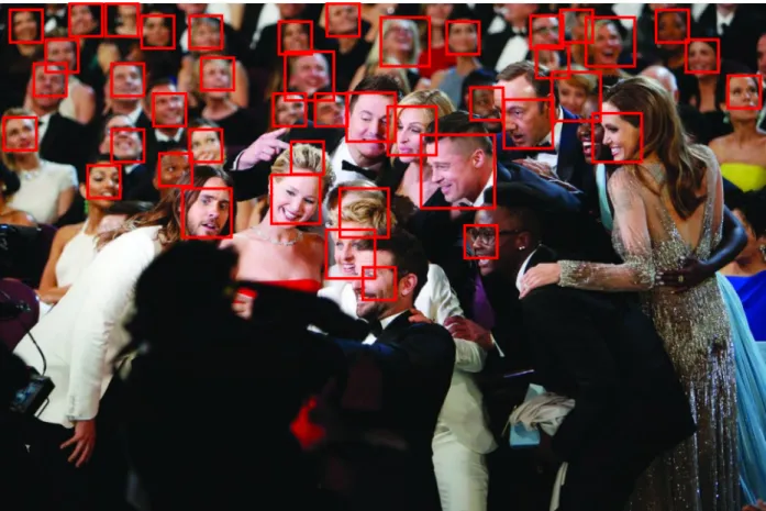
After extracting and storing the labeled frames, we automatically applied the VJ face detector to all labeled frames to detect faces. By applying VJ face detection, many face and non-face examples were detected due to a drawback of the VJ face detector that results in many false positives. Each detected example was automatically labeled and associated with the same name as used for the individuals. The number of labeled images is 9,750,456 with a total size of 38.8 GB. All the images were stored in JPEG format for 11,690 individuals where individuals have a minimum of 3 images and a maximum of 6,697 images. The dierence of labeled images number for each individual is due to the dierent number of labeled frames and the dierent number of detected faces in each frame. The average number of detected images per individual is 834. A sample of VJ face detection results is shown in Figure 3.5.
Figure 3.5: A sample of VJ face detection results.
3.1.5 Automatic face and non-face image screening
In this phase, we automatically separated out face and non-face examples as much as possible from the results of the VJ face detection using several automatic screenings. For automatic image screenings, several trained classication models such as Frontal Face (LBP),
Eye Pair, Single Eye, Single Eye (CART), Prole Face, Mouth, and Nose were applied to the results of the VJ face detection phase.
After completing this screening phase, we obtained the LSLF and LSLNF datasets with slight noise. Here, the noise referred to is the false positives resulted after classication. To be specic, LSLF contains about 1.7% non-faces while LSLNF contains about 10% faces. After completing the screening phase, individuals with 0 images are automatically removed from both datasets. Therefore, our noisy LSLF dataset consists of 1,217,185 labeled face images for 11,478 individuals with about 1.7% noise. These face images are stored in JPEG format with a size of 5.49 GB. Individuals have a minimum of 1 face image and a maximum of 1,177 face images. The average number of face images per individual is 106. On the other hand, our noisy LSLNF dataset consists of 3,468,430 labeled none-face images for 11,682 individuals with about 10% noise. These non-face images are stored in JPEG format with a size of 13.2 GB. Individuals have a minimum of 1 non-face image and a maximum of 2,282 non-face images. The average number of non-face images per individual is 296.
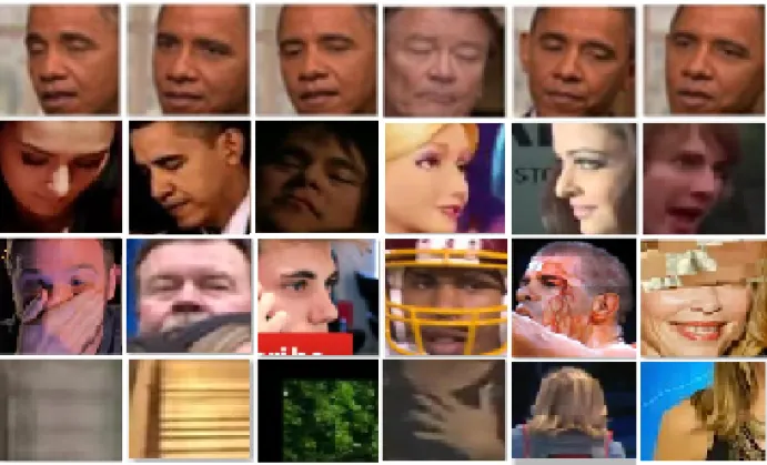
After obtaining the noisy LSLF dataset, we manually removed the noise from it. Therefore, our LSLF dataset consists of 1,195,976 labeled face images for 11,459 individuals. These face images are stored in JPEG format with a size of 5.36 GB. Individuals have a minimum of 1 face image and a maximum of 1,157 face images. The average number of face images per individual is 104. Each image is automatically labeled as "Name of person_Video number_Frame number_Detected Image number". Image samples from the LSLF and noisy LSLNF datasets are shown in Figure 3.6.
Our LSLF dataset consists of multi-view faces. Many of these faces have frontal and near frontal poses. These faces have large image variations in color and grayscale, image quality, image resolution, image illumination, image background, image illusion, human face, cartoon face, facial expression, light and severe partial facial occlusion, make up, gender, age, and race. Also, our LSLF dataset has a broad distribution of races from dierent parts of the world. Many of our face images are partially occluded with accessories such as tattoos,
Figure 3.6: Sample images from the LSLF and LSLNF datasets. The rst three rows present face images from the LSLF dataset. Frontal and near frontal faces are presented in the rst row. Multi-view faces are presented in the second row. Partially occluded faces are presented in the third row. The last row presents non-face images from the LSLNF dataset.
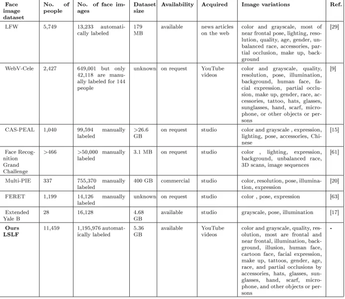
hats, glasses, sunglasses, hands, hair, beards, scarves, microphones, or other objects or persons. These factors essentially make our dataset great for large scale face learning and face recognition tasks. To the best of our knowledge, our LSLF dataset is the largest labeled face image dataset in the literature in terms of the number of labeled images and the number of individuals compared to other existing face image datasets [29, 9, 15, 61, 20, 63, 17]. A brief comparison is made in Table 3.2.
3.2 CrowdFaces And CrowdNonFaces Datasets
We introduce our two other datasets extracted from the wild, CrowdFaces and Crowd-NonFaces datasets. The objective of these datasets is to obtain multi-view blurred and non-blurred faces, multi-view partially occluded faces, and non-faces to be used for the training. For obtaining these datasets, we manually selected and downloaded thirty YouTube videos
Face image dataset
No. of
people No. of face im-ages Datasetsize Availability Acquired Image variations Ref. LFW 5,749 13,233
automati-cally labeled 179MB available news articleson the web color and grayscale, most ofnear frontal pose, lighting, reso-lution, quality, age, gender, un-balanced race, accessories, par-tial occlusion, make up, back-ground
[29]
WebV-Cele 2,427 649,001 but only 42,118 are manu-ally labeled for 144 people
unknown on request YouTube
videos color and grayscale, quality,resolution, pose, illumination, background, human face, fa-cial expression, partial occlu-sion, make up, gender, race, ac-cessories, tattoo, hats, glasses, sunglasses, hand, scarf, micro-phone, or other objects or per-sons
[9]
CAS-PEAL 1,040 99,594 manually
labeled >GB26.6 on request studio color and grayscale , expression,lighting, pose, accessories, Chi-nese [15] Face Recog-nition Grand Challenge >466 >50,000 manually
labeled 3.1 MB on request studio color , lighting, expression,background, unbalanced race, 3D scans, image sequences
[61]
Multi-PIE 337 755,370 manually
labeled 400 GB commercial studio color, resolution, pose, illumina-tion, expression [20] FERET 1,199 14,126 manually
labeled unknown on request studio color , pose, expression [63] Extended
Yale B 28 16,128 4.68GB available studio grayscale, pose, illumination [17] Ours
LSLF 11,459 1,195,976 automat-ically labeled 5.36GB available YouTubevideos color and grayscale, quality, res-olution, most are frontal and near frontal, illumination, back-ground, illusion, human face, cartoon face, facial expression, make up, tattoos, gender, age, race, and partial occlusions by accessories, hats, glasses, sun-glasses, hand, scarf, micro-phone, and other objects or per-sons
-Table 3.2: A comparison of existing face datasets and our LSLF dataset.
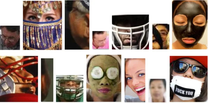
that include crowd scenes in streets, sport games, religious gatherings, parties, street ghts, and courts. Partially occluded faces are occluded by overlapping objects such as faces, hands, bodies, hats, masks, hair, etc. An overlapping sliding window is applied to these scenes at all locations with dierent scales to extract non-faces, multi-view blurred and non-blurred faces, and multi-view partially occluded faces. The sliding window starts at size 16 x 16 and increases by 1.5 scaling factor until the window size is no larger than the frame. We manually curated 10,049 faces and 31,662 non-faces at dierent scales from these sub-windows. Our partially occluded face images include light and severe partially occluded faces. A sample of these images is shown in Figure 3.7.
Figure 3.7: Sample images from the CrowdFaces and CrowdNonFaces datasets. The rst four rows are a sample of faces from the CrowdFaces dataset. Multi-view blurred faces are presented in the rst row. Multi-view non-blurred faces are presented in the second row. Multi-view light partially occluded faces are presented in the third row. Multi-view severe partially occluded faces are presented in the fourth row. The last row is a sample of non-faces from the CrowdNonFaces dataset.
3.2.1 Implementation
We implemented the rst three phases for obtaining LSLF and LSLNF datasets in PHP while the remaining phases were implemented in Matlab 2015b. These datasets were acquired and screened within a span of nearly 18 months. Our datasets are now pub-licly available at http://discovery.cs.wayne.edu/lab_website/index.php/lsdl/ for re-search and non-commercial use only.
3.3 Summary
In this chapter, we introduced our four face image datasets, LSLF, noisy LSLNF, CrowedFaces, and CrowedNonFaces datasets. We showed how we obtained these datasets from the wild. These datasets are tremendously benecial for large scale face and non-face learning since they contain a large number of non-face images and face images with partial occlusions and pose variations. In chapter 4 and 5, we show how we can take the advantages of these datasets and use them for training our face detection and facial race classication models.
CHAPTER 4: iVJ and LSDL FACE DETECTION
In this chapter, we present our two proposed face detection methods. The rst method focuses on improving the VJ face detection results which we call it iVJ. The iVJ face detector will be explained in details in section 4.1. In the second method, a Large-Scale Deep Learning (LSDL) face detection method is presented in details in section 4.2. Then, we provide the training, implementation, and evaluation details for both methods.
4.1 iVJ Face Detector
This section introduces our rst proposed face detection method, iVJ. The objective of our iVJ method is to improve the results of the VJ face detector since it results in many false positives. The iVJ face detection pipeline is shown in Figure 4.1. The key ideas are to 1) use a powerful single CNN model for feature extraction and classication to classify the results of the VJ face detection and 2) eliminate false positives resulting from the VJ face detection. Our iVJ method uses a single trained CNN model to classify the detected images
Figure 4.1: iVJ face detection pipeline.
resulted from the VJ face detector. Our model is trained with 160K noisy face and non-face examples. The noisy face and non-face examples were collected from our LSLF and LSLNF datasets. We collected 80K noisy face examples and 80K noisy non-face examples, resized them to 100 x 100, and then normalized them for training our model. For training, we used 0.1 learning rate. Our trained CNN model architecture consists of eight layers, excepting the input image (retina). The model receives the input image with a dierent resolution
resulted from the VJ face detector which our model classies it to be a face or a non-face. The architecture puts in practice the concept of receptive eld and weight sharing. It consists of three convolutional layers, three sub-sampling layers, one fully-connected layer, and one output layer. A sigmoid nonlinear activation function is applied to the model's inputs to learn the representation and transformation of data through the layers and computed as
Sigmoid(x) = 1/(1 +e(−x)) (4.1)
Kernel weights are randomly initialized. Biases are initialized to zero. The kernels are learned during convolution in the convolutional layers to learn automatically the edges and corners of the training examples by the weights of respective feature maps. In our method, we used 5 x 5, 5 x 5, and 3 x 3 trainable kernels sizes respectively for the convolutional layers. A sample of the learned kernels during the training is shown in Figure 4.2.
Figure 4.2: A sample of learned kernels.
Each feature map corresponding to a convolution with a learned kernel is learned by the weights which are a combination set of facial features. The feature maps during the convolutions are computed as
f m(cl)=φ(l)Xw(l)(u, v)y(l−1)(x+u, y+v) +b(l) (4.2)
wheref mc is the weighted sum multiplied by the sigmoid nonlinear activation functionφ. x and y are the feature map size whileuand v are the kernel K size. l is the current layer. w
Figure 4.3: Examples of VJ and iVJ face detection results on the AFW dataset. The images in the rst column are the results of the VJ face detector while the images in the second column are the results of our iVJ face detector
to perform local averaging and sub-sampling to reduce the size of the feature maps. From Figure 4.6, we have 6 feature maps with size 48 x 48 in the rst sub-sampling layer. In the
Figure 4.4: Precision-recall curves using the AFW dataset to compare the performance between the iVJ and VJ face detectors. AP = average precision
second sub-sampling layer, we have 12 feature maps with size 22 x 22. We have 24 feature maps with size 10 x 10 in the third sub-sampling layer. In the last sub-sampling layer, we have 48 feature maps with size 4 x 4. The feature maps during the sub-sampling layers are computed as
f m(sl)=φ(l)(w(l)Xy(l−1)(2x+u,2y+v) +b(l)) (4.3)
where f ms is the sum of sub-sampled feature maps multiplied by the weight w and the sigmoid nonlinear activation function φ. One can notice the number of feature maps are
Figure 4.5: The CNN model architecture for the iVJ face detector.
The last two fully-connected layers are accountable for doing the binary classication task using the extracted features from the previous layers. The last output neuron is a binary classier which returns the value 1 if the detected image is a face and value 0 otherwise.
From Figure 4.5, we have 6 feature maps with size 96 x 96 in the rst convolutional layer. Each feature map unit computes the weighted sum of its input by 25 (5 x 5) trainable coecients and add a trainable bias. Therefor, the rst convolutional layer has 156(6 x 26) trainable parameters. In the rst sub-sampling layer, we have 6 feature maps of size 48 x 48 corresponding to each feature map in the rst convolutional layer. The receptive eld for each unit is with the size 2 x 2 from the feature maps in the previous layer. Each sub-sampled feature map is reduced to half the size of feature maps from the previous layer. Therefore, the rst sub-sampling layer has 12 (6 x 2) trainable parameters. In the second convolutional layer, we have 12 feature maps with size 44 x 44. The same as in the rst convolutional
layer, each feature map unit computes the weighted sum of its input by 25 (5 x 5) trainable coecients and a trainable bias. Therefore, the second convolutional layer has 312 (12 x 26) trainable parameters. In the second sub-sampling layer, we have 12 feature maps of size 22 x 22 corresponding to each feature map in the second convolutional layer. The receptive eld for each unit is with the size 2 x 2 from the feature maps in the previous layer. Each sub-sampled feature map is reduced to half the size of feature maps from the previous layer. Therefore, the second sub-sampling layer has 24 (12 x 2) trainable parameters. In the last convolutional layes, we have 24 feature maps with size 20 x 20. Each feature map unit computes the weighted sum of its input by 9 (3 x 3) trainable coecients and a trainable bias. Therefore, the last convolutional layer has 240 (24 x 10) trainable parameters. In the last sub-sampling layer, we have 24 feature maps of size 10 x 10 corresponding to each feature map in the last convolutional layer. The receptive eld for each unit is with the size 2 x 2 from the feature maps in the previous layer. Each sub-sampled feature map is reduced to half the size of feature maps from the previous layer. Therefore, the last sub-sampling layer has 48 (24 x 2) trainable parameters. At the end of the network, fully connected and output layers have 1,584 and 25 trainable parameters respectively. The proposed CNN model for iVJ face detector has 2,401 trainable parameters.
Our CNN model is trained using the Stochastic Gradient Descent (SGD) algorithm to minimize the loss function
L= 1/2 N X n=1 |en|2 (4.4) where e=o−t (4.5)
L is the loss function used in the iteration of SGD for backpropagation. n is the number of
output neurons while e is the error value resulting from subtracting the output value o and
the ground truth label valuetwheret ∈ {0,1}. In each iteration during learning, the weight is updated in the opposite direction of the steepest gradient.
Our proposed face detector, iVJ, is simple but robust compared to the existing VJ face detector. The robustness is gained by eliminating the false positives produced by the VJ face detector. Examples of the VJ and iVJ face detection results are shown in Figure 4.3. The VJ and iVJ face detection results are compared using the newly annotated AFW faces and evaluation toolbox [57]. AFW [82] is a small face detection benchmark dataset consisting of 205 images and 545 annotated faces. Surprisingly, we found that the results ob-tained by our iVJ face detector achieve a higher precision (Average precision (AP) = 55.06%) and a comparable recall of 68% compared to the VJ face detection results as indicated in Figure 4.4. The improvement of the iVJ over the VJ face detector is interesting since the trained data is noisy and was obtained originally by the VJ face detector. However, the iVJ face detector is still far from satisfactory performance for partially occluded and extreme ro-tated face detection. Therefore, we introduce our LSDL face detector to handle the current challenges in section 4.2.
4.2 LSDL Face Detector
We rst introduce LSDL architecture and training. Then, we introduce the LSDL face detection method.
LSDL Architecture and Training
Our LSDL face detector is designed to use a single CNN model to detect multiple unconstrained multi-view partially occluded and non-partially occluded faces of 25 x 25 pixel minimum size. We take the advantage of the deep CNN architecture and large-scale data to learn more complex facial feature representations. The complex facial features representa-tions for multi-view faces, blurred faces, light and severe partially occluded faces are learned
to handle the detection of facial variations and appearances. The model learns edges, shapes, corners, and view points of faces from the big data training.
Our model uses a similar architecture used in iVJ but trained with ten layers, ex-cepting the input image as shown in Figure 4.6. One more convolutinal layer and one more sub-sampling layer are added to the architecture. Four kernels are used during the convolu-tion in the convoluconvolu-tional layers for training our model. We used 5 x 5, 5 x 5, 3 x 3, and 3 x 3 trainable kernels sizes for the convolutional layers respectively.
From Figure 4.6, we have 6 feature maps with size 96 x 96 in the rst convolutional layer. Each feature map unit computes the weighted sum of its input by 25 (5 x 5) trainable coecients and add a trainable bias. Therefor, the rst convolutional layer has 156(6 x 26) trainable parameters. In the rst sub-sampling layer, we have 6 feature maps of size 48 x 48 corresponding to each feature map in the rst convolutional layer. The receptive eld for each unit is with the size 2 x 2 from the feature maps in the previous layer. Each sub-sampled feature map is reduced to half the size of feature maps from the previous layer. Therefore, the rst sub-sampling layer has 12 (6 x 2) trainable parameters. In the second convolutional layer, we have 12 feature maps with size 44 x 44. The same as in the rst convolutional layer, each feature map unit computes the weighted sum of its input by 25 (5 x 5) trainable coecients and a trainable bias. Therefore, the second convolutional layer has 312 (12 x 26) trainable parameters. In the second sub-sampling layer, we have 12 feature maps of size 22 x 22 corresponding to each feature map in the second convolutional layer. The receptive eld for each unit is with the size 2 x 2 from the feature maps in the previous layer. Each sub-sampled feature map is reduced to half the size of feature maps from the previous layer. Therefore, the second sub-sampling layer has 24 (12 x 2) trainable parameters. In the third convolutional layes, we have 24 feature maps with size 20 x 20. Each feature map unit computes the weighted sum of its input by 9 (3 x 3) trainable coecients and a trainable bias. Therefore, the third convolutional layer has 240 (24 x 10) trainable parameters. In the third sub-sampling layer, we have 24 feature maps of size 10 x 10 corresponding to each
feature map in the third convolutional layer. The receptive eld for each unit is with the size 2 x 2 from the feature maps in the previous layer. Each sub-sampled feature map is reduced to half the size of feature maps from the previous layer. Therefore, the third sub-sampling layer has 48 (24 x 2) trainable parameters. In the last convolutional layer, we have 48 feature maps with size 8 x 8. The same as in the third convolutional layer, Each feature map unit computes the weighted sum of its input by 9 (3 x 3) trainable coecients and a trainable bias. Therefore, the four convolutional layer has 480 (48 x 10) trainable parameters. In the last sub-sampling layer, we have 48 feature maps of size 4 x 4 corresponding to each feature map in the last convolutional layer. The receptive eld for each unit is with the size 2 x 2 from the feature maps in the previous layer. Each sub-sampled feature map is reduced to half the size of feature maps from the previous layer. Therefore, the last sub-sampling layer has 96 (48 x 2) trainable parameters. Fully connected and output layers have 2,736 and 49 trainable parameters respectively. The proposed CNN model for LSDL face detector has 4,104 trainable parameters.
Our model is similar to the depth of pre-trained AlexNet model used by Farfade et al. [12] where ve convolutional layers were used. Despite the depth dierences, our second CNN model is trained dierently from existing face detection models as well as the CNN model used by iVJ. It is trained with a larger scale data without noise. The model is trained with non-noisy 500K training examples. The training examples consist of 250K face and 250K non-face examples.
Our face training examples include multi-view faces, blurred faces, and partially occluded faces at dierent scales. The face training examples were collected from three face datasets, LSLF, CrowdFaces, and AFLW. For training, we collected 10,047 and 28,881 multi-view partially occluded and non-partially occluded faces from our CrowdFaces a
![Figure 1.5: CNN architecture of LeNet-5 for digit recognition. This image is taken from LeCun [42].](https://thumb-us.123doks.com/thumbv2/123dok_us/378426.2541771/19.918.136.799.775.957/figure-architecture-lenet-digit-recognition-image-taken-lecun.webp)