Optimum Feature Selection for Recognizing Objects from Satellite Imagery Using Genetic Algorithm

il

.

:w~\

J

.

W ~\ ~~

.

)\

~.li4:luJi ~~\

ui

Optimum Feature Selection for Recognizing Objects from Satellite

Imagery Using Genetic Algorithm

4.J\_...:J0 \...;,_•';1\WAj La~\.fU...1_...J,_uaW\ _'-:?-r:-'"....

c.

.

tu _."~_r: W\_• :iJL .11o~ <Uk.~I La .

L

\~

i

"Y ~ (j. .r:

) ~ yS1 ) ~.Jj ~ ~ 0A ~~ r-1 ~

~-»

,

-:

?i )

JSS :iJL)1 o~

u~

,j.JJ ~

o

L

Sy

.

.

l ~/; .•

.

.

'

)

~

~.J.a

,

-:

?

i

LS.ll ~

DECLARA TION

The work provided in this thesis, unless otherwise referenced, is the researcher's own work, and has not been submitted elsewhere for any other degree or qualification

Student's name: Signature: Date:

Eyad Ahmed Alashqar

-Optimum Feature Selection for Recognizing

Objects from Satellite Imagery Using Genetic

Algorithm

By:

Eyad A. Alashqar (120110378)

Supervised by:

Prof. Nabil M. Hewahi

A Thesis Submitted in Partial Fulfillment of the Requirements for the

Degree of Master in Information Technology

December 2014

–

1436 H

The Islamic University of Gaza

Deanery of Post Graduate Studies

Faculty of Information Technology

ii

j

.

i: -

~!Lw

U

I

iis:

.

D

l;\JI

The Is

l

amic University - Gaza

1150:~I~-w~ Ref

.

I

'

??

/

L

!-:>"~I ;2015/01/11 Date t->.)WI

•

Jl;

p"L.

aaval ~ ~,

a,!;;

\~ .c , I14...i.:J le" :... 1~ 0·· ~'jl ~hJG LWI wLI ~I _'-'I ~I . <:. 4..i91 \~ ~\..:u c..s--~ . ~c..s--~ ~ < : •• ' 2)'J~ . u..J-l--" ~c..s-- .

~L..;LJI4Jl~~ ~ ~WI 4.)j ~ ~~I ~\~ ~I .lL;\ /~~I G.Jpi

:

4c

y..aye.J~La~\ ~~~ ~\.j..>:

~I~l:

~

u~

~l1.A11 jw~1

0A

4hgjlJI ~~

~~I

~!FJI )Jj';l

~I

...

~~.

..w~

lA':'

'I

Optimum Feature Selection for Recognizing Objects from Satellite

Imagery Using Genetic Algorithm

A..cL.JI(",2015/01/11 ~\yJI c,..A1436

J

)

t7J 20 .l.:..~1f"~1 ~ ~I 4,~~\.1JI~.J :lJ-a ;Ufi.JG 4...:...Jp~1~ r&JI ~ 'J~I

,b

.

~

~

~jhJI ~JJ

\

j~

(~~..>:

~~

.

.l ~ '":J~)~..F" .l~ ~ ..l.

i

=

-

.

~«

-...~ ....\

-..-::;::;:4

.

I);IJ L1!llA ~_{~. J}l.i.L1!ll4

~u..;:/~LA~I fR.Jl..;J!J ~ ~ ~WI ~.)j ~lJI

F

~I ~) :U.JI~I ~.J

.~La~\~~~

.4..ihJJst.iJJ

~.a ~ ~

~

i;/; ~lb ~J.J!J.JI ~

~y

~li

4

J.J11~~ ~ J}

~

I

.

!

-P.O.Box 108, Rimal, Gaza, Palestine fax: +970 (8) 286 0800..,....s"Li Tel: +970 (8) 286 0700 ....i.ilA> ~ .o~J1.4~ll08 ..."...,..

I

ABSTRACT

Object recognition is a research area that aims to associate objects to categories or classes. Usually recognition of object specific geospatial features, as building, tree, mountains, roads, and rivers from high-resolution satellite imagery is a time consuming and expensive problem in the maintenance cycle of a Geographic Information System (GIS).

Feature selection is the task of selecting a small subset from original features that can achieve maximum classification accuracy and reduce data dimensionality. This subset of features has some very important benefits like, it reduces computational complexity of learning algorithms, saves time, improve accuracy and the selected features can be insightful for the people involved in problem domain. This makes feature selection as an indispensable task in classification task.

In our work, we propose wrapper approach based on Genetic Algorithm (GA) as an optimization algorithm to search the space of all possible subsets related to object geospatial features set for the purpose of recognition. GA is wrapped with three different classifier algorithms namely neural network, k-nearest neighbor and decision tree J48 as subset evaluating mechanism. The GA-ANN, GA-KNN and GA-J48 methods are implemented using the WEKA software on dataset that contains 38 extracted features from satellite images using ENVI software. The proposed wrapper approach incorporated the Correlation Ranking Filter (CRF) for spatial features to remove unimportant features. Results suggest that GA based neural classifiers and using CRF for spatial features are robust and effective in finding optimal subsets of features from large data sets.

Keywords: Satellite Imagery, Feature Selection, Feature Extraction, Wrapper Approach, Genetic Algorithm.

II

ةساردلا صخلم

لثملاا صاوخلا رايتخا

ماسجلأل

نم هطقتلملا

رامقلأا

ةيعانصلا

مادختسإب اهيلع فرعتلل

ةينيجلا تايمزراوخلا

.

تانايب مادختسا ىلإ ةجاحلا تدهش ةيضاملا ةليلقلا تاونسلا ىدم ىلع ماهملا زاجنلإ دعب نع راعشتسلاا يف ةدقعملا جارختسا روصلا نم ملاعملا . ةيوجلا روصلا نلأ ةبعص ةمهم يه روصلا نم طئارخلا مسر ملاعم جارختسا ربتعت تامولعملا مظن ةطشنأ نم ديدعلل ادج ةمهم ربتعت روصلا نم ملاعملا جارختسا .ةضماغو ،ةدقعمو ،اهتعيبطب ةبخاص ةيفارغجلا GIS تانايبلا لماكت كلذكو يفارغجلا عاجرلااو ،ثيدحتلا لثم .ةيناكملا ةيفارغجلا صاوخلا رايتخا تانايبلا فينصت ىف ةقدلا نم ةبسن يلعأ ققحي ثيحب صاوخلا نم ددع لقأ رايتخا ةيلمع يه ةمدختسملا تانايبلا مجح ليلقتو فينصتلا ىف . دئاوفلا نم ديدعلا اهلو فينصت ةيلمعل مزلالا تقولا ليلقت لثم لا تايمزراوخ تاديقعت نم ضفخت ,تانايبلا .فينصتلا ةقد نم نسحتو تقولا اضيأ رفوت ,فينصت تلاامتحإ عيمج نع ثحبلل ةينيجلا تايمزراوخلا ىلع دامتعلإاب عيمجتلا ةيجهنم حارتقا مت ةحورطلأا هذه ىف صاوخلا لثملأا مت ,راج برقأ و ترارقلا ةرجش ,ةيبصعلا تاكبشلا يهو فينصتلل تايمزراوخ تلاث مادختسا عم , جمانرب ةدعاسمب براجتلا ذيفنت WEKA ىلع يوتحت تانايب ةعومجم ىلع 83 روص نم ةجرختسملا صاوخلا نم جمانرب مادختسإب ةيعانصلا رامقلأا ENVI ا حارتقإ مت براجتلا نم ديدعلا ءارجإ دعب . ةيناكملا صاوخلا ةرتلف مادختس .فينصتلا ةقد يلع يبلس لكشب رثؤت يتلاو ةيرورض ريغلا صاوخلا فذحل انل نيبت دقو تاكبشلا مادختسا نا صاوخلا داجيإ ىف ةلاعف نوكت ةينيجلا تايمزراوخلا ىلع دامتعلإاب ةيناكملا صاوخلا ةرتلف عم فينصتلل ةيبصعلا .لثملأا ةيحاتفملا تاملكلا : روص رامقلأا ,ةيعانصلا ا رايتخ صاوخلا ا صلاختسا , صاوخل تايمزاروخلا ,عيمجتلا ةيجهنم, ةينيجلا

III

ACKNOWLEDGEMENT

First, I thanks Allah for guiding me and taking care of me all the time. My life is so

blessed because of his majesty.

I would like to thank my parents and my entire family for providing me unconditional

support and encouragement throughout my time in postgraduate. Special thanks must also

go to my brother Eng. Wesam for his help in collecting satellite imagery.

My heartiest gratitude to my wonderful wife, Doaa, for her patience and forbearance

through my studying and preparing this thesis, and my son, Ahmed, whom I do all of this

for him.

I kindly thank my supervisor Prof. Nabil M. Hewahi for his constant guide, challenging

discussions and advices. I am grateful to him for working with me. I learned so much, it has been an honor.

I would like to express my appreciation to the academic staff of information technology program at the Islamic University-Gaza.

Eyad A. Alashqar December 2014

IV

Table of Contents

ABSTRACT ... I ةساردلا صخلم ... II ACKNOWLEDGEMENT... III TABLE OF CONTEN TS ... IV LIST OF TABLES ... VI LIST OF FIGURES ...VII LIST OF ABBREVIATIONS ... IX

CHAPTER 1: INTRODUCTION ... 1

1.1 PRINCIPLES OF REMOTE SENSING ... 1

1.2 FEATURE SUBSET SELECTION ... 1

1.2.1 Genetic Algorithm (GA)... 3

1.2.2 Classification Algorithms ... 7

1.3 DIGITAL IMAGE PROCESSING ... 12

1.3.1 Preprocessing ... 12

1.3.2 Image Enhancement... 13

1.3.3 Image Transformation ... 13

1.3.4 Image Segmentation... 13

1.3.5 Feature Extraction ... 13

4.1 STATEMENT OF THE PROBLEM... 14

1.5 OBJECTIVES... 14

1.5.1 Main Objective... 14

1.5.2 Specific Objectives ... 14

1.6 SIGNIFICANCE OF THE THESIS... 14

1.7 SCOPE AND LIMITATIONS ... 15

1.8 METHODOLOGY ... 15

1.9 OUTLINE OF THE THESIS... 16

CHAPTER 2: RELATED WORKS ... 17

2.1 INTRODUCTION... 17

2.2 FEATURE SELECTION METHODS ... 17

2.2.1 Filter Methods ... 18

2.3 CLASSIFICATION ALGORITHMS ... 22

CHAPTER 3: METHODOLOGY AND PROPOSED MODEL ... 24

3.1 DATA COLLECTION AND PREPARATION ... 24

V

3.1.2 Image Preprocessing ... 26

3.2 FEATURE EXTRACTION METHODS ... 29

3.2.1 Feature Extraction Using ENVI 5.0 ... 30

3.3 FEATURE SELECTION... 37

3.3.1 Feature Selection Optimization ... 39

3.3.2 Classification Algorithms ... 42

CHAPTER 4: EXPERIMENTATION AND RESULTS... 46

4.1 EXPERIMENTAL ENVIRONMENT AND TOOLS ... 46

4.2 DATASET ... 46

4.3 FEATURE SELECTION BASED WRAPPER METHOD ... 47

4.3.1 Experiment 1: GA-ANN ... 49

4.3.2 Experiment 2: GA-KNN ... 54

4.3.3 Experiment 3: GA-J48 ... 57

4.3.4 Experiment 4: Correlation Ranking Filter for Spatial Features ... 61

4.3.5 Experiment 5: Optimal features subsets validation ... 63

4.4 RESULTS DISCUSSION... 64

CHAPTER 5: CONCLUSION AND FUTUR E WORKS ... 68

5.1 CONCLUSION ... 68

4.2 FUTURE WORK ... 69

REFERENCES... 70

APPENDIX A: PRINCIPLES OF REMOTE SENSING... 76

A.1 PRINCIPLES OF REMOTE SENSING... 76

A.1.1 Electromagnetic Radiation... 77

A.1.2 Electromagnetic Spectrum ... 77

A.1.3 Satellite Sensor Characteristics ... 78

A.2 DIGITAL IMAGE PROCESSING ... 79

A.2.1 Preprocessing ... 79

A.2.2 Image Enhancement ... 80

A.2.3 Image Transformation ... 80

A.2.4 Image Segmentation ... 80

VI

LIST OF TABLES

Table 3-1: List of object Attributes, Copyright 2014 by ENVI sofware... 34

Table 4-1: The experiments are done with two datasets. ... 46

Table 4-2: List of features extracted form ENVI software... 47

Table 4-3: List of the five main experiments... 48

Table 4-4: Experiments for evaluation based on features categories using (ANN,KNN,J48) ... 49

Table 4-5: Classification accuracy based on Features categories using ANN... 49

Table 4-6: Best parameter for GA-ANN ... 51

Table 4-7: Best parameter for ANN ... 51

Table 4-8: Optimal subsets returned by wrapper employing GA-ANN ... 51

Table 4-9: The results of classification accuracy and estimation time before and after using GA-ANN on training dataset... 52

Table 4-10: The results of classification accuracy and estimation time before and after using GA-ANN on testing dataset ... 53

Table 4-11: Classification accuracy based on features categories using KNN... 54

Table 4-12: Best parameter for GA-KNN ... 55

Table 4-13: Optimal subsets returned by wrapper employing GA-KNN... 55

Table 4-14: The results of classification accuracy and estimation time before and after using GA-KNN on training dataset... 56

Table 4-15: The results of classification accuracy and estimation time before and after using GA-KNN on testing dataset ... 57

Table 4-16: Classification accuracy based on features categories using J48... 57

Table 4-17: Best parameter for GA-J48 ... 58

Table 4-18: Optimal subsets returned by wrapper employing GA-J48 ... 59

Table 4-19: The results of classification accuracy and estimation time before and after using GA-J48 on training dataset... 59

Table 4-20: The results of classification accuracy and estimation time before and after using GA-J48 on testing dataset ... 60

Table 4-21: Spatial Features which Selected in optimal subsets and Correlation Ranking Filter . 61 Table 4-22: Classification accuracy based on All Features and correlation spatial using ANN.... 62

Table 4-23: Classification accuracy based on All Features and correlation spatial using KNN.... 62

Table 4-24: Classification accuracy based on All Features and correlation spatial using J48 ... 63

Table 4-25: Comparsion between GA-J48 with all features and correlation spatial features... 63

Table 4-26: Optimal features subsets validation obtained wrapper approach using classifiers ... 63

VII

LIST OF FIGURES

Figure 1-1: Feature Subset Selection algorithm, Wrapper approach ...2

Figure 1-2: Overview of simple genetic algorithm ...4

Figure 1-3: A basic genetic algorithm is a stochastic iterative search method [41] ...5

Figure 1-4: The crossover operation in GA [14] ...6

Figure 4-5: The mutation operation in GA [ 14] ...6

Figure 1-6: A Simple diagram of a perceptron. Lines represent connections to other neurons (synapses). ...8

Figure 1-7: Digital image pixels [66]... 12

Figure 3-1 : Methodology flowchart... 24

Figure 3-2: Sample (1) of satellite image describes river as a blue line ... 25

Figure 3-3: Sample (2) of satellite image describes asphalt road and land road... 26

Figure 3-4: Sample (3) of satellite image describes asphalt road between buildings ... 26

Figure 3-5: Sample (4) of satellite image describes asphalt road between buildings and agricultural area... 26

Figure 3-6: Geo-referencing method & toolbar in ARCGIS 10.1 ... 27

Figure 3-7: Noise reduction of sample (4) ... 28

Figure 3-8: Histogram of study area sample (4) ... 29

Figure 3-9: Feature extraction methods and programs ... 29

Figure 3-10: Feature extraction workflow of ENVI 5.0... 30

Figure 3-11: Object based feature extraction toolbox... 31

Figure 3-12: Image segmentation result at different levels ... 32

Figure 3-13: Merging segments result at different levels ... 33

Figure 3-14: Optimal segmentation level 62 and merge level 90 ... 33

Figure 3-15: Building extraction and shape file exported ... 34

Figure 3-16: Feature Selection based on Wrapper method [29] ... 38

Figure 3-17: Flowchart of our wrapper method based on GA and classifier for evaluation ... 39

Figure 3-18: Encoding of features into a n-bit chromosome string ... 40

Figure 3-19: Bit-String Crossover of Parents A & B to new Offspring C & D ... 41

Figure 3-20: Bit-Flipping Mutation of Parent to new Offspring... 42

Figure 3-21: Basic architecture of an artificial neural network. Input neurons represent object feature and output layer represent object class ... 43

Figure 3-22: K nearest neighbors measured by a distance function ... 44

Figure 3-23: Example of decision tree using J48 classifier ... 45

Figure 4-1: Classification accuracy based on Features categories using ANN ... 50

Figure 4-2: The results of classification accuracy and estimation time before and after using GA-ANN on training dataset... 53

Figure 4-3: The results of classification accuracy and estimation time before and after using GA-ANN on testing dataset ... 53

Figure 4-4: Classification accuracy based on features categories using KNN ... 54

Figure 4-5: The results of classification accuracy and estimation time before and after using GA-KNN on training dataset... 56

VIII

Figure 4-6: The results of classification accuracy and estimation time before and after using

GA-KNN on testing dataset ... 57

Figure 4-7: Classification accuracy based on features categories using J48 ... 58

Figure 4-8: The results of classification accuracy and estimation time before and after using GA-J48 on training dataset... 60

Figure 4-9: The results of classification accuracy and estimation time before and after using GA-J48 on testing dataset ... 60

Figure 4-10: Validation optimal features subset obtained wrapper approach using classifiers ... 64

Figure 4-11: Summery of Classification Accuracy and optimum features of wrapper methods based on training dataset ... 67

Figure 4-12: Summery of Classification Accuracy and optimum features of wrapper methods based on testing dataset ... 67

Figure A-1: Elements of remote sensing system [70] ... 76

Figure A-2: Electromagnetic radiation components [69] ... 77

Figure A-3: Electromagnetic spectrum components [68] ... 78

Figure A-4: Spatial resolution [67]... 79

Figure A-5: Example of Satellite imagery and image segmentation ... 81

IX

List of Abbreviations

GIS Geographic Information System

FOV Field of View

IFOV Instantaneous Field of View

DN Digital Number

GCPs Ground Control Points

FSS Feature subset selection

GA Genetic Algorithm

ANN Artificial Neural Network

KNN K Nearest Neighbor

ENVI® The Environment for Visualizing Images

WEKA Waikato Environment for Knowledge Analysis

J48 An open source Java implementation of the C4.5 decision tree algorithm

FS Feature selection

LR Learning Rate

HL Hidden Layer

Epochs An epoch is a measure of the number of times all of the training vectors are used once to update the weights.

CF Confidence Factor

Shapefile The shape file format is a digital vector storage format for storing geometric location and associated attribute information.

1

CHAPTER 1: INTRODUCTION

This chapter describes historic overview of remote sensing technology and its development stages. It discusses the characteristics of satellite sensors as well as the most of the common image processing available in image analysis systems. Moreover, discuss the feature selection based on wrapper approach, with more details about genetic algorithm and classification algorithms.

1.1 Principles of Remote Sensing

Remote sensing, also called earth observation, is the science (and to some extent, art) that can be broadly defined as any process whereby information is gathered about an object, area or phenomenon without being in contact with it .This is done by sensing and recording reflected or emitted energy and processing, analyzing, and applying that information. Our eyes are an excellent example of a remote sensing device. We are able to gather information about our surroundings by gauging the amount and nature of the reflectance of visible light energy from some external source (such as nature light as the sun or industry light bulb) as it reflects off objects in our field of view [52]. For more details see Appendix A.1.

1.2 Feature subset Selection

The goal of the Feature Subset Selection (FSS) is to detect irrelevant and/or redundant features as they harm the learning algorithm performance [36]. A good FSS algorithm can effectively remove irrelevant and redundant features and take into account feature interaction. This not only leads up to an insight understanding of the data, but also improves the performance of a learner by enhancing the generalization capacity and the interpretability of the learning model [18]. In other words, no new feature is created, the features that are considered irrelevant or redundant are discarded, and we ideally would end up with the best possible feature subset, that is, the subset with minimum size and which leads to the minimum classification error rate. Feature selection with subset evaluation requires defining how to search the space of feature subsets (search method) and what measure to use when evaluating a feature subset (evaluation criterion) as well as the initial feature set and a termination condition.

2

Selecting a good subset of relevant attributes can improve not only the speed of the classifier but also its accuracy and the dimensionality of data [18, 12, 19, 31]. Another important advantage of feature selection is that it allows a better insight on the process that produced data [41, 41].

FSS methods fall into two broad categories: Wrapper and Filter [23, 31]. The Wrapper approach uses the error rate of the classification algorithm as the evaluation function to measure a feature subset as shown in Figure 1-1, while the evaluation function of the Filter approach is independent of the classification algorithm. The accuracy of the Wrapper approach is usually high; however, the generality of the result is limited, and the computational complexity is high. In comparison, Filter approach is of generality, and the computational complexity is low. Because the Wrapper approach is computationally expensive [56], the Filter approach is usually a good choice when the number of features is very large. Thus, we focus on the Wrapper method in our experiment, because we have only 38 features.

Figure 1-1: Feature Subset Selection algorithm, Wrapper approach

We can evaluate the performance of an FS algorithm; depends on three criteria:

1. The classification accuracy: We use the classification accuracy for selected features to measure how well the selected features describe a classification problem.

3

2. The runtime: We use the runtime to measures the efficiency of an FSS algorithm for picking up the useful features. It is also view as a metric to measure the cost of feature selection.

3. The number of selected features: We use the selected features to measure the simplicity of the feature selection results, and the dimensionality of data. Feature subset selection aims to improve the performance of learning algorithms, which usually is measure with classification accuracy. The FSS algorithms with higher classification accuracy are in favor. However, the runtime and the number of selected features cannot be ignoring. This can be explained by the following two considerations [41]:

1 Assume there are two different FSS algorithms Ax and Ay, and a given data set D. If

the classification accuracy with Ax on D is slightly greater than that with Ay, but the runtime of Ax and the number of features selected by Ax are much greater than of Ay, then Ay is often choose.

2 Usually, we do not prefer to use the algorithms with higher accuracy but longer

runtime, so is those with lower accuracy but shorter runtime. Therefore, we need a tradeoff between classification accuracy and the runtime of feature selection/the number of selected features. For example, in real-time systems, it is impossible to choose the algorithm with high time-consumption even if its classification accuracy is high.

As previously mentioned, we focused on the Wrapper method in our experiment, we need to use search algorithm to find best subset of features and classifier to evaluate the features subset. A number of search procedures had proposed for feature selection, thus, we focus on the Genetic Algorithm (GA) in our experiment, because it is generally known that GA is better in large populations.

1.2.1 Genetic Algorithm (GA)

Genetic algorithms (GA), a general adaptive optimization search methodology based on a direct analogy to Darwinian natural selection and genetics in biological systems, is a promising alternative to conventional heuristic methods. GA work with a set of candidate

4

solutions called a population. GA work based on ‘survival of the fittest’, the GA obtains the optimal solution after a series of iterative computations. GA generates successive populations of alternate solutions that are representing by a chromosome, i.e. a solution to the problem, until acceptable results are obtaining. Associated with the characteristics of exploitation and exploration search, GA can deal with large search spaces efficiently, and hence has less chance to get local optimal solution than other algorithms [41].

If we are solving some problem, we are usually looking for some solution, which will be the best among others. The space of all available solutions, it means objects among those the desired solution is called search space. Each object in the search space represents one feasible solution. Each available solution can be "marked" by its value or fitness for the problem.

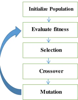
An initial population is created containing a predefined size (number of chromosomes), each represented by a genetic string. Each chromosome has an associated fitness value, typically representing an accuracy value. The concept that fittest (or best) individuals in a population will produce fitter offspring to be used in the next produced population. Selected individuals are choosing for reproduction (or crossover) at each generation; with an appropriate mutation factor to random modify the genes of an individual, in order to develop the new population as shown in Figure 1-2.

Figure 1-2: Overview of simple genetic algorithm Initialize Population Crossover Selection Evaluate fitness Mutation N generations

5

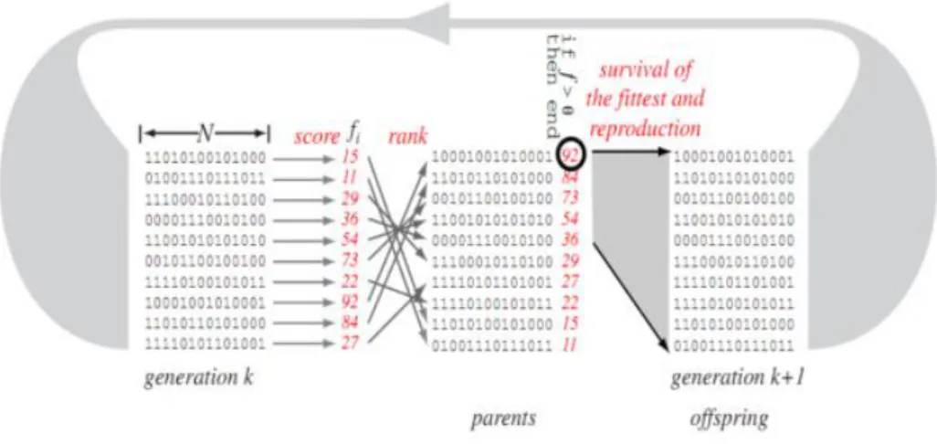
Figure 1-3 shows idea of the basic genetic algorithm. Each of the L subset of features in the population in generation k is representing by a string of bits of length N, called a chromosome. Each classifier is scoured according to its accuracy on a classification task, giving L scalar values.

The chromosomes are then ranked according to this accuracy. The chromosomes are considered in descending order of score, and operated upon by the genetic operators of replication, crossover, and mutation to form the next generation of chromosomes of the offspring. The cycle repeats until a classifier exceeds the higher accuracy.

Figure 1-3: A basic genetic algorithm is a stochastic iterative search method [71]

The GA consists of three main stages: selection, crossover and mutation.

1. Selection (survival of the fittest)

Selection is a genetic operator that chooses a chromosome from the current generation’s population for inclusion in the next generation’s population based on fitness value. For maintained the good results the best chromosomes should survive and create new offspring. To select the best chromosomes, there are many methods for that, such as roulette wheel and rank selection.

2. Crossover

After the selection of the best chromosomes, we will create new population to perform crossover. Crossover selects sub-string (genes) from parent chromosomes and creates a

6

new offspring. The simplest way to do this is to choose randomly some crossover point and everything before this point copy from a first parent and then everything after a crossover point copy from the second parent, as shown in Figure 1-4.

Figure 1-4: The crossover operation in GA [17]

3. Mutation (random modifications)

After a crossover is performed, mutation operator that changes one or more bit values in a chromosome from its initial state. Mutation operator prevent populations to falling into local optimum solutions. For bit-string encoding, we can switch a few randomly chosen bits from 1 to 0 or from 0 to 1. Mutation can then be following, as shown in Figure 1-5:

Figure 7-5: The mutation operation in GA [17]

At the end of the discussion about genetic algorithm improvements, we will list some of the attractive advantages and some disadvantages of genetic algorithms:

Advantages:

 Using chromosome-encoding GA can solve every optimization problem.

7

 Easy to incorporate with other methods.

 Can easily run in parallel.

Disadvantages:

 There is no absolute assurance that a GA will find a global optimum.

 Often computationally expensive, i.e. slow.

 Sometimes it is difficult to find an encoding and a good fitness function.

 The quality of a result is often hard to validate.

1.2.2 Classification Algorithms

The wrapper approach was applied as black box using three classifiers, Artificial Neural Network (ANN), K-Nearest Neighbors (KNN) and J48 Decision tree within optimize search algorithm (Genetic Algorithm).

1.2.2.1Artificial Neural Network (ANN)

Artificial Neural Networks (ANNs) are an attempt to model the power of the brain [1]. The brain has evolved many efficient ways to store and process information that we attempt to model through artificial neural networks.

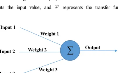
ANN had their start relatively recently in the 1940’s. The basic processing unit of a neural network is the neuron. McCullough and Pitts published the first model of the neuron in 1943 [11]. At the highest level, a neuron receives a series of inputs and depending upon the strength of the input and the connection determines whether the neuron will fire or not. The inputs are multiplying by their synaptic connection and summed. This sum is then using as input for a transfer function, which calculates the output of the neuron. This function is represented by Equation 1-1. The basic conceptual framework for a single neuron is show in Figure 1-6.

8

Where, “w” represents the weight of the synaptic connection between the input and the

neuron, “x” represents the input value, and represents the transfer function of the

neuron.

Figure 1-6: A Simple diagram of a perceptron. Lines represent connections to other neurons (synapses).

The structure of a feed-forward artificial neural network (i.e. multi-layer perceptron) includes input, hidden and output layers see (Figure 1-6). The input layer introduces the distribution of the data for each class to the network. Each input layer node represents one of the input objects features; we will be extracting them from satellite imagery. The output layer is the final processing layer that has a set of values to represent the classes such as (Roads, Buildings, and Rivers).

Training is an iterative process that seeks to modify the network through numerous presentations of data. There are many different methods to train neural networks, the two main distinctions are unsupervised and supervised learning [1]. An unsupervised neural network only uses the input data to adjust its synaptic weights. Supervised learning however relies on a set of training data with known target values. In other words, the training data consists of a set of input patterns and output values. The goal of training is to optimize a function that will map the inputs to the outputs that can be used to correct approximate unseen inputs.

Constructing an ANN using a supervised learning methodology requires the initialization of a network with random synaptic weights between neurons. At this point, an input signal presented to the network would result in no meaningful output. To derive a meaningful output the network synapses must be adjusted. The method to adjust the many weights of the network requires a calculation of error of the network for an input pattern at each epoch. An epoch represents an iteration of measuring the output error and

Input 1 Input 2 Input 3 Output Weight 1 Weight 2 Weight 3

∑

9

updating the synaptic weights in response. A learning rate is often used to control how quickly the weights are updated. If a large value is used the weights of the network will oscillate wildly if set too low it will take more epochs to adjust the weights.

After training is completed, usually signaled by a lack of further decrease in the error or after a set number of epochs, the weights of the network are set and testing of new samples begins. During testing, the testing data is presented to the network to obtain a measure of performance. This performance is measured by a similar method that is using to determine the error of the network during training.

1.2.2.2K-Nearest Neighbors (KNN)

The K-Nearest Neighbors (KNN) algorithm is the most basic instance-based method [41, 31]. KNN is also a lazy learning method where it does not decide how to generalize beyond the training examples until each new input is encountering. In its basic form, the learning phase in IBL algorithms consists of simply saving the normalized feature values of all training instances. With KNN, the classification phase is conducting for a given sample by calculating its pair-wise similarity with all training instances. The similarity is defined by a given similarity function, for example the additive inverse of the Euclidean distance, this function is represented in Equation 1-2. Given a new instance to be classified, its class membership is determining by the most common class of its k nearest neighbors in terms of pair-wise similarities. Because the computation is doing in the classification phase rather than in learning, IBL algorithms are relatively fast at learning but slower at classification [34].

(1-2)

Nearest neighbor, algorithms in general are susceptible to the curse of dimensionality [41]. For an instance to be classified, the predicting region is defined to be the sub-region of the input space containing its k nearest training instances. This formulation leads to a problem when the number of dimensions, n for example, in the input space is large. Because of the geometry of the Euclidean spaces, the radius of the prediction region

11

grows in the proportion of the nth root of the volume whereas the number of training points in the region varies linearly with the volume. Therefore, with large number of features, the variance of the similarities in the predicting regions is high to the proportions that can make the similarity measures misleading.

To overcome this problem, a crucial choice is provided to the k-value. A small k-value can reduce the growth of the volume of the predicting region while a big k-value can

reduce the effect of noise in the data [41].

In addition, feature selection as a means to avoid the problem can be effective with the

nearest neighbors’ classifiers. Because each feature alone is giving the same weight in classification, redundant and irrelevant features can distort the performance of the classifier. An irrelevant feature introduces misleading bias to the similarities and redundant feature causes a particular background concept behind several features to dominate [34].

1.2.2.3J48 Decision tree

Decision Trees are a popular family of supervised learning algorithms. Decision Trees origin from the field of decision and statistics theory [11].

Decision trees are directed graphs with a root, internal nodes, branches and leaves (also known as terminal nodes or decision nodes). All internal and terminal nodes have exactly one incoming branch. The root and the internal nodes have two or more branches leading to their child nodes.

The process of building a tree model from the training set is knows as tree induction or tree growing. The most commonly used approach is the greedy top–down method. The basic idea is to recursively “test on attributes to partition the training data into smaller and smaller subsets until each subset contains instances that belong to a single class” [12].

The general algorithm starts with the entire training set and an empty model. It selects a “best” attribute and generates a node for it. The algorithm performed a test on the attribute’s values and based on the outcome of this test; it partitions the instances at that

11

node in two or more subspaces that are associated to newly created child nodes. This process iterates recursively at each node. The tree induction stops when all instances in a node belong to the same class or if it is not worth to continue partitioning the training data further. Each leaf node has associated a class label, which is the (majority) class of the instances that are associated to that node.

The choice of the best attribute at each node is mainly based on the class distribution of the records before and after the test [21]. Most of the measures used are based on the difference between the degree of impurity at the parent node and the weighted sum of the degrees of impurity at the child nodes after splitting. The relative proportion of instances at the child nodes gives the weights. One common measure of impurity at node t is the entropy, defined as:

(1-3)

Where p (i|t) is the proportion of instances at node t that belong to the class i (i=1,..,c). Other impurity measures are Gini Index and Classification error [35]. When the measure of impurity is entropy, gain is also knows as information gain.

To classify a new instance, this is propagating down the tree and it is labelling accordingly to the class label in the leaf it reaches.

Pruning decision trees is a fundamental step in optimizing the computational efficiency as well as classification accuracy of such a model. Applying pruning methods to a tree usually results in reducing the size of the tree (or the number of nodes) to avoid unnecessary complexity, and to avoid over-fitting of the data set when classifying new data.

There are several decision trees algorithms, such as CHAID [31], CART [6], ID3 [13], C4.5 [14].

12

1.3 Digital Image Processing

Today's with high advanced technology most remote sensing data are recorded and saved in digital format. Digital image processing may involve several procedures including formatting and correcting of the images data, digital enhancement to facilitate better visual interpretation, or even automated classification of targets and features entirely by computer. A digital image that contains graphical information instead of text or a program. Pixels or cells are the basic building blocks of all digital images. Pixels are small adjoining squares in a matrix across the length and width of your digital image as shown in Figure 1-7 [48]. Each cell contain a digital number (DN) this value of each cell is related to the brightness, color or reflectance at that point.

Figure 1-7: Digital image pixels [66]

Most of the common image processing functions available in image analysis systems, which categorized into the following five categories:

1. Preprocessing 2. Image Enhancement 3. Image Transformation 4. Image Segmentation 5. Feature Extraction 1.3.1 Preprocessing

Preprocessing includes data operations, which normally precede further manipulation and analysis of the image data to extract specific information. These operations sometimes

13

referred to as image restoration and rectification, which intended to correct for sensor and platform-specific radiometric and geometric distortions of data [52].

1.3.2 Image Enhancement

Image enhancement is the modification of an image to make it easier for visual interpretation and understanding of imagery. The advantage of digital imagery is that it allows us to manipulate the digital pixel values in an image. Most enhancement operations distort the original digital values [33].

1.3.3 Image Transformation

Digital Image Processing offers a limitless range of possible transformations on remotely sensed data. Image transformations typically involve the manipulation of multiple bands of data, whether from a single multispectral image or from two or more images of the same area acquired at different times (i.e. multitemporal image data) basic image transformations apply simple arithmetic operations to the image data [52]. For more details see Appendix A.2.3.

1.3.4 Image Segmentation

Image segmentation is the primary technique that using to convert a scene or image into multiple objects [33]. Applying the object-based paradigm to image analysis refers to analyzing the image in object space rather than in pixel space, and objects can be used as the primitives for image classification rather than pixels, so image segmentation is the process of partition an image into segments by grouping neighboring pixels with similar feature values (brightness, texture, color, etc.).

1.3.5 Feature Extraction

Feature Extraction uses an object-based method to classify the objects, where an object (also called segment) is a group of pixels with similar spectral, spatial, and/or texture attributes.

After feature extraction, we have three categories of features: spectral feature, spatial feature and texture feature, thus we have 38 features for all categories with three bands

14

for each feature in spectral and texture. We can divide the number of features attributes to 12, 14, and 12 for spectral, spatial and texture respectively.

1.4 Statement of the Problem

In satellite imagery we have 38 features for objects classification and recognition obtained from different features categories (i.e. spectral, texture and spatial). Obtaining the optimum set of features based on genetic algorithm, maintain the classification accuracy and reduce data dimensionality is the main problem of this research. Contrast to previous research, in our work, we need to use extracted features such as spectral, spatial and texture all together.

1.5 Objectives

1.5.1 Main Objective

Increase classification accuracy and reduce data dimensionality for satellite imagery by using GA to select the optimum feature subset.

1.5.2 Specific Objectives

 Literature review

 Use several satellite imagery to take advantage of object features and have more

generalization.

 Design and implement selection of chromosome structure and calculate fitness

function in GA.

 Automated selection of the optimum features subset.

 Evaluate the proposed approach according to classification accuracy.

1.6 Significance of the Thesis

Finding out an optimum set of features for satellite imagery will definitely minimize the computation time and improves the classification accuracy. This helps the experts and specialized software in the field of object recognition to determination an optimal subset of features.

15

1.7 Scope and Limitations

The Satellite imagery contains too many objects such as roads, buildings, trees, rivers and vehicles…etc. Therefore, in this research we intend to extract features only for roads, building and rivers as a data set.

1.8 Methodology

The methodology that will be followed to achieve the study aim can be outlined through the following points.

 Data collection: Aerial photos and satellite images from number of sources that provide these images (Landsat, IKONOS, Spot, and Quick Bird satellites). We downloaded 15 imagery for training and 10 imagery for testing.

 Image processing: Today's with high advanced technology most remote sensing data are recording and saved in digital format. Digital image processing may involve several procedures including formatting and correcting of the images data [13]. In this stage, we need to use ENVI software for image processing.

1. Image Enhancement: Image enhancement is the modification of an image to make it easier for visual interpretation and understanding of imagery. The advantage of digital imagery is that it allows us to manipulate the digital pixel values in an image. Most enhancement operations distort the original digital values.

2. Image Transformation: Digital Image Processing offers a limitless range

of possible transformations on remotely sensed data. Image

transformations typically involve the manipulation of multiple bands of data, whether from a single multispectral image or from two or more images of the same area acquired at different times.

 Image segmentation: The aim of image segmentation is domain-independent partitioning of imagery into a set of visually distinct regions based on properties such as intensity (grey-level), texture, or color [69]. In this stage, we need to use ENVI software for image segmentation.

16

 Feature Extraction: After image segmentation, we need to extract features for each object (Spatial, Texture, and Spectral); also in this stage, we need to use ENVI software.

 Feature Subset Selection (Genetic Algorithm): After extracting the features as a data set, we will use GA as an optimization algorithm to select the best subset of features.

 Evaluation: In this stage, we have many steps to evaluate this work.

1. Extract spatial features only and perform classification accuracy.

2. Extract spectral features only and perform classification accuracy.

3. Extract texture features only and perform classification accuracy.

4. Extract spatial, spectral and texture features all together and perform

classification accuracy.

5. Execute correlation-ranking filter for spatial features only and perform

classification accuracy.

6. After generating features subset using GA, perform classification accuracy

and compare it with others accuracies.

1.9 Outline of the Thesis

The thesis is organized as follows. Chapter 2 present some related works. Chapter 3 includes the methodology and proposed model. In Chapter 4, we present and analyze our experimental results. Chapter 5 will draw the conclusion and summarize the research achievement and future directions.

17

CHAPTER 2: Related works

2.1 Introduction

In the last years, an attention about the feature selection problem has been increasing. In fact, new applications dealing with huge amounts of data have been developing, such as data mining, medical data processing and satellite imagery processing. This chapter intends to give an overview for approaches related to the main topics of this thesis. Generally, when the number of features are large but the number of training samples are small, features that have little or no discriminative information weaken the performance of classifiers. This situation is typically called the curse of dimensionality [58], in this situation we have to choose a feature subset yielding the highest performance.

It is very difficult to predict which features or features combinations will achieve better in classification accuracy. We will have different performances as a result of different features combinations. In addition, using excessive features may degrade the performance of the algorithm and increase the complexity of the classifier. Relatively few features used in a classifier can keep the classification performance robust [16]. Therefore, we have to select an optimized subset of features from a large number of available features.

2.2 Feature Selection Methods

Two major approaches for feature selection, wrapper and filter approach [29, 18, 59, 53]. Many researchers have used wrapper-filter as a hybrid approach [62, 22, 25]. In this thesis, we use wrapper approach for feature selection. In the wrapper approach, the features selection are done using the classification algorithm as a black box. The feature selection algorithm conducts a search for a good subset using the classification algorithm itself as part of the evaluation function. The accuracy of the induced classifiers is estimated using accuracy estimation techniques.

18

2.2.1 Filter Methods

Filter approach evaluate the goodness of the feature subset by using the intrinsic characteristic of the data. As name suggests, filters are algorithms, which filter out insignificant features that have little chance to be useful in analysis of data. Filter methods are computationally less expensive and also more generic than wrappers or furthermore hybrid methods because they do not consider underlying classifier.

Authors in [35] provide an effective feature selection for tree species classifiers in mixed-species of boreal forest. They have one dataset contains 35 input features were the 5 input spectral bands, 9 contextual features and 21 segment-wise features, they have three classes for tree species (pine, spruce and deciduous), and 4 classes for non-tree like shadow, open area (clearance), bare ground and green vegetation. The dataset was splitted in 1/3 for independent testing and 2/3 for model design, with randomly split within each class. Authors provide sequential feature selection with variable ranking and KNN classifier as evaluation technique, which means that measure the correlation between features and classes, this method reduce features from 35 to 10.

2.2.2 Wrapper Methods

Wrapper methods select a feature subset using a learning algorithm as part of the evaluation function. The learning algorithm is used as a kind of “black box” function to guide the search. The evaluation function for each candidate feature subset returns an estimate of the quality of the model that is induced by the learning algorithm, which therefore causes better estimate of accuracy. Wrapper approach based on search algorithms fall into two major categories optimal and suboptimal features subset, such as Sequential Forward Selection, Sequential Backward Selection [23, 55], Sequential Forward Floating Selection and Sequential Backward Floating Selection [40], Steepest Ascent and the Fast Constrained Search [50]. These feature selection techniques have limitations in optimal subset selection for satellite imagery due to strong correlation between features [61].

In recent years, heuristic optimization algorithms such as, genetic algorithm (GA) method [13, 53, 26, 63, 47], ant colony algorithm [61] and swarm intelligent [14, 44], have

19

attracted many attentions in wide range of satellite imagery classification. Many researches works on hyperspectral image, which contain a wealth of data, but interpreting them requires an understanding of exactly what properties of ground materials we are trying to measure, these images contain hundreds of bands and features, many researches work on Hyperspectral images [63, 30].

In [63], authors proposed a GA based wrapper feature selection method “GA-SVM” for hyperspectral imagery, which contains up to 200 bands. Authors used ENVI/IDL as a programming language to implement “GA-SVM”, and they used two criteria to design the fitness function, namely classification accuracy and the number of selected features, to evaluate features subset. For experiments, they create training sets and testing sets using ENVI software labeled with five classes namely built-up area, water body, grassland, forest and unused land. After the experiment, the number of bands used for classification was reduced from 198 to 13, while the classification accuracy increased from 88.81% to 92.51%.

New criterion function called Thornton’s separability index has been successfully deployed for the optimization of feature selection for classification satellite imagery [1, 13, 16]. Thornton’s separability index is defined as the fraction of data points whose classification labels are the same as those of their nearest neighbors. Thus, it is a measure of the degree to which inputs associated with the same output tend to cluster together [16].

Anthony and Ruther in [1] tries to find the optimum combination of bands for every class. They used separability index as evaluation function with Exhaustive Search (ES) and Genetic Algorithm (GA) with SVM as a classification technique, for experiments, they used two datasets with 7 bands and contains six land cover classes were sought namely: wetlands, water (lakes and rivers), Bush/shrub/trees, Grasslands, “bare ground” and Roads. Instead of using classification accuracy to evaluate features subset, they used separability index, to evaluate every band combination. After the experiment, the result can be showed as Roads used two bands (2 & 5), while the classification accuracy increased from 67.22% to 75.32%.

21

Haapanen and Tuominen [24], evaluated the potential of the combination of satellite image (spectral) and aerial photograph (spectral and texture) features to increase classification accuracy for forest inventory. In addition, authors tried to reduce the dimensionality of these features by removing unnecessary or adverse features using two feature selection GA and sequential Forward Selection (FS) with K Nearest Neighbor. Firstly, they use GA and FS to select best features from each image separately are used. Secondly, select best features from combination. Results said the accuracy of the estimation with all features was better than either the satellite image or the aerial photograph features alone.

In [11], authors proposed a method with a three-step object-oriented classification routine that involves the integration of 1) image segmentation, 2) feature selection by GAs and 3) joint Neural Network (NN) based object-classification. For feature extraction, 89 features were extracted using eCognition 3.0 software tool based on IKONOS imagery. After applying feature selection, the dimensionality of the input space is reduced from 89 to 23 and classification accuracy increased from 87.41% to 90.10%.

In [30] authors proposed wrapper approach based on GA as random search technique for subset generation with different classifiers/ induction algorithms namely decision tree C4.5, NaïveBayes, Bayes networks and Radial basis function as subset evaluating criteria on four standard datasets. Experimental results show employing feature subset selection enhanced the classification accuracy in most of the cases. Moreover, results show that no one wrappers among the four wrappers experimented is best for all the datasets experimented.

Ant colony algorithm (ACA) is a cooperative search technique that mimics the foraging behavior of real life ant colonies. Authors in [61] proposed ant colony algorithm for feature selection from hyperspectral imagery. There experiments show that the proposed method reduce the features from 200 to 20.

The goal of authors in [2] is to detect the best spectral band using particle swarm optimization with ANN for supervised classification. For experiments, they used multispectral image with six bands and four classes: road, river, vegetation and urban

21

area. After experiments, the results show that among the red, green and blue bands any one is getting selected in different run of the algorithm.

This paper [38], the impact of genetic search on classification accuracy for rule induction

algorithms is studied. Seven rule induction algorithms: JRip, ConjuctiveRule,

DecisionTable, OneR, PART, Ridor and ZeroR are used based on wrapper approaches. For experiments, 16 input features with 2 output classes are used. After the experiments, genetic search selected four attributes used in rule induction algorithms. Results show that the classification accuracy with genetic search improves or maintains the classifications with the seven rule induction algorithms. Genetic search improves the accuracy of four classifiers: JRip, Ridor, DecisionTable and PART and maintains the accuracy of tree classifiers: ConjuctiveRule, OneR and ZeroR.

2.2.3 Hybrid Filter-Wrapper Methods

The hybrid model attempts to take advantage of the two models by exploiting their different evaluation criteria in different search stages.

In [11], hybrid approach was proposed with Self-adaptive differential evolution (SADE) for searching feature subset and Fuzzy KNN classifier used to calculate the classification accuracy as evaluation criterion. Before doing experiment, authors used ReliefF algorithm for removing the redundancy and noisy of features. After the experiments, the results shown that the SADE based method requires less memory and computation cost than the other searching methods. Authors used GA and Ant Colony Optimization (ACO) based methods for compassion with proposed methods, and the results shown the proposed methods outperforms others.

In [53] authors proposed GA based hybrid feature selection with classification technique called a supervised Nearest Neighbour Distance Matrix (NNDM). WEKA software used for implementation the experiments, which conducted using 9 datasets. The initial population for the feature selection is generated based on Information Gain (IG), which used to generate correlated subset of features, the NNDM classifier used as the evaluation function to evaluate the fitness of the new population. The experiment results show that

22

the proposed method can reduce estimation time needed to optimize the subset feature selection.

2.3 Classification Algorithms

Integrating the GA with other classifiers has been used to produce several feature selection algorithms such as GA-ANN, GA-KNN and GA-J48 Decision tree.

Artificial Neural Network (ANN) used in [22, 30, 4]. Some of the advantages of using ANN, is well suited to problems in which the training data corresponds to noisy and complex sensor data such as satellite imagery. It maintains non-linearity and it could deal with biggest problems. However, it is suffering from multiple local minima; the problem of local minima could be solved by using techniques such as: stochastic gradient descent and k-fold.

K-Nearest Neighbors (KNN) used in [5, 18], KNN classifier is a very simple classifier, it simply uses the training data itself for classification, however it can be slow for real-time prediction if there are a large number of training examples and is not robust to noisy data. Decision tree is used as evaluation classifier in [46, 30, 4]. The main advantage of using decision tree is its simplicity and less sensitivity to errors. However, it is the results candidates to over-fit the training data, especially when the used training data is too small or have noise.

From the above survey, it is noticed that feature selection is of considerable importance, particularly when too many features are used. There are many research works on feature selection using many algorithms and methods, but all of the previous researches never used all the spectral, spatial and texture features all together with 38 features with spectral and texture features with 3 bands. Many of the previous work used one classifier to measure the performance of the new obtained short list of features. In our case, we apply various classifiers to ensure that the results are improving regardless of the classifier type. In addition, some research papers use ACO for feature selection, we preferred to have GA as an optimization algorithm because it is generally known that GA is better in large populations. Moreover, we selected three main objects to consider in our

23

research, i.e., buildings, roads and rivers, roads and rivers haven chosen among the objects because they may look to be very similar and feature selection would be very crucial. To confirm the realistic of our results, we use CRF for spatial features to remove unimportant features and this did not use in previous researches. Overall, the methodology we use is different from all other previous methods as we are going to show in the next chapter.

24

CHAPTER 3: Methodology and Proposed Model

This chapter contains detailed description of the steps of the methodology of our research. The proposed followed methodology is presented below and shown in Figure 3-1.

Figure 3-1 : Methodology flowchart

3.1 Data Collection and Preparation

Maps have been the main source of data for geographic analysis for many years. Raster data is commonly obtained by scanning maps or collecting aerial photographs and

Feature Extraction

Image Processing Image Segmentation

Objects attributes Data Collection

Classification based on features categories

Artificial Ne ural Network (ANN)

K-Nearest Neighbors (KNN) J48 Decision tree Feature Selection GA-ANN GA-KNN GA-J48

Evaluate the subsets

Subsets validation

Artificial Ne ural Network (ANN)

K-Nearest Neighbors (KNN)

25

satellite images. These images are produced from processing high-resolution commercial panchromatic satellite imagery, such as IKONOS, Quickbird2, and Landsat.

3.1.1 Data Collection

Many free sources offer free aerial photos and satellite images in the internet as USGS (U.S. Geological Survey) [61] and NASA website [61].

Many attempts to get suitable aerial and satellite images from various sources to apply feature extraction method have been tried. Some of criteria used to select a case study are diversity of features such as (buildings, trees, roads, and rivers):

1. Number of objects: as shown in Figure 3-4, we chose image contains only Roads and buildings.

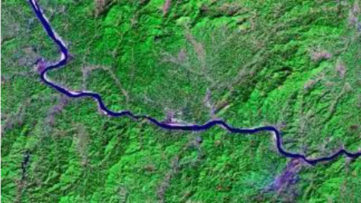
2. Contrasting colors: as shown in Figure 3-2, we chose image contains River as a blue line, which contrasting with the green background.

3. Spatial resolution: as shown in Figure 3-5, we have provide high-resolution image from Gaza municipality for Gaza city.

4. Complexity: as shown in Figure 3-3, we chose image contains asphalt road and land road with convergent colors.

26

Figure 3-3: Sample (2) of satellite image describes asphalt road and land road

Figure 3-4: Sample (3) of satellite image describes asphalt road between buildings

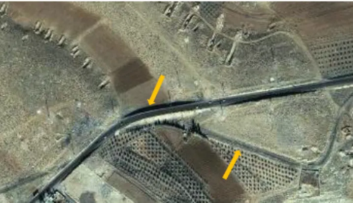
Figure 3-5: Sample (4) of satellite image describes asphalt road between buildings and agricultural area

3.1.2 Image Preprocessing

Preprocessing of an image often include radiometric correction and geometric correction. The following subsections illustrate all needed steps of automatic feature extraction based on sample (4) as shown in Figure 3-5.

27

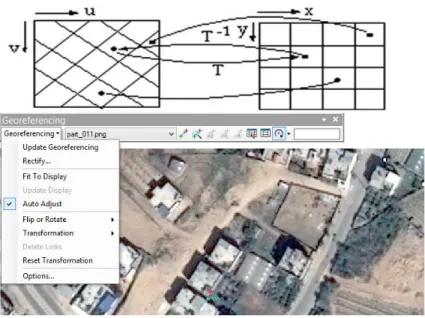
3.1.2.1Geometric Correction

To correct the geometric distortions as we described in Appendix A.2.1, one should apply two steps, geo-referencing and resampling using ARCGIS 10.1 or ERDAS 2013 as shown in Figure 3-6 [33].

The geographic space of each dataset is a reference according to four known coordinates corresponding to the minimum x and y values, the minimum x and maximum y values, the maximum x and minimum y values, and the maximum x and y values. Georeferencing is the process of assigning geographic information to an image. Knowing where an image is located in the world allows information about features contained in that image to be determined. This information includes location, size and distance.

Figure 3-6: Geo-referencing method & toolbar in ARCGIS 10.1

After correcting the coordinate system, the spatial characteristics of pixels may be changed. So resampling should be applied to obtain a new image more pronounced in which all pixels are correctly positioned within the terrain coordinate system to more accurate feature extraction methods.

3.1.2.2Radiometric Correction

Radiometric correction involves the processing of digital images to enhance the accuracy of the brightness value magnitudes. Any imagery contains radiometric errors will be

28

referred to as "noise". These errors should be corrected before the post-processing enhancement, extraction, and analysis of information from the image [2].

The sources of radiometric noise and the appropriate types of radiometric corrections partially depend on the sensor and mode of imaging used to capture the digital image data such as aerial photography, optical scanners, sensors and others.

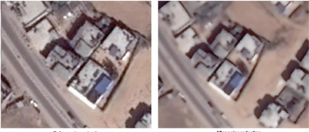
Improvement quality of images, which used in sample (4), radiometric noise reduction, is performed using ERDAS 2013 as shown in Figure 3-7.

Figure 3-7: Noise reduction of sample (4)

3.1.2.3Image Enhancement

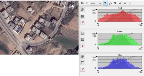
Histogram processing is used in image enhancement. A histogram can tell you whether or not your image has been properly exposed, whether the lighting is harsh or flat, and what adjustments will work best [9], for more details see Appendix A.2.2.

Figure 3-8 showing the image and histogram for study area (sample 4). The histogram shows that the vast majority of the pixels are of medium intensity. Mostly everything in this image is a shade of dark gray. There are, however, several buildings with high intensity.

29

Figure 3-8: Histogram of study area sample (4)

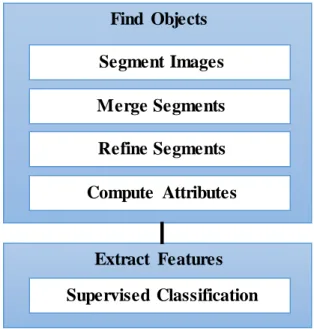
3.2 Feature Extraction Methods

Feature Extraction is a combined process of segmenting an image into objects of pixels, computing attributes for each object, classifying the objects to classes and extract it, for more details see Appendix A.2.5.

Digitizing is a way of conversion of information from analogously produced graphical maps to machine readable vector or raster formats. Many methods are used for the vectorizing process and feature extraction [48]. Automated methods are adopting in this study to extract features from imagery based on object recognition. Figure 3-9