Streamflow Forecasting Using Different Neural Network Models with Satellite Data for a Snow Dominated Region in Turkey

(1)

Procedia Engineering 154 ( 2016 ) 1185 – 1192

Peer-review under responsibility of the organizing committee of HIC 2016 doi: 10.1016/j.proeng.2016.07.526

ScienceDirect

12th International Conference on Hydroinformatics, HIC 2016

STREAMFLOW FORECASTING USING DIFFERENT NEURAL

NETWORK MODELS WITH SATELLITE DATA FOR A SNOW

DOMINATED REGION IN TURKEY

Gökçen Uysal

a

_{*, Ali Arda}

_ù

_orman

a

_{, Aynur}

_ù

_ensoy

a

a_{Civil Engineering, Anadolu University, 2 Eylul Campus, Faculty of Engineering, Department of Civil Engineering, Eski}_ú_{ehir, 26555, Turkey}

Abstract

Data driven models such as Artificial Neural Networks (ANNs) became a very popular tool in hydrology for a long time, especially in rainfall–runoff modelling. However, it does not have common usage in mountainous catchments, where snowmelt plays an important role, due to lack of continuous snow observations. In order to improve the accuracy of snowmelt modeling, recently available satellite snow products are considered as an alternative input to these models. In this study, two different ANN models are employed and compared with each other using novel MODIS satellite snow covered area products as an alternative input into climatic data based models. Firstly, flows are modelled with Multi-Layer Perceptron (MLP) network using gradient-based Levenberg–Marquardt algorithm. Secondly, Radial Basis Function (RBF) network is developed. Both models are performed to estimate the daily flows of Karasu River in the Upper Euphrates Basin, Turkey using 2002 – 2011 data. The main difference between the RBF network and MLP network is in the nature of the nonlinearities associated with hidden nodes. The nonlinearity in MLP is implemented by a fixed function such as a sigmoid. On the other hand, the RBF method bases its nonlinearities on the training set data. In the study the determination of model architectures, optimization algorithms and methods to avoid overfitting are elaborately investigated.

Peer-review under responsibility of the organizing committee of HIC 2016.

Keywords: Upper Euphrates River; streamflow forecasting; neural networks; snowmelt modeling

* Corresponding author. Tel.: +90-222-321-35-50; fax: +90-222-323-95-01. E-mail address: [email protected]

(2)

1. Introduction

Management of water resources are becoming more attractive topic due to growth in population and correspondingly increase in demand to water and energy. Estimation of particularly snowmelt runoff in mountainous basins is coped by modelers using different model sets e.g. conceptual, physical, time series (stochastic) or soft computing models. Due to scarcity of ground observations and uncertainty of model and model parameters across time and space, it is not easily adapt physical models and even sometimes conceptual models may suffer inadequacy of continuous point ground data.

Among various soft computing methods, Artificial Neural Networks (ANNs) are promising tools based on their ability in the modelling of nonlinear processes [1]. Essentially, ANN is a massively parallel-distributed information processing system that has certain performance characteristics resembling biological neural networks of the human brain [2]. It has a flexible mathematical structure that is capable of mapping complex nonlinear relationships between input and output data sets and deriving general trends without describing physical relationships. However, it should not be considered as a mere blackbox [3]. ANNs are able to provide a mapping from one multivariate space to another, given a set of data representing that mapping. Even if the data is noisy and contaminated with errors, ANNs have been known to identify the underlying rule [4]. Thus, ANN has a strong input-output structure and well suited for hydrological models in terms of system estimation and prediction.

Although there have been notable studies on comparison soft computing methods particularly in runoff modeling, they are generally established on rainfall dominated basins [5], [6], [7], [8], [9]. On the other hand, ANN literature is still very limited on snowmelt or snow water equivalent (SWE) modeling [10], [11], [12], [13], [14] due to scarcity of continuous snow data sets. Remote sensing data play key issue to represent change of snow in areal sense. Recently areal snow/SWE satellite data are investigated in hydrology for different aspects e.g. classification of snow products [15], determination of spatial pattern of snow cover duration [16], estimation of fractional snow cover [17] and very recently snowmelting modeling [18]. But, developing alternative data driven models are not well studied in mountainous catchments to estimate flows.

A supervised neural network might be pursued in a number of different ways [2]. While the back-propagation algorithm for the design of a multilayer perceptron (under supervision) may be viewed as an application of stochastic approximation, radial-basis function (RBF) networks can be viewed as a curve-fitting problem in a high-dimensional space. Therefore, each network type has different response to model inputs and has capability of representation of process. In this study, two different ANN models are employed and compared with each other using novel MODIS satellite snow covered area products as an alternative input into climatic data based models particularly for snowmelt modelling in mountainous Upper Euphrates River Basin, Turkey.

2. Study Area and Data

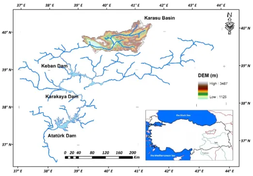
Snow plays a crucial role in the headwaters of Euphrates River Basin as in many other mountainous regions. Snowmelt contributes up to 60–70 % of the annual volume of runoff in the Upper Euphrates River Basin (Karasu Basin), Turkey, during spring and early summer months (March – June). The prediction of snowmelt-induced runoff at the outlet of Karasu Basin has a great potential in water resources management especially for applications in flood forecasting, reservoir management, irrigation, hydropower generation, water supply, since large dam reservoirs exist at the downstream of the basin. Karasu Basin, as one of the major upstream tributaries of Euphrates River, is located at the eastern part of Turkey. Fig.1 shows the location of the basin with its river network. Karasu Basin boundaries are within the longitudes 38o 58ĄE to 41 o 39ĄE and latitudes 39 o 23ĄN to 40 o 25ĄN. The prediction of snowmelt-induced runoff at the outlet of Karasu. The basin has a drainage area of 10,275 km2_{and ranges in altitude}

from 1125 to 3487 m. The main land cover types are pasture, shrub, grass and bareland. The annual mean precipitation of the basin is approximately between 400 and 450 mmyrí1_.

(3)

Fig. 1. Upper Euphrates (Karasu) Basin and location of large dams on Euphrates River

There are totally 18 climatologic and automated weather operating stations (AWOS) ranging in elevation between 981 and 2937 m. Daily average temperature (T) and daily total precipitation (P) values are distributed by Detrended Kriging method [19]; then basin average values are provided as input to the neural network models. For areal snow data, MODIS daily snow product with 500 m spatial resolution is obtained and the time series of SCA (Snow Depletion Curves, SCD) are directly used as an alternative input to models.

3. Methodology

Since operational real time forecasting is targeted for forecasting period, one day before data (n-1) is preferred and used for all data inputs vectors in the model structures. The seasonal model from (01st of March to 30th of June) is preferred using March to July data for ANN based runoff model in applications, since snowmelt constitutes approximately 2/3 of total annual volume of runoff during spring and early summer months. ANN modeling studies have many user defined parts (selection of stopping criteria, normalization techniques, determination of model structure, optimization parameters etc.) in their methodologies, hence several architectures are tested for each model and the best algorithms are selected.

Our approach for both models is firstly to split the data into two sections; the first 70 % of the data for training and the remaining 30 % of the data for validation. Thus the first 7 years (1071 days between 2002 to 2008) are used in the training and the next 3 years (459 days between 2009 to 2011) are used for forecasting (validation). The codes are generated using MATLAB version 2012a software.

3.1. Multi-Layer Perceptron (MLP) network

The one most widely used type of ANN in hydrological studies is the multilayer perceptron (MLP), which is a feedforward network that has interconnected nodes (neurons) arranged into three layers: input layer, a hidden layer and an output layer. The MLP can have more than one hidden layer; however, previous studies have shown that a single hidden layer is sufficient for an ANN to approximate any complex nonlinear function [20]. In this study, a

(4)

two-layer feed-forward artificial neural network structure is constructed with a one-hidden-two-layer. The model has four input vectors, ten neurons in one hidden layers, and one neuron in the output layer (4_10_1_1). The number of neurons in the hidden layer are determined by the trial-and-error procedure. The sigmoid function is employed as an activation function in the training of the network and the learning of the ANN is accomplished by the back-propagation algorithm. Before starting the training process, a random values are assigned for the network weights and biases, respectively. Also, due to the nature of the sigmoid function used in the back-propagation algorithm, it was prudent to standardize all external input and output values before passing them into a neural network; thus input and output vectors are compressed into (0,1) for sigmoid functions..

)

.

(

_j _j

j

f

X

W

b

y

(1) where, X = (x1, . . . , xi, . . . , xn), Wj = (w1j, . . . , wij, . . . , wnj) and X is information from previous nodes, wij

represents the connection weight from the ith_{node in the preceding layer to this node, where b}

j is bias, f is the activation

function. The MLP are optimized using Levenberg-Marquart (LM) algorithm here because this technique is more effective than the conventional gradient techniques [21], [22]. The LM algorithm updates the weights as.

>

T

P

@

T

H

k k

x

J

x

1 1

,

(2) where xk+1 are weights during (k+1)th & kth pass (epoch), J is the Jacobian matrix that contains first derivatives of

the network errors with respect to the weights and biases, μ is learning rate and İ is a vector of network errors. When the scalar μ is zero, this is just Newton's method, using the approximate Hessian matrix. When μ is large, this becomes gradient descent with a small step size. Newton's method is faster and more accurate near an error minimum, so the aim is to shift toward Newton's method as quickly as possible. Thus, μ is decreased after each successful step (reduction in performance function) and is increased only when a tentative step would increase the performance function. In this way, the performance function is always reduced at each iteration of the algorithm. Instead of splitting the first part, a randomly selected 85 % are used for training and 15 % remaining data are used for cross-validation purposes.

3.2. Radial Basis Function (RBF) network

The Radial Basis Function (RBF) network model is motivated by the locally tuned response observed in biological neurons [23]. In the field of mathematical modeling, a radial basis function network is an artificial neural network that uses radial basis functions as activation functions. Contrary to MLP networks with many successive layers, RBF network is composed of three layers. Input layer feeds input signals to the network, middle layer includes RBF functions and output layer is linear combination of all outputs of the RBF layer.

¦

n i i i

R

x

w

u

f

y

1 0

)

(

)

(

(3) where wi = connection weight between the hidden neuron and output neuron; w0 = bias; and x = input vector. A

general class of radial basis functions is described by the Gaussian function given in Equation 4.

)

2 exp(

1 2 2

¦

n i ij i i

c

x

R

V

(4)

(5)

where ܿ௜்= [ci1, ci2, . . . , cin] is the center of the receptive field; ıij is width of the Gaussian function. The major task

of RBF network design is to determine center parameter. Here, a radial basis network one neuron at a time is iteratively created. Neurons are added to the network until the sum-squared error falls beneath an error goal or a maximum number of neurons has been reached using MATLAB 2012a code.

3.3. Evaluation criteria

The performance of the study is tested with 4 criteria defined as the square of correlation coefficient (R) called as coefficient of determination (R2_{), Nash-Sutcliffe Model Efficiency (ME), Root Mean Square Error (RMSE), Mean}

Absolute Error (MAE) denoted as:

2 n 1 t 2 o t o n 1 t 2 m t m n 1 t o t o m t m 2

)

Q

-(Q

)

Q

-(Q

)

Q

-)(Q

Q

-(Q

»

¼

º

«

¬

ª

¦

R

(5)

¦

_n 1 t o t o n 1 t t m t o

)

Q

-(Q

)

Q

-(Q

1 ME

(6)

n

RMSE

¦

n 1 t 2 t o t m

-

Q

)

(Q

(7)

n

MAE

n

¦

t 1 t m t o

-

Q

(8) where is ܳ௠௧ modelled flows, ܳ௢௧is observed flows, ܳത௠is average modelled flows, ܳത௢ is average observed flows, n

is the number of the data sets.

4. Application of models

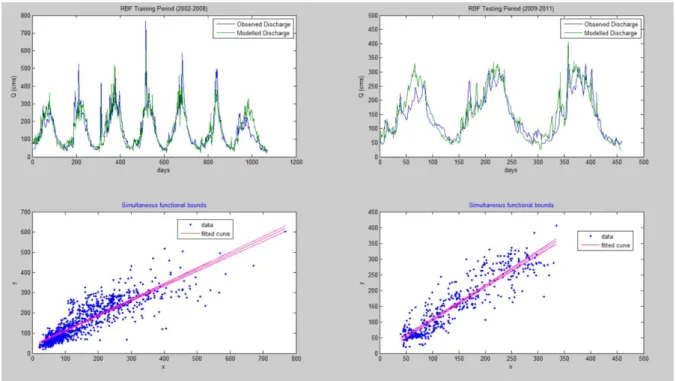
In this part, a comparison is carried out for MLP and RBF networks. Training data are used to determine the weights of network, and a forecasting (testing) part is accomplished for rest of 3 years in order to check the reliability of the model. MLP network is very powerful network for nonlinear relation modeling studies such as snowmelt/rainfall, however in this study, RBF network is also taken into account for same purpose. Both models are trained using 7 years seasonal discharge data from Karasu (Upper Euphrates River) catchment. The input vectors are; precipitation (daily), temperature (daily) and snow covered area which is derived from 500 m resolution MODIS satellite images, and a time index to adjust model results. Both model results are tested with upper and lower 90 % confidence intervals, an example from RBF network modelled discharges vs. observed discharges are shown in Figure 2.

The statistical results are presented in Table 1 in order to compare the network performances. Although, both models have higher correlation regression in validation periods, ME values are relatively less compared to training periods. Also, less RMS errors for validation period in both models may be because of lower stremflows observation within that time. While nonlinearities are associated with sigmoid functions and hidden layer selections in MLP networks, RBF network is capable to identify nonlinearities based on training data sets with radial functions that simplify the separation of the problem solutions. Thus, most challenging and vague part is to select a suitable network type in MLP which is time consuming. Contrary to MLP, RBF is easy to implement with respect to its definite architecture and has less user defined parameters (The training depends on goal and spread selection in MATLAB).

(6)

The performances of the results promote that both model networks can be an alternative model to predict runoff using selected data sets.

Fig. 2. RBF network modelled discharges vs. observed discharges (Training and Test period) with upper and lower 90 % confidence intervals Table 1. Summary table for comparison

Statistical measures Training Forecasting MLP network RBF network MLP network RBF network

R2 _{0.77 0.76 0.83 0.82}

ME 0.77 0.76 0.75 0.73

RMSE (m3_{/s) 51.0 52.5 38.3 39.3}

MAE (m3_/s) _{33.2 34.7 29.0 29.7}

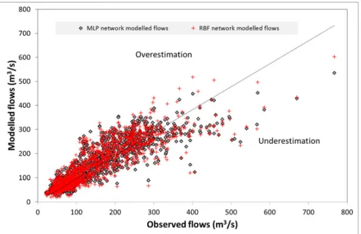
A scatter diagram between modelled and observed flows (Figure 3) is given to show over-and-under estimations. According to that low flows has higher accuracy in both models, mid-flows are underestimated in MLP and overestimated in RBF networks. While high flows are underestimated in both models, RBF network produces higher modelled flows in two peak events.

(7)

Fig. 3. Scatter diagram of two modeled flows vs. observed discharges for whole period.

5. Conclusions and Recommendations

In this study, snowmelt flows in a mountainous region of Turkey (Upper Euphrates River Basin, Karasu) are trained and forecasted by two different neural network approach. Satellite technology provide reliable and areal snow data from which is an alternative input to those models compared to point snow measurements. Besides, the selection of most convenient input combinations in data driven models, comparison of different model structures are essential issue to understand the response of the models. MLP and RBF network based flows are employed using daily meteorological inputs (precipitation and temperature) as well as areal MODIS satellite snow covered product data and compared for 2002 – 2011 March – June periods. The application results indicate that both models give similar results in terms of Nash-Sutcliffe correlation coefficients around 0.75 to 0.74 for training and forecasting, respectively. The networks is better to mimic peak flows compared to MLP structure. Compared to complex method selection of stopping criteria of MLP network, RBF network has less user defined parameters and certain training algorithms which enable for modelers to set simpler networks. In the future works, hybrid models (like ANFIS) may be developed and compared with MLP and RBF network models

Acknowledgements

This study was funded by 1307F284 and 1404F149 Anadolu-BAP and (Scientific Research Project). The authors wish to thank Turkish State Meteorological Service (TSMS) and State Hydraulic Works (DSI) for data contribution.

References

[1] K. Ozgur & H. Sanikhani, Prediction of long䇲term monthly precipitation using several soft computing methods without climatic data, Int. J. Climatol. 35.14 (2015): 4139-4150.

[2] S. Haykin, Neural networks: a comprehensive foundation, Mac-Millan, New York, 1994.

[3] R.S. Govindaraju, Artificial neural networks in hydrology. I: Preliminary concepts, J. Hydrol. Eng. 5.2 (2000): 115-123. [4] R.S. Govindaraju, Artificial neural networks in hydrology: II, hydrologic applications, J. Hydrol. Eng. 5.2 (2000): 124-137.

[5] E. Toth, A. Brath, A. Montanari, Comparison of short-term rainfall prediction models for real-time flood forecasting, J. Hydrol. 239.1 (2000): 132-147.

(8)

[6] Y.M. Chiang, L.C. Chang, F.J. Chang, Comparison of static-feedforward and dynamic-feedback neural networks for rainfall–runoff modeling, J. Hydrol. 290.3 (2004): 297-311.

[7] S. Srinivasulu & A. Jain, A comparative analysis of training methods for artificial neural network rainfall–runoff models, Applied Soft Computing 6.3 (2006): 295-306.

[8] A.P., Piotrowski & J.J. Napiorkowski, A comparison of methods to avoid overfitting in neural networks training in the case of catchment runoff modelling, J. Hydrol. 476 (2013): 97-111.

[9] F., Gökbulak, K. ùengönül, Y. Serengil, ø. Yurtseven, S. Özhan, H. K. Cigizoglu, B. Uygur, Comparison of rainfall-runoff relationship modeling using different methods in a forested watershed, Water Resour. Manag. 29.12 (2015): 4229-4239.

[10] A. S. Tokar, M. Markus, Precipitation-runoff modeling using artificial neural networks and conceptual models, J. Hydrol. Eng. 5.2 (2000): 156-161.

[11] K. Chokmani, T. B. Ouarda, S. Hamilton, M.H. Ghedira, H. Gingras, Comparison of ice-affected streamflow estimates computed using artificial neural networks and multiple regression techniques, J. Hydrol. 349.3 (2008): 383-396.

[12] C.L. Wu, K.W. Chau, Y.S. Li, Predicting monthly streamflow using data䇲driven models coupled with data䇲preprocessing techniques, Water Resour. Res. 45.8 (2009).

[13] S. Abudu, J.P., King, A.S. Bawazir, Forecasting monthly streamflow of spring-summer runoff season in Rio Grande headwaters basin using stochastic hybrid modeling approach. J. Hydrol. Eng., 16(4), 384-390.

[14] V.M. Quiroga, A. Mano, Y. Asaoka, S. Kure, K. Udo, J. Mendoza, Snow glacier melt estimation in tropical Andean glaciers using artificial neural networks, Hydrol. Earth Syst. Sc. 17.4 (2013): 1265-1280.

[15] J.J. Simpson & T.J. McIntire, A recurrent neural network classifier for improved retrievals of areal extent of snow cover, Geoscience and Remote Sensing, IEEE Transactions on 39.10 (2001): 2135-2147.

[17] I.D. Dobreva & A.G. Klein, Fractional snow cover mapping through artificial neural network analysis of MODIS surface reflectance, Remote Sens. Environ. 115.12 (2011): 3355-3366.

[18] M. Ataৢ, A.E. Tekeli, S. Dönmez, H. Fouli, Use of interactive multisensor snow and ice mapping system snow cover maps (IMS) and artificial neural networks for simulating river discharges in Eastern Turkey, Arab. J. Geosci. 9.2 (2016): 1-17.

[19] D.C. Garen & D. Marks, Spatially distributed energy balance snowmelt modelling in a mountainous river basin: estimation of meteorological inputs and verification of model results, J. Hydrol. 315.1 (2005): 126-153.

[20] G. Cybenco, Approximation by superpositions of a sigmoidal function, Math. Cont. Signal. 2.4 (1989): 303-314.

[21] M.T. Hagan & M.B. Menhaj, Training feedforward networks with the Marquardt algorithm, Neural Networks, IEEE Transactions on 5.6 (1994): 989-993.

[22] Ö. Kiúi, Daily pan evaporation modelling using multi䇲layer perceptrons and radial basis neural networks, Hydrol. Process. 23.2 (2009): 213-223.