David J. Friedlander
Glenn Research Center, Cleveland, Ohio
Understanding the Flow Physics of
Shock Boundary-Layer Interactions
Using CFD and Numerical Analyses
NASA/TM—2013-218081
NASA STI Program . . . in Profi le
Since its founding, NASA has been dedicated to the advancement of aeronautics and space science. The NASA Scientifi c and Technical Information (STI) program plays a key part in helping NASA maintain this important role.
The NASA STI Program operates under the auspices of the Agency Chief Information Offi cer. It collects, organizes, provides for archiving, and disseminates NASA’s STI. The NASA STI program provides access to the NASA Aeronautics and Space Database and its public interface, the NASA Technical Reports Server, thus providing one of the largest collections of aeronautical and space science STI in the world. Results are published in both non-NASA channels and by NASA in the NASA STI Report Series, which includes the following report types:
• TECHNICAL PUBLICATION. Reports of completed research or a major signifi cant phase of research that present the results of NASA programs and include extensive data or theoretical analysis. Includes compilations of signifi cant scientifi c and technical data and information deemed to be of continuing reference value. NASA counterpart of peer-reviewed formal professional papers but has less stringent limitations on manuscript length and extent of graphic presentations.
• TECHNICAL MEMORANDUM. Scientifi c and technical fi ndings that are preliminary or of specialized interest, e.g., quick release reports, working papers, and bibliographies that contain minimal annotation. Does not contain extensive analysis.
• CONTRACTOR REPORT. Scientifi c and technical fi ndings by NASA-sponsored contractors and grantees.
• CONFERENCE PUBLICATION. Collected papers from scientifi c and technical
conferences, symposia, seminars, or other meetings sponsored or cosponsored by NASA. • SPECIAL PUBLICATION. Scientifi c,
technical, or historical information from NASA programs, projects, and missions, often concerned with subjects having substantial public interest.
• TECHNICAL TRANSLATION. English-language translations of foreign scientifi c and technical material pertinent to NASA’s mission. Specialized services also include creating custom thesauri, building customized databases, organizing and publishing research results.
For more information about the NASA STI program, see the following:
• Access the NASA STI program home page at http://www.sti.nasa.gov
• E-mail your question to [email protected] • Fax your question to the NASA STI
Information Desk at 443–757–5803 • Phone the NASA STI Information Desk at 443–757–5802
• Write to:
STI Information Desk
NASA Center for AeroSpace Information 7115 Standard Drive
David J. Friedlander
Glenn Research Center, Cleveland, Ohio
Understanding the Flow Physics of
Shock Boundary-Layer Interactions
Using CFD and Numerical Analyses
NASA/TM—2013-218081
National Aeronautics and
Space Administration
Glenn Research Center
Cleveland, Ohio 44135
Acknowledgments
The author would like to acknowledge the support from the Air Force Research Laboratory, Air Vehicle Directorate, AFRL/RB and the interaction with the U.S. Air Force Collaborative Center for Aeronautical Sciences as well as the NASA Fundamental Aeronautics Program for supporting this research. The author would also like to thank NASA’s High End Computing Program (HECC) for providing super-computing resources that were vital in this endeavor. Also appreciated is the base grid (of which all grids used in this thesis were derived from) and grid modifi cation codes that were developed by Marshall Galbraith and guidance from Daniel Galbraith. A special thanks goes to Dr. Mark Turner, Dr. Paul Orkwis, and Dr. Nicholas Georgiadis for all their guidance and support with this thesis work.
Available from NASA Center for Aerospace Information
7115 Standard Drive Hanover, MD 21076–1320
National Technical Information Service 5301 Shawnee Road Alexandria, VA 22312 Trade names and trademarks are used in this report for identifi cation
only. Their usage does not constitute an offi cial endorsement, either expressed or implied, by the National Aeronautics and
Space Administration.
Abstract
Mixed compression inlets are common among supersonic propulsion systems. However they are susceptible to total pressure losses due to shock/boundary-layer interactions (SBLI's). Because of their importance, a workshop was held at the 48th American Institute of Aeronautics and Astronautics (AIAA) Aerospace Sciences Meeting in 2010 to gauge current computational uid dynamics (CFD) tools abilities to predict SBLI's. One conclusion from the workshop was that the CFD consistently failed to agree with the experimental data. This thesis presents additional CFD and numerical analyses that were performed on one of the congurations presented at the workshop.
The additional analyses focused on the University of Michigan's Mach 2.75 Glass Tunnel with a semi-spanning 7.75 degree wedge while exploring key physics pertinent to modeling SBLI's. These include thermodynamic and viscous boundary conditions as well as turbulence modeling. Most of the analyses were 3D CFD simulations using the OVERFLOW ow solver. However, a quasi-1D MATLAB code was developed to interface with the National Institute of Standards and Technology (NIST) Reference Fluid Thermodynamic and Transport Properties Database (REFPROP) code to explore perfect verses non-ideal air as this feature is not supported within OVERFLOW. Further, a grid resolution study was performed on the 3D 56 million grid point grid which was shown to be nearly grid independent. Because the experimental data was obtained via particle image velocimetry (PIV), a fundamental study pertaining to the eects of PIV on post-processing data was also explored.
Results from the CFD simulations showed an improvement in agreement with experimental data with certain settings. This is especially true of the v velocity eld within the streamwise data plane. Key
contributions to the improvement include utilizing a laminar zone upstream of the wedge (the boundary-layer was considered transitional downstream of the nozzle throat) and the necessity of mimicking PIV particle lag for comparisons. It was also shown that the corner ow separations are highly sensitive to the turbulence model. However, the center ow region, where the experimental data was taken, was not as sensitive to the turbulence model. Results from the quasi-1D simulation showed that there was little dierence between perfect and non-ideal air for the conguration presented.
Understanding the Flow Physics of Shock Boundary-Layer
Interactions Using CFD and Numerical Analyses
David J. Friedlander
National Aeronautics and Space Administration Glenn Research Center
Table of Contents
Abstract ii
List of Figures viii
List of Tables xiii
Nomenclature xiv
1 Background 1
1.1 Introduction . . . 1
1.2 Experimental Research Literature Survey . . . 3
1.3 Computational Research Literature Search . . . 4
2 Geometry and Numerical Modeling 10 2.1 Geometry and Mesh . . . 10
2.2 Solver . . . 13
3 Case Overviews 15 3.1 CFD Cases with OVERFLOW . . . 15
3.2 PIV Exploration . . . 18 4 Flat Plate 20 4.1 Overview . . . 20 4.2 Results . . . 21 5 Quasi-1D Code 24 5.1 Overview . . . 24
5.2 Calorically Perfect Code . . . 25
5.3 Non-Ideal Code . . . 28
5.4 Quasi-1D Exploration . . . 31
6 Grid Resolution Study 33
7 Results 37
7.1 Standard Case . . . 37
7.2 Particle Lag Eects . . . 38
7.3 Isothermal Case . . . 41
7.4 Trip Case . . . 45
7.5 Turbulence Modeling Eects . . . 47
7.6 Metrics . . . 50 7.7 Blockage Revisited . . . 54 8 Conclusions/Future Work 56 References 58 A Velocity Contours 64 B Velocity Proles 68 B.1 Standard Case . . . 68 B.2 Combined Case . . . 71
B.3 Modied Geometry, Isothermal, and Trip Cases . . . 74
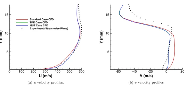
B.4 TKE and MUT Cases . . . 77
B.5 Standard Case with Various Turbulence Models . . . 80
C Combined Case with Various Turbulence Models 83 D Shock Angle Calculation 88 E Simulation Checklists 91 E.1 Initial . . . 91
E.2 Standard Case . . . 92
E.3 Isothermal Case . . . 93
E.4 Modied Geometry Case . . . 94
E.5 All-Laminar Case . . . 95
E.6 Trip Case . . . 96
E.7 Combined Case . . . 97
E.8 TKE Case . . . 98
E.10 Standard Case with SST-GY . . . 100
E.11 Standard Case with BSL . . . 101
E.12 Flat Plate with SST . . . 102
E.13 Flat Plate with K-Omega . . . 103
E.14 Flat Plate with SST-GY . . . 104
List of Figures
1 A supersonic mixed compression inlet (used with permission from Pitt Ford and Babinsky [1]). 1 2 Sketch of the oblique shock / boundary-layer interaction (used with permission from Touber
and Sandham [2]). . . 1 3 Iso-surfaces of density gradients in the downstream direction around the wedge, colored by
the derivative of the density gradients in the downstream direction (from Galbraith [3]). . . . 2 4 Datum groove, 8mm wide groove and variations (from Holden and Babinsky [4]). . . 3 5 Three-dimensional bumps (from Holden and Babinsky [4]). . . 4 6 Velocity proles 94 mm downstream of micro-ramp controlled SBLI, h = 3 mm (used with
permission from Pitt Ford and Babinsky [1]). . . 4 7 Mach number contours of the converged mesoap array simulations, (used with permission
from Ghosh et al. [5]). . . 5 8 Contours of the skin friction coecient of a at plate SBLI with time averaged (top) and
instantaneous (bottom) snapshots (from Morgan et al. [6]). . . 6 9 Comparison of RANS and LES results on a square duct (from Medic et al. [7]). . . 6 10 Congurations run with DNS, LES, and RANS (used with permission from Knight et al. [8]). 7 11 Flow pattern sketches for the experiment (left) and DNS (right) for a 24 degree compression
corner (from Wu et al. [9]). . . 8 12 Comparison of the size of the separation bubble with (new) and without (old) a dissipation
limiter (from Wu and Martin [10]). . . 8 13 Skin friction distribution (RANS models) for a 28 degree compression corner at Mach 5 (used
with permission from Edwards et al. [11]). . . 9 14 Cut-away view of the University of Michigan Glass Tunnel (from Lapsa [12]). . . 10 15 Schematic of the University of Michigan Glass Tunnel with upstream ow straightener and
seeder (from Lapsa [12]). Note units are in inches. . . 11 16 7.75 degree wedge geometry. Dimensions courtesy of Lapsa [12]. . . 11 17 Grid throat region packing with original (left) and nal (right). . . 12 18 Side view of the grid representing the tunnel and 7.75 degree wedge with center-span wedge
and throat inserts shown. . . 12 19 Sample modied nozzle contour. Note the dierence between the old and new throat heights
is exaggerated compared to what was actually used. . . 16 20 Momentum thickness Reynolds number at the bottom wall (half-span) for the laminar case. . 17
21 Momentum thickness Reynolds number at the bottom wall, center-span. . . 17
22 Measured particle response through an oblique shock (from Lapsa [12]). The velocity com-ponent normal to the shock,un, is normalized by the pre-shock (un1) and post-shock (un2) velocities and shown as a function of the shock-normal direction,n. An exponential t to the data reveals the particle relaxation time,τ p= 5.5 µs. . . 19
23 Flat plate 2D grid and boundary conditions [13]. . . 20
24 Skin friction coecient proles. . . 21
25 u+ verses y+ for the various turbulence models at Re x= 4.2E6. . . 22
26 Normalized turbulent parameters for various turbulence models atRex= 4.2E6 . . . 23
27 Normalized turbulent parameters at various freestream turbulent viscosities atRex= 4.2E6 . 23 28 Sample enthalpy verses entropy diagram for calculating across an oblique shock for a non-ideal gas. 1: total conditions at Station 1, 1S: static conditions at Station 1, 2S: static conditions at Station 2, 2: total conditions at Station 2. . . 24
29 Oblique shock notation. . . 25
30 Percentage dierences between non-ideal and perfect air for various parameters. . . 32
31 Percentage dierences of the shock angle between non-ideal and perfect air for varying wedge angles. . . 32
32 Streamwise cross-sections at center-span for the various grid levels. . . 33
33 L2 residuals for the Standard case. . . 34
34 uvelocity proles within the streamwise plane. . . 35
35 Data plane location in reference to the grid. . . 37
36 u velocity (left) and v velocity (right) streamwise contours for the experiment (top) and Standard case (bottom). . . 38
37 Bottom wall separation underneath the wedge for the Standard case. . . 38
38 v velocity streamwise contours for the experiment (top), short lag (middle-top), medium lag (middle-bottom), and long lag (bottom). . . 39
39 Select velocity proles at the most-upstream axial location (x= 18.191mm) for the Standard case. . . 40
40 Select velocity proles at the rst intersecting spanwise plane (x= 20.76mm) for the Standard case. . . 40
41 Select velocity proles at the most-upstream axial location (x= 18.191mm) for the Combined case. . . 41
42 Select velocity proles at the rst intersecting spanwise plane (x= 20.76 mm) for the
Com-bined case. . . 41
43 Freestream thermal boundary-layer at x = −63.9 mm. Temperature cut o is at 99% freestream (121.2 K). . . 42
44 Temperature proles at the most-upstream axial location (x= 18.191mm). . . 43
45 Total temperature centerspan prole at the bottom wall with the following stations marked: 1. Throat, 2. Trip location, 3. Start of the tunnel straight section, 4. Wedge leading edge, 5. Wedge trailing edge. . . 43
46 Select velocity proles at the most-upstream axial location (x= 18.191 mm). . . 44
47 uvelocity dierence contours. . . 44
48 v velocity dierence contours. . . 44
49 Static temperature dierence contours. . . 45
50 Select velocity proles at the most-upstream axial location (x= 18.191 mm). . . 45
51 Select velocity proles at the rst intersecting spanwise plane (x= 20.76mm). . . 46
52 Turbulent kinetic energy proles. . . 46
53 Select velocity proles at the most-upstream axial location (x= 18.191 mm). . . 47
54 Select velocity proles at the rst intersecting spanwise plane (x= 20.76mm). . . 48
55 Turbulent kinetic energy proles. . . 48
56 Velocity proles at the most-upstream axial location (x= 18.191mm) for various turbulence models, Standard Case. . . 49
57 Velocity proles at the rst intersecting spanwise plane (x= 20.76mm) for various turbulence models, Standard Case. . . 49
58 Bottom wall separation underneath the wedge for the Standard case with various turbulence models. . . 50
59 Point locations within the centerspan plane. Mach number contour of the Standard case CFD solution is shown. . . 52
60 Shock angle verses Mach number. . . 53
61 Bottom wall separation underneath the wedge for the Isothermal and Modied Geometry cases. 54 62 Bottom wall separation underneath the wedge for the Trip and Combined cases. . . 55
A.1 uvelocity contours for the Standard (left) and Combined (right) cases with lag. . . 64
A.2 u(left) andv (right) velocity contours for Isothermal and Modied Geometry cases. . . 65
A.3 u(left) andv (right) velocity contours for Trip and Combined cases. . . 65
A.5 u(left) andv (right) velocity contours for the Standard case with SST-GY and BSL. . . 66
A.6 u(left) andv (right) velocity contours for the Combined case with SST-GY and BSL. . . 67
B.1 Velocity proles atx= 26.76mm, Standard case. . . 68
B.2 Velocity proles atx= 30.76mm, Standard case. . . 68
B.3 Velocity proles atx= 34.76mm, Standard case. . . 69
B.4 Velocity proles atx= 38.76mm, Standard case. . . 69
B.5 Velocity proles atx= 41.76mm, Standard case. . . 70
B.6 Velocity proles atx= 53.76mm, Standard case. . . 70
B.7 Velocity proles atx= 26.76mm, Combined case. . . 71
B.8 Velocity proles atx= 30.76mm, Combined case. . . 71
B.9 Velocity proles atx= 34.76mm, Combined case. . . 72
B.10 Velocity proles atx= 38.76mm, Combined case. . . 72
B.11 Velocity proles atx= 41.76mm, Combined case. . . 73
B.12 Velocity proles atx= 53.76mm, Combined case. . . 73
B.13 Velocity proles atx= 26.76mm, various cases. . . 74
B.14 Velocity proles atx= 30.76mm, various cases. . . 74
B.15 Velocity proles atx= 34.76mm, various cases. . . 75
B.16 Velocity proles atx= 38.76mm, various cases. . . 75
B.17 Velocity proles atx= 41.76mm, various cases. . . 76
B.18 Velocity proles atx= 53.76mm, various cases. . . 76
B.19 Velocity proles atx= 26.76mm, TKE and MUT cases. . . 77
B.20 Velocity proles atx= 30.76mm, TKE and MUT cases. . . 77
B.21 Velocity proles atx= 34.76mm, TKE and MUT cases. . . 78
B.22 Velocity proles atx= 38.76mm, TKE and MUT cases. . . 78
B.23 Velocity proles atx= 41.76mm, TKE and MUT cases. . . 79
B.24 Velocity proles atx= 53.76mm, TKE and MUT cases. . . 79
B.25 Velocity proles atx= 26.76mm, Standard case with various turbulence models. . . 80
B.26 Velocity proles atx= 30.76mm, Standard case with various turbulence models. . . 80
B.27 Velocity proles atx= 34.76mm, Standard case with various turbulence models. . . 81
B.28 Velocity proles atx= 38.76mm, Standard case with various turbulence models. . . 81
B.29 Velocity proles atx= 41.76mm, Standard case with various turbulence models. . . 82
B.30 Velocity proles atx= 53.76mm, Standard case with various turbulence models. . . 82
C.2 Velocity proles atx= 20.76mm, Combined case with various turbulence models. . . 84
C.3 Velocity proles atx= 26.76mm, Combined case with various turbulence models. . . 84
C.4 Velocity proles atx= 30.76mm, Combined case with various turbulence models. . . 85
C.5 Velocity proles atx= 34.76mm, Combined case with various turbulence models. . . 85
C.6 Velocity proles atx= 38.76mm, Combined case with various turbulence models. . . 86
C.7 Velocity proles atx= 41.76mm, Combined case with various turbulence models. . . 86
C.8 Velocity proles atx= 53.76mm, Combined case with various turbulence models. . . 87
C.9 Bottom wall separation underneath the wedge for the Combined case with various turbulence models. . . 87
D.1 Shock angle diagram/nomenclature. . . 89
D.2 Velocity proles for determining shock line end location (Standard case shown). . . 89
D.3 Arc length prole for determining shock line end location (Standard case shown). . . 89
List of Tables
1 Summary of CFD Cases. . . 18
2 Various ow parameters used to determine grid convergence. . . 35
3 Mass ow rates (kg/s) used to determine grid convergence. . . 35
4 Coordinates for grid resolution study. . . 36
5 Workshop error metric comparisons. . . 51
6 uvelocity and velocity dierences. . . 52
Nomenclature
Acronyms
AGS Abu-Ghannam and Shaw
AIAA American Institute of Aeronautics and Astronautics CFD Computational Fluid Dynamics
DNS Direct Numerical Simulation LES Large-Eddy Simulation
NIST National Institute of Standards and Technology PIV Particle Image Velocimetry
RANS Reynolds-Averaged Navier-Stokes SBLI Shock Boundary Layer Interaction SST Shear Stress Transport
UM University of Michigan VG Vortex Generator
a speed of sound
A/A∗ geometric throat area ratio
b∗ throat blockage parameter
C constant
cf skin friction coecient
cp specic heat at constant pressure
E(f) error metric off e(f)n local error off f function/lookup
i,n index
k turbulent kinetic energy L length scale
l arc length
M Mach number
m power coecient
˙
m∗ geometric throat mass ow rate
p pressure
R specic gas constant rc thermal recovery factor
Re Reynolds number
s entropy
T temperature
u,v streamwise and transverse velocity components V velocity
x,y,z cartesian coordinates
˜
x,y˜ adjusted cartesion coordinates
y+,u+ wall coordinates
Greek Symbols
β shock angle
γ ratio of specic heats θ turning/wedge angle κ Von Karmin constant µ dynamic viscocity
ρ density τ time constant
Subscripts
1 upstream
2 downstream
∞,Inf freestream condition
n normal
ref reference condition
∗ sonic condition
T turbulent
1 Background
1.1 Introduction
Mixed compression inlets are often found in supersonic aircraft propulsion systems with a typical mixed compression inlet shown in Fig. 1. These inlets are susceptible to shock boundary-layer interactions (SBLI) with a typical SBLI shown in Fig. 2. As one can see, SBLI's are not trivial in nature and beyond the situation shown in Fig. 2, are very three dimensional ows, shown in Fig. 3. SBLI's are a concern for supersonic aircraft propulsion system designs as the separation induced by the shock interacting with the turbulent boundary-layer results in a total pressure loss that is not accounted for in inviscid theory. As mixed compression inlets become more at the forefront of aviation technology, it becomes crucial to understand SBLI's and how they aect propulsion system performance. This can be achieved in several ways, including fundamental and ow control experiments as well as computational work, all of which will be discussed further in the next sections.
Figure 1: A supersonic mixed compression inlet (used with permission from Pitt Ford and Babinsky [1]).
Figure 2: Sketch of the oblique shock / boundary-layer interaction (used with permission from Touber and Sandham [2]).
Figure 3: Iso-surfaces of density gradients in the downstream direction around the wedge, colored by the derivative of the density gradients in the downstream direction (from Galbraith [3]).
In order to determine how eectively computational uid dynamics (CFD) tools can currently pre-dict SBLI's, a workshop was held at the 48th American Institute of Aeronautics and Astronautics (AIAA) Aerospace Sciences Meeting featuring an array of CFD analyzes [14, 15, 16] with experimental data sets provided by the Institut Universitaire des Systemes Thermiques Industriels [17] and the University of Michi-gan (UM) [18]. The CFD results from the workshop are summarized in DeBonis et al. [19] with workshop conclusive remarks documented in works by Benek et al. [20, 21] as well as Hirsch [22]. One key conclusion of the workshop was that the CFD analyses failed to match experimental data. Because of the complex nature of SBLI's, it is of great interest within the aero-propulsion and CFD communities to see if there are ways to improve CFD methods or more eectively use existing methods. This will enable better prediction of SBLI's as well as aid in future inlet design.
Thus further CFD analyses were performed at the University of Cincinnati's Gas Turbine Simulation Laboratory as a compliment to work done by Galbraith [3, 23] in hopes to better understand the compu-tational factors involved in calculating SBLI's as well as to explore alternatives to the error metric used in the workshop. One of the data sets provided to the workshop by UM was their Glass Tunnel with a semi-spanning 7.75 degree wedge at a freestream Mach number of 2.75. The UM experimental data was obtained using stereo particle image velocimetry (PIV) techniques [18]. The CFD analyses presented here focus on that particular UM case while exploring various key physics associated with SBLI's, including, but not limited to, heat transfer boundary conditions, geometry sensitivities, laminar verses turbulent ow assumptions, and turbulence modeling. Special attention was paid to the u and v velocity components,
particularly around the oblique shock o the leading edge of the wedge. This is because it was felt that the CFD and post-processing calculations from the workshop missed the peakuvelocity as well as the location
of the shock as dened by thev velocity prole. If the upstream proles are not in agreement, it is fair to
say that the solutions downstream should not agree. Aside from the CFD cases, a preliminary exploration into the eects on PIV obtained data is also presented.
1.2 Experimental Research Literature Survey
The workshop was not the rst and certainly not the last time SBLI's have been examined both experimen-tally and numerically. Experiments by Holden and Babinsky [4] attempted SBLI ow control via a series of streamwise grooves and bumps, shown in Figs. 4 and 5, with hopes of smearing the shock footprint. They showed that the ow elds inherent with SBLI's are highly sensitive to geometry deviations, such as the slot and bump geometries, or for that matter any foreign debris or geometry imperfections. Another experiment by Holden and Babinsky [24] explored the use of vortex generators (VG's) for SBLI ow control. Two types were tested: wedge-shaped, more commonly known as micro-ramps, and counter rotating vanes. It was found that the use of the VG's greatly reduced the separation region of the SBLI interaction region, with the vane type VG's going as far as to eliminate the separation region completely. Experiments by Pitt Ford and Babinsky [1] as well as by Lapsa [12] also explored the eects of micro-ramps on SBLI ow elds. Pitt Ford and Babinsky showed that micro-ramps located upstream of the interaction region can break up the separation bubble but not completely eliminate it while increasing downstream velocities, shown in Fig. 6. Lapsa showed that the use of inverse micro-ramps can decrease the displacement thickness and thus allow for less separation around the interaction region.
Figure 5: Three-dimensional bumps (from Holden and Babinsky [4]).
Figure 6: Velocity proles 94 mm downstream of micro-ramp controlled SBLI, h = 3 mm (used with per-mission from Pitt Ford and Babinsky [1]).
While the above mentioned experiments focused mostly on ow control, more fundamental experiments have been performed in order to understand the nature of SBLI's. An experiment performed by Babinsky et al. [25] explored the importance of corner ows in relation to SBLI's. They showed that the corner ow separations have a coupled eect with the separation bubble of the interaction region of SBLI's. Thus by decreasing the corner ow separation it was shown that the interaction region separation would be reduced and approach a 2D nature. This coupling nature was also shown in a prior experiment by Titchener et al. [26].
1.3 Computational Research Literature Search
Over the years there have been plenty of numerical simulations exploring all facets of SBLI's: from ow control to numerical modeling eorts. For ow control, Ghosh et al. [5] investigated the use of aeroelastic mesoaps via two and three dimensional simulations, shown in Fig. 7. The simulations utilized both
Reynolds-Averaged Navier-Stokes (RANS) and Large-Eddy/Reynolds-Averaged Navier-Stokes (LES/RANS) means for solving the ow equations. The simulations showed that the use of mesoaps for ow control resulted in a slightly larger interaction region compared to the non-controlled case.
Figure 7: Mach number contours of the converged mesoap array simulations, (used with permission from Ghosh et al. [5]).
Morgan et al. [6] performed LES simulations with a at plate geometry to explore SBLI's. An instanta-neous as well as time-averaged snapshot of the skin friction coecient within the interaction region is shown in Fig. 8. It can be seen that the time-averaged snapshot greatly smooths out the chaotic nature of the SBLI, including the separation region. In fact, the instantaneous snapshot shows that the separation region consists of many separation bubbles and not just a single separation zone as shown in the time-averaged snap shot. This is important as steady RANS simulations only have the capability to reproduce time-averaged behavior unlike LES instantaneous solutions. The comparison between LES and RANS solutions were fur-ther explored by Medic et al. [7] using a simple square duct with results shown in Fig. 9. It can be seen that the RANS solution over predicts the boundary layer growth at the duct corners relative to the LES solution. This over prediction can have a tremendous eect in SBLI simulations, especially when using a tunnel-like geometry, due to the coupling eects between the corner ows and interaction region separation discussed earlier. Other LES solution eorts have been conducted by Hunt and Nixon [27], based on experimental data obtained by Dolling and Murphy [28], as well as by Jamalamadaka et al. [29].
Figure 8: Contours of the skin friction coecient of a at plate SBLI with time averaged (top) and instan-taneous (bottom) snapshots (from Morgan et al. [6]).
Figure 9: Comparison of RANS and LES results on a square duct (from Medic et al. [7]).
Further, a series of simulations were performed by Knight et al. [8] exploring SBLI's. Five congurations were run, shown in Fig. 10, and utilized Direct Numerical Simulations (DNS), LES, and RANS. There were a multitude of lessons learned from these simulations, especially regarding the RANS simulations. With RANS, the case of the 3D single n correctly predicted the secondary separation region with use of the Wilcox-Durbin model. However, the RANS simulation of the 3D double n failed to accurately predict the surface heat transfer using the linear and weakly non-linear Wilcox-based models. This is common for RANS simulations of SBLI ows, as also shown by simulations conducted by Knight and Degrez [30]. Other overviews of SBLI simulations involving DNS, LES, and LES/RANS methods can be found in works by
Zheltovodov [31] and Edwards [32], the latter of which touches briey on experiments exploring the eects of heat transfer on SBLI's by Zheltovodov et al. [33, 34].
Figure 10: Congurations run with DNS, LES, and RANS (used with permission from Knight et al. [8]). Wu et al. [9, 35, 36, 37, 10, 38, 39] have performed a series of DNS simulations on a 24 degree compression ramp with experimental data provided by Bookey et al. [40]. Originally they showed that the DNS simu-lations under predicted the separation region within the SBLI interaction, as shown in Fig. 11. Numerical code bugs as well as the incoming conditions to the corner were eliminated as factors of the discrepancy due to the agreement between the DNS simulation and the experimental data upstream of the compression corner. In turn, they determined that numerical modeling of SBLI's is sensitive to the numerical dissipation and suggested the use of a limiter on the dissipation schemes. Rerunning the DNS simulations with the limiter showed great improvements in predicting the size of the separation region, shown in Fig. 12.
Continuing with the compression corner theme, Edwards et al. [11] used LES/RANS to explore a 28 degree compression corner ow interaction. Menter's Shear Stress Transport (SST) [41] turbulence model was used for the RANS portion. Although the simulations captured the shock behavior well, it was noted that there was a great dependence on the shear stress transport limiter within the SST turbulence model, shown in Fig. 13. Further analyses of the SST and other k-omega based turbulence models as related to SBLI's have been performed by Georgiadis and Yoder [42] as well as Tan and Jin [43]. One draw back to LES/RANS method used was the need to calibrate the blending function constant per case. This was
eliminated by Giesking et al. [44, 45] by using an estimate of the outer-layer length scale based on the resolved turbulent kinetic energy, ensemble-averaged modeled turbulence kinetic energy, and ensemble-averaged and time-resolved turbulence frequencies. This estimated length scale, in conjunction with the inner-layer length scale, was then used to determine to blending function model constant.
Figure 11: Flow pattern sketches for the experiment (left) and DNS (right) for a 24 degree compression corner (from Wu et al. [9]).
Figure 12: Comparison of the size of the separation bubble with (new) and without (old) a dissipation limiter (from Wu and Martin [10]).
Figure 13: Skin friction distribution (RANS models) for a 28 degree compression corner at Mach 5 (used with permission from Edwards et al. [11]).
2 Geometry and Numerical Modeling
2.1 Geometry and Mesh
The UM Glass Tunnel [12] is a suck down tunnel shown in Figs. 14 and 15 with the oblique shock generating wedge shown in Fig. 16. Although the upstream converging-diverging nozzle is interchangeable, only runs with the Mach 2.75 nozzle are explored in this thesis. The wedge is centered about the center-span of the tunnel and the tunnel sits in a room controlled to a temperature of 295.7 K ±1 K [46]. At the freestream velocity of the tunnel, the static temperature is about 118 K. The top and bottom walls are made of aluminum while the side walls and bottom window are composed of glass. The test section was designed to be 2.25 x 2.75 with a throat cross-section of 2.25 x 0.742. However, the current as installed dimensions deviated from this with a test section and throat cross-section of 2.25 x 2.72 and 2.25 x 0.725, respectively [46]. These measurements were taken well after the experimental data had been collected for the workshop and the tunnel has been taken apart and reassembled since then. As such, it only oers an approximation of what the dimensions might have been for those runs.
Figure 15: Schematic of the University of Michigan Glass Tunnel with upstream ow straightener and seeder (from Lapsa [12]). Note units are in inches.
Figure 16: 7.75 degree wedge geometry. Dimensions courtesy of Lapsa [12].
The tunnel, along with the wedge, was modeled by a modied version of a 3D over-set grid by Marshall Galbraith. The original grid, containing 53 million grid points divided into 15 zones, paid particular attention to the packing along the walls and around the oblique shock location. However, it was felt that the throat region could benet from a more dense axial clustering. Thus an additional 50 axial points were inserted to dene the throat contour, shown in Fig. 17. The nal grid of 56 million grid points is shown in Fig. 18. Like the original grid, the nal grid was packed very tightly to the wall such thaty+ = 0.25 at the rst point o
the wall, based on fully expanded tunnel conditions at Mach 2.75.
The grid coordinate system uses a left-handed coordinate system non-dimensionalized by the tunnel height of 2.75 in. However, the coordinate system used for data comparison is consistent with the one used in the workshop, which was dimensionalized in mm with the origin at the strut leading edge, bottom wall,
and center-span. To convert from the grid coordinate system to the data comparison coordinate system:
x= 25.4 (2.75xgrid−38.265) (1)
y= (25.4×2.75)zgrid (2)
z= 25.4 (2.75ygrid−1.125) (3)
Note that the grid coordinate system has the z-coordinate and y-coordinate ipped relative to the data coordinate system. It should also be noted that the data coordinate system is slightly dierent than the one used by Lapsa [12], in which the axial origin was at the inviscid shock impingement location. Both are dierent than the coordinate system used by Eagle et al. [46] for the planned second SBLI Workshop, which is a left-handed coordinate system with the origin located at the wedge leading edge, bottom wall, right wall (looking downstream).
Figure 17: Grid throat region packing with original (left) and nal (right).
Figure 18: Side view of the grid representing the tunnel and 7.75 degree wedge with center-span wedge and throat inserts shown.
2.2 Solver
OVERFLOW [47, 48], a RANS ow solver for structured over-set grids, was chosen as the CFD solver for the SBLI analyses. Version 2.2e was used on a cluster of 20 Quad-Core Xeon X5570 processors (NASA Pleiades-Nehalem). Runtime for each analysis took approximately three days on the 80 processors. For solving the Navier-Stokes equations, spatial integration used the HLLC scheme [49] with the Koren limiter [50] to third-order accuracy while temporal integration used SSOR [51] to rst-order accuracy. All analyses utilized the SST turbulence model with all zones considered turbulent, unless otherwise specied.
OVERFLOW requires a set of reference conditions to non-dimensionalize the input parameters and set the freestream conditions. Because OVERFLOW uses the freestream conditions to initialize the ow eld when not given an initial solution, Mach 2.75 conditions were chosen for the reference state with total quantities equaling the room statics due to the vacuum driven nature of the tunnel. Using 1D perfect gas equations yields the following reference values:
Tt= 295.7 K (4) pt= 98 kPa (5) Mref = 2.75 (6) Lref = 0.06985 m (2.75 in) (7) γ= 1.4 (8) R= 287 J/(kgK) (9) T∞=Tt 1 + γ−1 2 M 2 ref −1 = 117.69 K (10) p∞=pt 1 +γ−1 2 M 2 ref −γ−γ1 = 3.898 kPa (11)
a∞= p γRT∞= 217.46 m/s (12) V∞=Mrefa∞= 598.01 m/s (13) ρ∞= p∞ RT∞ = 0.1154 kg/m3 (14) µ∞= 1.716x10⁻⁵ T∞ 491.6 1.5 491.6 + 198.6 T∞+ 198.6 = 8.163×10⁻⁶kg/(ms) (15) ReL= ρ∞V∞Lref µ∞ = 592,876 (16)
Note the test section height was chosen as the reference length due to the grid being non-dimensionalized by this parameter and µ∞ was calculated using Sutherland's Law. Specics on the direct OVERFLOW input variables and redimensionlizing scheme are outlined in reference [3].
3 Case Overviews
3.1 CFD Cases with OVERFLOW
To explore the key physics mentioned earlier, seven cases were run as outlined in Table 1. A baseline case (denoted as Standard) was rst run with various parameters set to reect prior CFD analyzes. To explore heat transfer boundary conditions, a case was run such that the top and bottom walls (along with the wedge) were isothermal while all other surfaces (including the bottom window) remained adiabatic. The window was approximated from 45 mm to 140 mm axially and -16.575 mm to 14.425 mm spanwise [46]. The isothermal surfaces were set to the room temperature of 295.7 K. Although the actual temperature of the aluminum varies due to heat transfer, assuming it is isothermal at the room temperature is likely to be better than considering it to be adiabatic.
To explore geometry sensitivities, a case was run with the grid modied to reect the as-installed geometry with greatest measured tolerances accounted for. The grid was modied by raising the bottom wall to achieve the desired test-section height and redening the nozzle curve to obtain the desired throat height. The nozzle curve modication was achieved by dividing the contour into two sections and scaling accordingly. The upstream section was dened from the trailing edge of the inlet straight section to the geometric throat while the downstream section was dened from the geometric throat to the leading edge of the tunnel straight section. The new upstream contour section was then dened as:
ynew= (ythroat,new−ythroat,old)
x 1−x x1−xthroat m +yold (17) where m= 0.5 + 1.5 xthroat−x xthroat−x1 (18) Note the subscript 1 denotes the inlet trailing edge match point. Likewise, the downstream contour section was dened as:
ynew= (ythroat,new−ythroat,old)
x 2−x x2−xthroat m +yold (19) where m= 1 + 2 x throat−x xthroat−x2 (20) Note the subscript 2 denotes the tunnel straight section leading edge match point. A sample modied nozzle
contour with an exaggerated throat area based on this scheme is shown in Fig. 19.
Figure 19: Sample modied nozzle contour. Note the dierence between the old and new throat heights is exaggerated compared to what was actually used.
To explore laminar verses turbulent ow, two cases were run. A base case was run with laminar ow from the nozzle plenum inlet to the leading edge of the wedge in order to establish a trip location for the second case. In OVERFLOW, the eect of a boundary-layer trip was simulated by forcing upstream zones to be laminar. OVERFLOW handles laminar zones by zeroing out the production terms of the turbulence model in use [47]. At the desired trip location, or transition point, the production terms within the turbulence model are activated for all zones downstream of this point. As a result, eddy viscosity is calculated, and added to the laminar viscosity in the transport equations. Figure 20 shows the momentum thickness Reynolds number contour for the bottom wall (half-span) while Fig. 21 shows the corresponding values at the bottom wall center-span. The trip location was dened where the momentum thickness Reynolds number approximately equaled 400. This value is suggested by Abu-Ghannam and Shaw (AGS) [52] as the start of transition for turbulence intensities of 1.5%; however several values of momentum thickness Reynolds number could have been chosen to dene the trip location. Using a momentum thickness Reynolds number of 400 yields a trip location at an axial location of -470 mm. Thus the second case (denoted as Trip) had laminar ow dened from the nozzle inlet up to that trip point. OVERFLOW uses a grid line to set transition, so the gridline located at the trip point on the bottom wall was used as the trip location for all four walls. From Fig. 21, it can be seen that the momentum thickness Reynolds number is approximately 260 at the nozzle throat. The turbulence intensity must be greater than 2.3 for this ow transition to occur upstream of the throat based on the at zero pressure gradient AGS [52]. Considering this and the favorable pressure gradient situation
of the accelerating nozzle ow, which in turn tends to delay transition, it is likely that the ow transitions downstream of the throat.
Figure 20: Momentum thickness Reynolds number at the bottom wall (half-span) for the laminar case.
Figure 21: Momentum thickness Reynolds number at the bottom wall, center-span.
A case was also run that combined the attributes of the isothermal, as-installed geometry, and trip cases to demonstrate the combined eects each parameter has on the ow eld. In addition, a sweep of cases was run to explore sensitivities to turbulence quantities and turbulence modeling. Two of these cases explored sensitivities to the freestream turbulent kinetic energy and freestream turbulent viscosity by running the
Standard case with higher values of each. The Standard and Combined cases were also run with an array of varying turbulence models, of which a turbulence model case study was performed prior to running the SBLI conguration and discussed later in this thesis. It should be noted that one sensitivity already accounted for in the above cases is the sensitivity to total temperature. The total temperature used for the workshop CFD cases was 293 K, a value that was not experimentally measured at the time. Using 1D perfect gas equations yields a velocity increase of 2.8 m/s (or 0.47% of a 600 m/s freestream velocity) for the 2.7 K increase in total temperature. Further, the±1 K in the total temperature measurement would yield an additional uctuation of ±1 m/s (or 0.17% of a 600 m/s freestream velocity). These are all relatively small numbers, however, additively they may have an important combined eect.
Table 1: Summary of CFD Cases. Case A/A* Turbulence Model Heat Transfer Boundary
Conditions FreestreamTurbulent Kinetic Energy m2/s2 Normalized Freestream Turbulent Viscosity
Standard 3.7062 SST All surfaces adiabatic 3.576x10⁻¹ 0.3
Isothermal 3.7062 SST Top/bottom walls and
wedge isothermal at T=295.7 K. All other surfaces (including bottom window) adiabatic. 3.576x10⁻¹ 0.3 Modied
Geometry 3.7847 SST All surfaces adiabatic
3.576x10⁻¹ 0.3
Trip 3.7062 Laminar from nozzle inlet up till trip, SST downstream of
trip. Trip location at x=-470 mm
All surfaces adiabatic 3.576x10⁻¹ 0.3
Combined 3.7847 Laminar from nozzle inlet up till trip, SST downstream of
trip. Trip location at x=-470 mm
Top/bottom walls and wedge isothermal at T=295.7 K. All other surfaces (including bottom window) adiabatic. 3.576x10⁻¹ 0.3
TKE 3.7062 SST All surfaces adiabatic 3.576x10³ 0.3
MUT 3.7062 SST All surfaces adiabatic 3.576x10³ 3.0
3.2 PIV Exploration
To better compare the CFD with the experimental data, the CFD solutions from the Standard and Combined cases were re-post-processed to explore particle lag that is associated with the PIV techniques used to acquire the experimental data. To account for the particle lag, a crude model adjusted the coordinates of each CFD data point using the following equations:
˜
x=x+uxτ (21)
˜
y=y+vyτ (22)
Three time constants,τ, were chosen to represent a 50%, 75%, and 100% total velocity reduction shown in
Fig. 22. This yields time constants of 1.8 (short), 3.7 (medium), and 5.5 (long) µs, respectively. Because the model was only applied to the center-span and the spanwise velocity is nearly zero, only the axial and transverse directions were accounted for in the particle lag calculation. Note that this model only attempts to mimic the eect of particle lag and that it is not based on the actual physics under consideration. To complement the particle lag model, a window averaging scheme was initially explored using a similar method used by Garman, Visbal, and Orkwis [53, 54] to average out the values within the center spanwise plane. However, the PIV grids proved to be nearly as ne as the CFD grids for the method to be eective with the prescribed window of 0.24 x 0.24 mm [46]. Window averaging was also attempted by averaging three spanwise planes, which included the centerspan and±0.75 mm to cover the 1.5 mm spanwise dierance [12]. This was shown to have little eect; the results of which are not shown in this thesis.
Figure 22: Measured particle response through an oblique shock (from Lapsa [12]). The velocity component normal to the shock,un, is normalized by the pre-shock (un1) and post-shock (un2) velocities and shown as
a function of the shock-normal direction, n. An exponential t to the data reveals the particle relaxation
4 Flat Plate
4.1 Overview
Before exploring turbulence model sensitivities with the complex SBLI cases, a fundamental study was performed to gauge the eectiveness of various turbulence models available. The 2D Zero Pressure Gradient Flat Plate Verication Case provided by the Turbulence Model Benchmarking Working Group [13] was chosen for this study. Boundary conditions along with the nest grid are shown in Fig. 23. The ow across the plate is at Mach 0.2 with a Reynolds number of 5 million per foot and a reference temperature of 540 °R. The plate itself is modeled as an adiabatic solid wall. Because OVERFLOW can only handle 3D grids, the 210,000 point 2D grid was converted into a 3D grid by duplicating the grid in three depthwise planes, for a total of 630,000 grid points. The 2D boundary condition was then applied within OVERFLOW to handle the extra dimension. Four turbulence models were explored: SST, Menter's baseline model (BSL) [41], Wilcox's 1988 k-omega model [55], and a modied version of the SST model by Georgiadis and Yoder (SST-GY) [42]. All of these models are variations of the k-omega model with one of the biggest dierences being the limitation on the turbulent shear stress. The limit is dened as a percentage of the turbulent kinetic energy, with 31% for SST, 35.5% for SST-GY, and no limit for BSL and k-omega. For this study, BSL and SST-GY models were coded manually by modifying the existing SST model within OVERFLOW.
4.2 Results
A benchmark test with the SST turbulence model was rst performed and compared to outputs from CFL3D and FUN3D, courtesy of reference [13]. The skin friction coecient prole for the SST turbulence model for all three ow solvers is shown in Fig. 24. It can be seen that the OVERFLOW solution agrees well with the other codes. With this condence, the other turbulence models were run and compared to the SST solution, shown in Fig. 24. Experimental data was from Wieghardt and Tillman [56]. It can be seen that the BSL and SST-GY models predict a slightly higher skin friction coecient compared to SST (within 2%) while the k-omega model predicts a larger skin friction coecient compared to SST (within 6%). All models, with the exception of k-omega, agree well with the experimental data.
(a) SST turbulence model. (b) OVERFLOW results.
Figure 24: Skin friction coecient proles.
To further examine the dierences, Fig. 25 shows u+ verses y+ at a Reynolds number of 4.2 million
(x = 0.84 ft). It can be seen that all the models agree well with the experimental data and Spalding's
formula [57], although the k-omega model under-predictsu+ in the outer boundary layer. This is consistent
with the over-prediction of the skin ction coecient because the upper bound onu+is inversely proportional
to the square root of the skin friction coecient. Note, the following form of Spalding's formula was used [58]: y+=u++e−5.033κ eκu+−1−κu+−1 2 κu +2 −1 6 κu +3 (23)
Figure 25: u+ versesy+ for the various turbulence models atRex= 4.2E6.
The stark prediction dierences between the k-omega model compared to SST, SST-GY, and BSL are more clearly shown in Fig. 26, which includes proles of the normalized turbulent shear stress and turbulent viscosity at the same Reynolds number of 4.2 million. Experimental data in this case was from Klebano [59]. With the exception of the k-omega model, the CFD solutions agree reasonably well with the experimental data. Because of the non-conformity of the k-omega model to the other models tested, an additional study varying the freestream turbulent viscosity was performed. The freestream turbulent viscosity was singled out because it has been widely known that the 1988 version of the k-omega model is extremely dependent on it for a given turbulent kinetic energy state [60]. In fact, one of the motivations behind Mentor's BSL and SST models was to eliminate the freestream turbulent viscosity dependence [41]. The normalized shear stress and turbulent viscosity proles are shown in Fig. 27 from this additional study. Note that the value of
(µT/µ)Inf used for all prior analyses was 0.3. It can be seen that the k-omega solutions approach the SST
solution with decreasing freestream turbulent viscosity. However, it most likely would take an unrealisticly low freestream turbulent viscosity value for the k-omega model to be within the ballpark of the SST solution at a more realistic value. Thus it is not recommended that the 1988 k-omega model be used for the SBLI analyses.
(a) Normalized turbulent shear stress. (b) Normalized turbulent viscosity.
Figure 26: Normalized turbulent parameters for various turbulence models atRex= 4.2E6
(a) Normalized turbulent shear stress. (b) Normalized turbulent viscosity.
5 Quasi-1D Code
5.1 Overview
For the cases presented, the static temperature of the air in the test section is quite cold at nearly 118 K due in part to the high Mach number. Such cold temperatures put the perfect gas assumption in question. In particular, the assumption that the specic heat at constant pressure is constant and that the ideal gas law holds true. This sensitivity could not be explored by using the production version of OVERFLOW as the code cannot handle varying specic heats. Thus, a quasi-1D MATLAB [61] code was developed to compute various thermodynamic and ow parameters for calorically perfect and non-ideal air. The latter half required the use of the National Institute of Standards and Technology (NIST) Reference Fluid Thermodynamic and Transport Properties Database (REFPROP) code [62]. The MATLAB code has the capability to calculate the properties at a single station and over an oblique shock for either a givenuvelocity orA/A∗ratio. Total conditions must also be provided for the code to run. Station nomenclature in the code uses 1 for upstream of the oblique shock and 2 for downstream of the oblique shock. The code is currently set up for air and utilizes a predened mixture [63, 64] containing, by mass fraction, 75.57% nitrogen, 23.16% oxygen, and 1.2691% argon when interfacing with REFPROP. The code, however, can be modied for a variety of gases, such as carbon dioxide. Regardless if the gas is perfect or non-ideal, the code assumes the total enthalpy is conserved and that the normalvvelocity is constant across the oblique shock, as shown in Figs. 28 and 29.
The code also assumes single phase states.
Figure 28: Sample enthalpy verses entropy diagram for calculating across an oblique shock for a non-ideal gas. 1: total conditions at Station 1, 1S: static conditions at Station 1, 2S: static conditions at Station 2, 2: total conditions at Station 2.
Figure 29: Oblique shock notation.
5.2 Calorically Perfect Code
The calorically perfect side of the code (runType options 0 and 10) utilizes the perfect gas equations along with the ideal gas law [65]. Station 1 conditions are calculated as follows:
γ= 1.4 (24) cp,1= γR γ−1 (25) ht,1=cp,1Tt,1 (26) h1=ht,1− u21 2 (27) T1= h1 cp,1 (28) M1= u1 √ γRT1 (29) p1=pt,1 1 +γ−1 2 M 2 1 −γ−γ1 (30)
ρ1=
p1
RT1 (31)
To calculate the shock angle and respective Mach number and velocity components ahead of the oblique shock [66]:
0 = tan3β+C1tanβ+C2tanβ+C3 (32)
where C1=C3 1−M12 (33) C2= γ+1 γ−1M 2 1+γ−21 M2 1+γ−21 (34) C3= 2 γ−1 tanθM2 1+ 2 γ−1 (35) and un,1=u1sinβ (36) Mn,1=M1sinβ (37)
To calculate Station 2 conditions, mass, momentum, and energy equations were balanced across the oblique shock. ρ1un,1=ρ2un,2 (38) p1+ρ1u2n,1=p2+ρ2u2n,2 (39) 1 2u 2 n,1+h1= 1 2u 2 n,2+h2 (40)
p2=ρ2RT2 (41)
cp,2=cp,1 (42)
h2=cp,2T2 (43)
Equations (38) through (43) were solved numerically using a bisection scheme. Once converged, the remaining Station 2 conditions could be calculated.
u2= un,2 sin (β−θ) (44) M2= u2 √ γRT2 (45) Mn,2= un,2 √ γRT2 (46) Tt,2=Tt,1 (47) ht,2=ht,1 (48) pt,2=p2 1 + γ−1 2 M 2 2 γγ−1 (49) Once station conditions were found, sonic properties could be calculated for either station.
A A∗ = 2 γ+ 1 2(γγ+1−1) M−1 1 + γ−1 2 M 2 2(γγ+1−1) (50) T∗=Tt 1 +γ−1 2 −1 (51) h∗=cpT∗ (52)
p∗=pt 1 +γ−1 2 −γγ−1 (53) u∗=pγRT∗ (54) M∗= u u∗ (55)
5.3 Non-Ideal Code
The non-ideal side of the code (runType options 2 and 12) utilizes REFPROP for most of the calculations and does not take into consideration the ideal gas law. Station 1 conditions are found as follows:
ht,1=f(Tt,1, pt,1) (56) st,1=f(Tt,1, pt,1) (57) h1=ht− u2 1 2 (58) T1=f(h1, st,1) (59) p1=f(h1, st,1) (60) ρ1=f(h1, st,1) (61) a1=f(h1, st,1) (62) M1= u1 a1 (63)
γ1=f(h1, st,1) (64)
cp,1=f(h1, st,1) (65)
To calculate the shock angle and respective Mach number and velocity components ahead of the oblique shock: tan (β−θ) tanβ = un,2 un,1 (66) un,1=u1sinβ (67) Mn,1=M1sinβ (68)
Equations (66) through (68) were solved numerically using a bisection scheme as an outer-loop to Equations (69) through (72), which numerically balance the mass, momentum, and energy equations across the oblique shock. ρ1un,1=ρ2un,2 (69) p1+ρ1u2n,1=p2+ρ2u2n,2 (70) 1 2u 2 n,1+h1= 1 2u 2 n,2+h2 (71) ρ2=f(h2, p2) (72)
Once Equations (66) through (72) were converged, the remaining Station 2 conditions could be calculated.
s2=f(h2, p2) (73)
a2=f(p2, s2) (75) γ2=f(p2, s2) (76) cp,2=f(p2, s2) (77) u2= un,2 sin (β−θ) (78) M2= u2 a2 (79) Mn,2= un,2 a2 (80) ht,2=ht,1 (81) Tt,2=f(ht,2, s2) (82) pt,2=f(ht,2, s2) (83)
Once station conditions were found, sonic properties could be calculated for either station. Sonic conditions were found by rst numerically solving for the sonic enthalpy and velocity.
h∗=ht−
u∗2
2 (84)
u∗=f(h∗, s) (85)
Once converged, rest of the sonic properties could be calculated.
T∗=f(h∗, s) (87) M∗= u u∗ (88) γ∗=f(h∗, s) (89) A A∗ = p∗ p T T∗ 1 M∗ (90)
5.4 Quasi-1D Exploration
Several parameters of interest were calculated for a range of Mach numbers, spanning Mach 1.4 to 3.5. The percentage dierence between these parameters for the calorically perfect and non-ideal air are shown in Fig. 30. The percentage dierence is dened as:
%Dif f = 100xN onIdeal−P erf ect
P erf ect (91)
Also, the perfect dynamic viscosity values were obtained using the following form of Sutherland's law [67]:
µ= 1.458x10⁻⁶ T
1.5
T+ 110.4 (92)
It can be seen that there is not a drastic dierence between the solutions, with at most a 0.4% dierence between non-ideal and perfect air at Mach 2.75. The only exception to this would be the Prandtl number, which is upwards of 9% dierence. For this study the perfect air Prandtl number was assumed to be a constant value of 0.702, which is associated with air at standard atmospheric conditions. It is known that the Prandtl number varies with temperature and therefore most of the dierence between the non-ideal and perfect Prandtl numbers is due to temperature variance and not from assuming perfect or non-ideal air. Also explored was the eect of the shock angle for varying wedge angles, shown in Fig. 31. It can be seen that there is not much of a dierence between the non-ideal and perfect shock angles with a dierence of about 0.2% at Mach 2.75, regardless of the wedge angle. The noise within Fig. 31 is most likely due to the convergence tolerance when solving Equations (66) through (72). Based on these 1D studies it can be concluded that although there is some eect from assuming the air is perfect, it is a good enough assumption, especially given the extra computational power needed to compute non-ideal air in 3D simulations.
(a) Full range. (b) Zoomed in to±0.5%.
Figure 30: Percentage dierences between non-ideal and perfect air for various parameters.
Figure 31: Percentage dierences of the shock angle between non-ideal and perfect air for varying wedge angles.
6 Grid Resolution Study
A grid resolution study was performed on the standard SBLI grid with the Standard Case conditions. The study looked at solutions obtained on the coarse, medium, and ne grid levels in a similar manor as Galbraith [3], with streamwise cross-sections of the grids shown in Fig. 32. Due to OVERFLOW interpolating nal solutions onto the nest mesh, regardless of grid level, solutions were read into Tecplot [67, 68] by reading every fourth point for the coarsest grid level and every other point for the medium grid level. Convergence of the solutions was based on the L2 residual, shown in Fig. 33. In addition, the ne grid level solution was run out an additional 1000 iterations and showed that theuand v velocity proles of interest changed by
no more than 0.1 m/s. Thus, all solutions presented are considered iteratively converged.
(a) Coarse grid.
(b) Medium grid.
(c) Fine grid.
(a) Coarse grid level. (b) Medium grid level.
(c) Fine grid level.
Figure 33: L2 residuals for the Standard case.
Several parameters were looked at to determine grid convergence. First, total pressure, total temperature, and Mach number were computed at three dierent locations, shown in Table 2. Location coordinates can be found in Table 4. It can be seen that the totals ahead of the oblique shock are converging to the input totals of 98,000 Pa and 295.7 K and that the Mach numbers at the throat and upstream of the oblique shock are converging to their 1D expected values of 1.00 and 2.75, respectively. Also, it can be seen that the total pressure and Mach number downstream of the oblique shock are correctly converging to lower values than their upstream counterparts while the total temperature is mostly conserved.
Second, mass ow rates at the inlet, exit, and throat regions were computed and shown in Table 3. Mass ow rates were computed using the mass ow integration routine within Tecplot [67]. Like the total quantities and Mach number, the mass ow rates are converged well with less than 0.5% loss throughout the tunnel (with 86% of this total mass loss upstream of the throat) on the nest grid level. The mass loss is primarily due to round-o error within the discretization process. Finally, uvelocity proles of interest
within the streamwise plane located underneath the wedge were examined, as shown in Fig. 34. It can be seen that while theuvelocity proles are very close for the medium and ne grid levels, they themselves are
not fully grid converged. Because the proles are crucial for the results presented in this thesis, it is fair to say that this parameter is the dominating one out of the parameters presented. Thus while the results are shown to be still converging, the ne grid level is considered most suitable for the studies presented here.
(a) Atx= 18.191mm. (b) Atx= 20.76mm. Figure 34: uvelocity proles within the streamwise plane.
Table 2: Various ow parameters used to determine grid convergence.
Coarse Medium Fine
Throat pt(P a) Tt(K) M ach 98761.8 296.530 0.952165 98199.4 295.909 0.947367 98009.4 295.701 0.947031 Upstream pt(P a) Tt(K) M ach 98134.4 296.504 2.73365 98103.0 295.960 2.73637 97996.9 295.704 2.74482 Downstream pt(P a) Tt(K) M ach 96083.7 296.173 2.49111 96459.3 296.073 2.48308 96247.1 295.742 2.47317 Table 3: Mass ow rates (kg/s) used to determine grid convergence.
Coarse Medium Fine
Inlet 0.250120 0.247012 0.245282 Throat 0.246334 0.245170 0.244326 Exit 0.247058 0.245823 0.244169
Table 4: Coordinates for grid resolution study.
X (mm) Y (mm) Z (mm)
Throat -538.6808 8.7612 -2.1299 Upstream -188.1651 36.4712 -2.1299 Downstream 34.7961 21.8123 -0.6699
Inlet -971.9310 All All
Throat -538.6808 All All
7 Results
7.1 Standard Case
The streamwise data plane from the SBLI experiment was used as the primary plane to compare experimental and CFD data as it is considered to be the most accurate of all the experimental data planes [19]. The location of the plane is shown in Fig. 35, which is located at center-span. Velocity contours for the Standard case along with the experimental data are shown in Fig. 36. For consistency with the prior workshop, velocities were normalized byUInf = 603 m/s. Although the contours appear similar, the CFD solution under predicts
the velocities (particularly u). In addition, the reected oblique shock in the CFD solution is upstream of
the experimental data. To further inspect the ow eld, Fig. 37 shows contours of negativeuvelocities just
above the bottom wall underneath the wedge. These contours provide a convenient way to approximate the bottom wall separation region underneath the wedge. The resulting blockage, derived from the corner ows, is typical of prior CFD analysis and has been shown by Galbraith et. al. [23] to play a major role in the ow eld for this tunnel due to the tunnel's small size. The blockage at the throat is also important and can be quantied by introducing a throat blockage parameter,b∗, which is dened by the following equations [23]:
˙ m∗= (1−b∗) ˙m∗ideal (93) where ˙ m∗ideal=A∗ pt √ Tt s γ R 2 γ+ 1 γγ+1−1 (94) The blockage parameter calculation assumes adiabatic, ideal perfect gas, and choked ow and is shown to be 1.53% for the Standard Case.
Figure 36: uvelocity (left) andvvelocity (right) streamwise contours for the experiment (top) and Standard
case (bottom).
Figure 37: Bottom wall separation underneath the wedge for the Standard case.
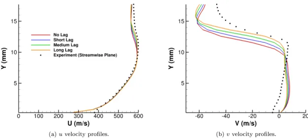
7.2 Particle Lag Eects
Velocity contours with the particle lag incorporated are shown in Fig. 38, with the remaining velocity contour plots located in appendix A. Note only the Standard and Combined cases are shown as they are representative of the spectrum of presented cases. Figures 39 through 42 showuandvvelocity proles with
and without particle lag at the most upstream axial location along with the rst intersecting spanwise data plane. See appendix B for remaining axial stations within the streamwise plane. The lag is shown to bring both the Standard and Combined cases closer to the experimental data with increasing lag time constant. Because the lag has such an eect, it is not advisable to use the workshop metric for comparing CFD to this PIV obtained experimental data without accounting for the lag. Recall that it is a fraction of the entire experimentally derived time constant that is used for the lag model. Although it is a very short time, it creates an error in the velocity eld that is higher than the desired match between the CFD and experiment.
Figure 38: v velocity streamwise contours for the experiment (top), short lag (middle-top), medium lag
(a)uvelocity proles. (b)vvelocity proles.
Figure 39: Select velocity proles at the most-upstream axial location (x= 18.191 mm) for the Standard
case.
(a)uvelocity proles (b)vvelocity proles
Figure 40: Select velocity proles at the rst intersecting spanwise plane (x= 20.76mm) for the Standard
(a)uvelocity proles. (b)vvelocity proles.
Figure 41: Select velocity proles at the most-upstream axial location (x= 18.191 mm) for the Combined
case.
(a)uvelocity proles. (b)vvelocity proles.
Figure 42: Select velocity proles at the rst intersecting spanwise plane (x= 20.76mm) for the Combined
case.
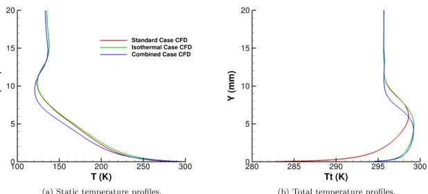
7.3 Isothermal Case
The eects of the Isothermal case can be seen in Figs. 43 and 44. Figure 43 and the static temperature prole in Fig. 44 show little dierence in the thermal boundary layer between the Standard and Isothermal cases. However, assuming the aluminum is isothermal is more realistic as there is likely heat transfer between the aluminum and the tunnel's surroundings. The temperature dierence is evident in the total temperature
center-span prole at the bottom wall, shown in Fig. 45. For reference, several notable stations have been marked to orient the prole. Figure 45 also conrms that the isothermal boundary conditions were implemented correctly and that the deviation from the constant total temperature for the Isothermal and Combined cases is due to the presence of the adiabatically modeled bottom window. Further, the isothermal boundary conditions were shown to have an eect on the total temperature prole, as shown in Fig. 44. The thermal recovery factor,rc, is determined to be 92.3% from the following equation:
Taw T∞ = 1 + rc 2 (γ−1)M 2 ∞ (95)
whereTawis the adiabatic wall temperature, or the total temperature evaluated from an adiabatic calculation.
This value ofrc is reasonable for turbulent ows as the recovery factor is approximately equal to the cube
root of the Prandtl number.
(a) Standard case CFD.
(b) Isothermal case CFD.
Figure 43: Freestream thermal boundary-layer atx=−63.9 mm. Temperature cut o is at 99% freestream
(a) Static temperature proles. (b) Total temperature proles.
Figure 44: Temperature proles at the most-upstream axial location (x= 18.191mm).
Figure 45: Total temperature centerspan prole at the bottom wall with the following stations marked: 1. Throat, 2. Trip location, 3. Start of the tunnel straight section, 4. Wedge leading edge, 5. Wedge trailing edge.
The dierences in temperature do correspond to dierences in velocity, as shown in Fig. 46. The Isothermal case is shown to be slightly worse than the Standard case as compared to the experimental data. The dierences in the velocities can be seen more clearly in the dierence contour plots shown in Figs. 47 and 48. The dierence is dened as the Isothermal case minus the Standard case. It is shown that the
interaction region for the Isothermal case is further upstream compared to the Standard case, and therefore further away compared to the experimental data. The movement of the interaction region is also veried in the static temperature dierence contour, shown in Fig. 49.
(a)uvelocity proles. (b)vvelocity proles.
Figure 46: Select velocity proles at the most-upstream axial location (x= 18.191mm).
(a) Positive dierence (m/s). (b) Negative dierence (m/s).
Figure 47: uvelocity dierence contours.
(a) Positive dierence (m/s). (b) Negative dierence (m/s).
(a) Positive dierence (K). (b) Negative dierence (K).
Figure 49: Static temperature dierence contours.
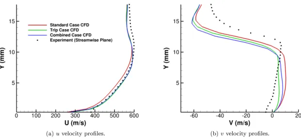
7.4 Trip Case
The eects of the Trip case are shown in Figs. 50 through 52. Figures 50 and 51 show that Trip and Combined cases agree well with the experimental data for theuvelocity which suggests that assuming the ow is laminar
at some portion upstream of the wedge is likely more correct than assuming it to be turbulent throughout. This further supports likely transition downstream of the throat based on the momentum thickness Reynolds number of the rst laminar case. The closeness of the uvelocity proles in Figs. 50 and 51 for the Trip
and Combined case indicates that the trip is a dominating factor that sets the Combined case apart from the Standard case. This is also evident in the turbulent kinetic energy proles shown in Fig. 52. Having a laminar region upstream of the wedge allows for thinner boundary layers, and thus less blockage, upstream of the wedge. This is further quantied by the throat blockage parameter, with the Trip case having a throat blockage of 1.11%, which is less than the 1.53% that it was for the Standard case.
(a)uvelocity proles. (b)vvelocity proles.
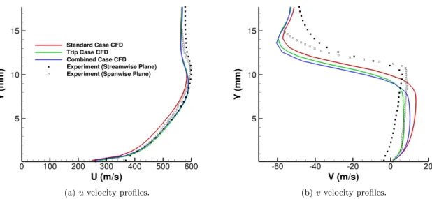
(a)uvelocity proles. (b)vvelocity proles.
Figure 51: Select velocity proles at the rst intersecting spanwise plane (x= 20.76mm).
(a) Atx= 18.191mm. (b) Atx= 20.76mm. Figure 52: Turbulent kinetic energy proles.
Examining the v velocity proles in Fig. 51 shows that the experimental data from the spanwise and
streamwise planes do not agree with each other. In fact, the CFD solutions are shown to match the experi-mental data from the spanwise plane better than compared to the streamwise plane. This is a key point when developing an error metric as the error metric used in the prior workshop focused solely on the experimental data in the streamwise plane and not the spanwise plane.
7.5 Turbulence Modeling Eects
Figures 53 and 54 show veloc