STRESS TESTING PROJECTED CAPITALIZED FARMLAND VALUES
A Thesis by BO GAO
Submitted to the Office of Graduate Studies of Texas A&M University
in partial fulfillment of the requirements for the degree of MASTER OF SCIENCE
Approved by:
Chair of Committee, John B. Penson, Jr. Committee Members, Danny A. Klinefelter
Sorin M. Sorescu Head of Department, C. Parr Rosson III
December 2012
Major Subject: Agricultural Economics
ii
ABSTRACT
This study initially presents historical trends in both the capitalized value and market value of farmland in the eight states comprising the Corn Belt and Lake States production regions as defined by the USDA. An econometric analysis of annual real cash rents per acre prior to determining the capitalized value of farmland in the eight states is then conducted. Two distributed lag models were hypothesized. The comparison of regression results of these two distributed lag models indicates that current year real cash rent can be best explained by current year real net farm income, lagged real net farm income over a period of years, and real cash rent in the previous year. A
spreadsheet simulation model is used to project capitalized farmland values in each state as well as regional averages over the 2012-2015 period. These projections reflect
alternative assumptions regarding future trends in real net farm income at the state level as well as the rate on 10-year constant maturity U.S. government bonds to assess the potential sensitivity of capitalized farmland values under adverse economic conditions. The projected trends in capitalized farmland values under two alternative stress
scenarios reflecting higher interest rates levels and lower net farm income levels indicates that capitalized farmland values are particularly sensitive to interest rate fluctuations since cash rent expectations of landlords are based on current and lagged historical profit performance.
iii
DEDICATION
There is no words can be found to exactly express my gratitude to my parents. I am dedicating this thesis to Heli Gao and Zhenhe Zhang, who gave me great support and their selfless love. I would not be who I am today without their love and encouragement.
iv
ACKNOWLEDGEMENTS
I would like to express my deepest gratitude to my committee chair, Dr. Penson. I do really appreciate his patience and guidance. I also would like to thank my
committee members, Dr. Klinefelter, and Dr. Sorescu. It is really a hard task to write a thesis. During this process, I learned not only the professional knowledge but also how to conduct a good research and be a qualified researcher. This thesis would not have
happened without their guidance, support and suggestion. This thesis has benefited from the joint efforts of my committee, especially my chair.
Thanks also go to my friends and colleagues and the department faculty and staff for making my time at Texas A&M University a great experience. I would like to thank Dr. Sorescu for giving me the opportunity to get a research assistant job to improve my research skill and overcome my financial difficulties at Texas A&M University. I would also like to present my gratitude to Dr. Bessler who gave me a lot of helpful suggestions. I also want to extend my gratitude to Mr. William Armstrong for his help on my research assistant job. I learned a lot form that experience.
v TABLE OF CONTENTS Page ABSTRACT ... ii DEDICATION ... iii ACKNOWLEDGEMENTS ... iv TABLE OF CONTENTS ... v
LIST OF FIGURES ... vii
LIST OF TABLES ... ix
CHAPTER I INTRODUCTION ... 1
Organization of Study ... 3
CHAPTER II LITERATURE REVIEW ... 4
Literature on Modeling Farmland Values ... 6
Literature on Modeling Capitalized Values ... 14
What is Missing in Literature? ... 17
CHAPTER III CAPITALIZED VALUE OF FARMLAND ... 19
Cash Rental Rate Component ... 19
Impact of Cash Rent on Farmland Prices ... 21
Interest Rate Component ... 22
Impact of Interest Rates on Farmland Prices ... 25
Quantifying Joint Impacts of Cash Rents and Interest Rates ... 29
CHAPTER IV MODEL DESIGN, DATA AND ESTIMATION ... 32
Scope of Analysis ... 32
Capitalized Values versus Market Value Trends ... 33
Econometric Analysis of Cash Rent ... 47
Data Series Used in Estimation ... 49
Econometric Estimation ... 51
vi
Page CHAPTER V STRESS TESTING FUTURE CAPITALIZED
FARMLAND VALUES ... 74
Spreadsheet Model of Capitalized Farmland Values ... 75
Projections of Capitalized Values under Alternative Scenarios ... 76
Implications for Producers and Lenders ... 93
CHAPTER VI SUMMARY AND CONCLUSION ... 95
Summary ... 95
Implications ... 97
REFERENCES ... 99
APPENDIX A ... 102
vii
LIST OF FIGURES
Page
Figure 1 U.S. Farmland Value 1950-2011 ... 7
Figure 2 10-year Constant-Maturity Treasury Bond Rate 1976-2011 ... 27
Figure 3 Farmland Market Values Versus Capitalized Values, Illinois, 1976-2011 ... 28
Figure 4 Farmland Market Values Versus Capitalized Values, Illinois, 1976-2011 ... 36
Figure 5 Farmland Market Values Versus Capitalized Values, Indiana, 1976-2011 ... 37
Figure 6 Farmland Market Values Versus Capitalized Values, Iowa, 1976-2011 ... 38
Figure 7 Farmland Market Values Versus Capitalized Values, Missouri, 1976-2011 ... 40
Figure 8 Farmland Market Values Versus Capitalized Values, Ohio, 1976-2011 ... 41
Figure 9 Farmland Market Values Versus Capitalized Values, Michigan, 1976-2011 ... 43
Figure 10 Farmland Market Values Versus Capitalized Values, Minnesota, 1976-2011 ... 44
Figure 11 Farmland Market Values Versus Capitalized Values, Wisconsin, 1976-2011 ... 46
Figure 12 Actual, Fitted, Residual Graph of Model2, Illinois ... 55
Figure 13 Actual, Fitted, Residual Graph of Model2, Indiana ... 57
Figure 14 Actual, Fitted, Residual Graph of Model2, Iowa ... 60
viii
Page
Figure 16 Actual, Fitted, Residual Graph of Model2, Ohio ... 65
Figure 17 Actual, Fitted, Residual Graph of Model2, Michigan ... 67
Figure 18 Actual, Fitted, Residual Graph of Model2, Minnesota ... 70
Figure 19 Actual, Fitted, Residual Graph of Model2, Wisconsin ... 72
Figure 20 Capitalized Values Under Different Scenarios, 2005-2015, Illinois ... 78
Figure 21 Capitalized Values Under Different Scenarios, 2005-2015, Indiana ... 80
Figure 22 Capitalized Values Under Different Scenarios, 2005-2015, Iowa ... 82
Figure 23 Capitalized Values Under Different Scenarios, 2005-2015, Missouri ... 83
Figure 24 Capitalized Values Under Different Scenarios, 2005-2015, Ohio ... 84
Figure 25 Capitalized Values Under Different Scenarios, 2005-2015, Michigan ... 86
Figure 26 Capitalized Values Under Different Scenarios, 2005-2015, Minnesota ... 87
Figure 27 Capitalized Values Under Different Scenarios, 2005-2015, Wisconsin ... 90
Figure 28 Capitalized Values Under Different Scenarios, 2005-2015, Corn Belt Region ... 91
Figure 29 Capitalized Values Under Different Scenarios, 2005-2015, Lake States Region ... 92
ix
LIST OF TABLES
Page
Table 1 Descriptive Statistics, 1950-2011 ... 52
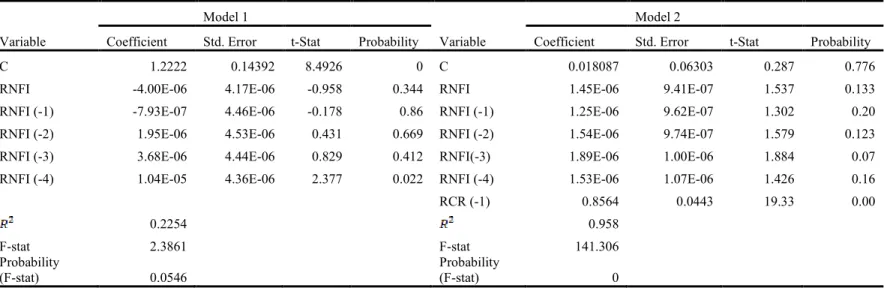
Table 2 Distributed Lag Model Estimation Results, Illinois, 1950-2011 ... 53
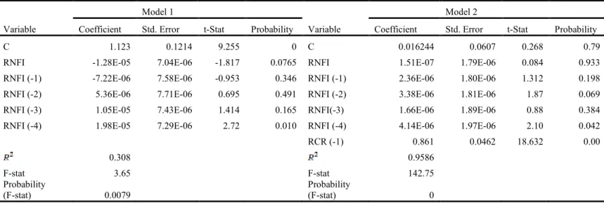
Table 3 Distributed Lag Model Estimation Results, Indiana, 1950-2011 ... 56
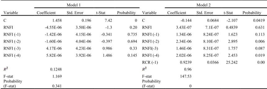
Table 4 Distributed Lag Model Estimation Results, Iowa, 1950-2011 ... 58
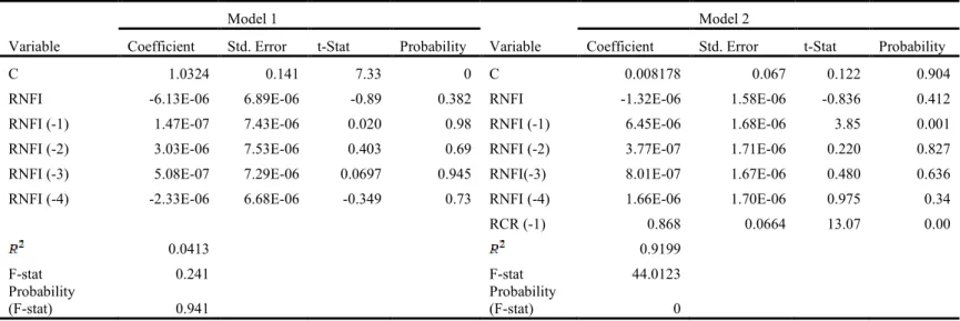
Table 5 Distributed Lag Model Estimation Results, Missouri, 1950-2011 ... 61
Table 6 Distributed Lag Model Estimation Results, Ohio, 1950-2011 ... 63
Table 7 Distributed Lag Model Estimation Results, Michigan, 1950-2011 ... 66
Table 8 Distributed Lag Model Estimation Results, Minnesota, 1950-2011 ... 68
Table 9 Distributed Lag Model Estimation Results, Wisconsin, 1950-2011 ... 71
1
CHAPTER I INTRODUCTION
Agriculture is an important industry in the U.S. economy, and is a major net exporter of raw agricultural products. The United States has a total land area of around 2.3 billion acres. There are 2.2 million farms in the U.S. covering an area of 922 million acres, which accounts for nearly 40% of the total land area in U.S. and represents an average size of 418 acres per farm (NASS, USDA 2012). Moreover, farmland is obviously a critical natural resource in the production of raw agricultural products. In addition, the financial well-being of owner-operators of farming operations can be heavily influenced by large fluctuations in farmland values because farm real estate represents the majority of assets on farm balance sheets and thus contributes heavily to their wealth position. Farmland values also affect the income and wealth position of non-operator landlords. Cash and cash equivalent rental rates affect the profitability of tenant operators. Finally, farmland values represent a source of security to agricultural lenders when making farm real estate mortgage loans.
The national farm sector balance sheet published by the U.S. Department of Agriculture indicates the sector is at an historic low leverage position largely because of rising farmland values. For example, the farm sector’s debt-to-asset ratio today is substantially lower than it was during the farm financial crisis in the early and mid-1980s, when farmland market values fell sharply. Thus, while farm debt nationally has risen in recent years to the levels observed in the 1980s, the sector’s leverage position
2
has fallen thanks to the rapidly rising farmland market values during the more recent biofuels era in agriculture. This is in spite of the major recession occurring in the U.S. economy during the 2007-2009 period. The uncertainty associated with these rapidly rising farmland market values has led some lenders to base their loan decisions on the capitalized value of farmland as opposed to its current market value. The sharp increase in farmland market values has led to concerns that the situation of the early-1980s, where sharp increases in farmland values were followed by sharp declines, could be repeated. That historical revaluation, along with recent annual double digit price increases, makes the issue of farmland valuation unprecedentedly popular.
The fact that farmland values account nearly 75 percent of the asset values on farm sector balance sheets has led to a considerable amount of research on the
determinants of fluctuations in farmland market values. Many studies on farmland market values have also focused on capitalized values, not only to show the historical trends of farmland and capitalized values, but also to explain the factors affecting trends in farmland market values. Although there have been numerous studies advancing alternative approaches to estimating farmland market values and capitalized farmland values, little has been done to project the future sensitivity to adverse economic
conditions, including the impact on farmland values of capitalization rate risk. Little has also been done to econometrically explain annual real cash rents per acre as a first step in calculating the capitalized value of farmland. In addition, stress testing of projected trend in capitalized farmland values under different adverse economic conditions is also missing in literature. This study will conduct an econometric analysis of annual real cash
3
rents per acre prior to projecting capitalized farmland values in two major agricultural regions in the U.S. over the 2012-2015 period.
Organization of Study
This study is organized as follows. Chapter II presents a review of the literature focusing on current market valuation and capitalized valuation with an emphasis on the methodologies used to explain these valuations. Chapter III introduces the approach taken in this study to modeling the capitalized value of farmland and projecting future trends in capitalized values under selected stress scenarios. Chapter IV will initially compare historical trends in both the capitalized and market value of farmland and then present the results from an econometric analysis of real cash rental rates for the
geographical locations targeted in this analysis. Chapter V describes the projections of future capitalized values under alternative stress scenarios for the 2012-2015 period. Finally, Chapter VI provides a summary and conclusions from this study.
4
CHAPTER II LITERATURE REVIEW
The literature is replete with analyses of U.S. farmland value trends and the determinants of fluctuations in these trends over time. The purpose of this chapter is to review the literature focusing on current market valuation and capitalized valuation with a focus on the methodologies used to explain these valuations.
Much of the equity of farmers who are owner-operators is associated with the market value of farmland. Changes in farmland values can affect their financial position as well as the value of collateral underpinning farm mortgages. Blank (2002) noted that ninety-five percent of the increase in farm equity during the 1998-2002 period was from increased equity in farm real estate. Ellinger (2011) noted that the leverage ratio would increase from 24 to 27 percent with a 30 percent decrease in farmland values. In addition, Calomiris, Hubbard and Stock (1986) noted that from 1980 to 1984, the average real value of U.S. farmland declined by almost 29 percent. The decrease was mainly pronounced in the Northern Plains and Corn Belt, which occurred during the period often referred to as the Farm Financial Crisis.For example, real farmland values in Nebraska fell to half of what it was in 1980. The erosion in the value of equity caused the leverage position of many farm borrowers to increase. The author also noted that delinquent loans had increased substantially, accounting for almost 7.5 percent of total loans at small agricultural banks by mid-1985.Farmland values have important effects on mortgage lending to farm borrowers.The loan-to-value ratio (LTV) is often used by
5
agricultural lenders when determining the maximum amount to lend. The LTV reflects the potential risk associated with the mortgage loan. The higher the LTV is, the higher the risk that the market value of the property will not cover the remaining balance on the loan. Since the property’s value is an important factor in understanding the riskiness of a mortgage loan, it is very important that agricultural lenders understand the dynamics of farmland value fluctuations. Koenig and Ryan (1991) noted in their paper that farmers had a strong demand for land during the 1970's and early 1980's. Farmers borrowed to expand their farms in part based on the expectation of potential capital gains associated with rapidly increasing farmland values along with low real interest rates. However, during the farm financial crisis of the 1980's, farmers' appetite for farmland and lenders' willingness to lend were dampened due to decreasing farmland values and mounting farm leverage positions.
The national farm sector balance sheet published by the US department of Agriculture today implies an all-time low farm leverage position in the farm sector due largely to rising farmland values. This aggregate picture of farm owner’s wealth position suggests the farm sector today is significantly less leveraged than it was in the early-1980s because today’s high farmland values. The uncertainty associated with these high farmland values has led many lenders to base their loan decisions on the capitalized value of farm property as opposed to its current market value. Barry, Hopkin, and Baker (1983) noted in their book that most potential buyers and sellers are not able to
determine actual values in the farm land market, so they hired appraisers who used the capitalization approach to find the appraised value. Due to the importance of the
6
appraisal function, many scholars conducted studies on factors affecting farmland values. However, recent years’ sharp increase in farmland values has led to concerns over a repeat of the situation of the early-1980s, where sharp increases in farmland values was followed by the largest price decline in modern history. That historical revaluation along with recent annual double digit price increases makes the issue of farmland values unprecedentedly popular. Shiller (2011) recently suggested that his favorite dark-horse candidate for an asset bubble this decade is farmland.
The balance of this chapter presents a review of the literature associated with various approaches to estimating farmland market values and capitalized values.
Literature on Modeling Farmland Values
From a long term perspective, U.S. national farm land values have trended upward but not with several periods of correction. Figure 1 shows the U.S. national trend in nominal farmland values from 1950 to 2011. From 1950 to the mid-1970s, nominal farmland values were relatively constant. During late-1970s and early-1980s, farmland values rose sharply. During the farm financial crisis of the mid-1980s, farmland prices decreased dramatically. Beginning in the late-1980s, farmland values have increased sharply with the exception of the 2007-2009 recession in the economy.
The farm sector has inherent characteristics of boom and bust asset value cycles not unlike other sectors of the economy. The dramatic appreciation of farmland values in the 1970s followed by the sharp correction in the 1980s is the most recent example of such a price fluctuation. The historical variation in farmland values attracts researchers
7 Resource: USDA available at http://www.nass.usda.gov/
8
to examine the economic factors determining these values and to assess whether farmland is overvalued or undervalued. Although the fundamental economic questions about farmland values have not changed, the approaches to estimating them have. This review provides a chronological account of the studies associated with various
approaches to estimating farmland values. Three main approaches have been used to estimate farmland values: (1) a reduced form-single equation econometric approach, (2) a structural econometric approach and (3) a time series econometric approach.
Reduced Form Single Equation Econometric Approach
Farmland value in Illinois and other Midwestern states have more than doubled since 1951. Until the early-1950's, the value of farmland was thought to be closely related to changes in farm commodity prices and net farm income. More recently farmland values have increased more than that suggested by the growth in net farm income. Klinefelter (1973) conducted a study attempting to identify the major variables affecting the farmland values in Illinois and to quantify the effect of these variables. His study was based on time-series data for the Illinois farmland market covering the period from 1951 to 1970. This time series was used to estimate the parameters of a single equation - reduced form model containing several the variables through to explain Illinois farmland values. The variables included the effect of inflation, government farm program payments, expected net rents, the number of voluntary transfers of farmland, farm enlargement, technological advance, and expected capital gains. The statistical results indicated problems created by multicollinearity in the single equation model. The
9
explanatory variables in his final equation included net rents, the number of voluntary transfers of farmland, average farm size, and expected capital gains. These variables were able to explain 97.3 percent of the changes in an index of Illinois real farmland values. After evaluating previous econometric models of U.S. farmland values using more recent data, Pope et al. (1979) found that single equation-reduced form model developed by Klinefelter had the best out-of-sample predictive performance. A paper by Scott (1983) focused on selected factors hypothesized to be most important in explaining the downward trend in farmland values during the period of financial stress in the early-1980s.
Scott argued that the expectations of future returns and values can affect the current farmland values significantly, finding that land prices began to increase rapidly after the commodity prices appeared to be permanently higher. Scott also noted that increasing inflation rate since the late-1960s was a factor influencing expectations, which in turn, affect farmland values. Finally, Scott suggested that the dramatic growth in real U.S. farmland prices in the 1970s can also be explained by the growth in real net farmland rental income.
Huang, Miller, Sherrick, and Gomez (2006) used a hedonic model to analyze Illinois farmland values that included such explanatory variables as land productivity, improvement, parcel size, the distance to urban areas, livestock production by farm density measures and swine operation scale, population density, income, and inflation. Their model’s fit was improved by the inclusion of spatial and serial correlation components. They concluded that farmland values increase with soil productivity,
10
personal income and population density, decrease with parcel size, distance to urban areas, and swine farm density.
As mentioned above, many researchers have examined the sensitivity of farmland values to returns to land, where cash rent is one measure of the return to farmland.
Structural Econometric Approach
A number of studies have used a structural econometric approach to analyzing factors affecting farmland values. Just and Miranowski (1993) developed a structural model of farmland prices which included the effect of changes in the opportunity cost of capital and the multidimensional impacts of inflation on savings-returns erosion, capital-erosion, and real debt reduction. They concluded that inflation and changes of the real returns on capital are the most important factors which explain changes in farmland values. They argued that these factors caused substantial appreciation in 1973, 1979, and 1982.
A study by Gertel and Atkinson (1993) compared the accuracy of forecasts of farmland values from a structural model estimated using ordinary least squares regression with forecasts using other techniques. They found that, given appropriate economic logic and data, forecasts from the structural model were preferred, particularly when the estimated model allowed for variable parameters.
11
Time Series Econometric Approach
Much of the previous literature in support of the present value method such as Burt (1986) used traditional time series regression analysis. Burt (1986) analyzed the dynamic behavior in farmland prices. Burt noted that there are two sources of dynamic behavior in the model, the expected rate of inflation and an exponential trend on rent expectations. But the expected rate of inflation and an exponential trend on rent
expectations did not have a significant effect on farmland prices. The dynamic structure of farmland prices can be quantified with time-series methods using data for a
homogenous area. The dynamic structure is captured by a second-order rational distributed lag on land rents using variables transformed to logarithms. Burt
approximated the composite effects of the adjustment mechanism for both farmland prices and expected rents with a multiplicative distributed lag specification on net rents. Burt assumed a constant real discount rate since investors were concerned with the long-run equilibrium rate and not annual changes in the real discount rate. Burt noted that the sum of two components can provide a good explanation for annual percentage changes in Illinois farmland prices. The two components are the percentage difference between the capitalized values of current expected land rents and the previous year expected farmland prices and the percentage change in expected farmland prices. However, Burt also noted that the percentage change in expected farmland prices was not the traditional measure of capital gains, but it was an exogenous measure based on a function of lagged rents. He concluded that land prices were impacted mostly by net rents changes and not by the speculative factors driving the values of non-income earning assets. The implicit
12
capitalization rate without tax on rents associated with equilibrium farmland price was 4 percent.
A study by Featherstone and Baker (1987) covered a much longer time frame. They used a vector auto-regression (VAR) that included equations for farmland values, returns to farmland, and interest rates. In each equation, lags of each variable were used as regressors. Results indicated that an oscillation in real asset values, real returns to assets, or real interest rates caused a process in which real asset values overreact. Although there will be an immediate reaction to a shock before the effect of the one-time, transitory shock begins to die out. Finally there will be an up to six years continued build-up in the asset value. This indicates a market with a propensity for an asset bubble. If irrelevant variables such as past capital gains rather than changes in returns and real interest rates were focused by market participants, such a bubble may arise. Their results indicated that speculative force is an important factor in determining farmland values in the U.S.
A different kind of empirical test of net present value based models of farmland prices appeared in the late-1980s and early-1990s with cointegration procedures and time series data. This approach can be used to deal effectively with two problems that exist in rational expectations present value models. One is the incomplete data about information of market participants. The other is nonstationarity of times series data. Campbell and Shiller (1987) found that, in their data set, the spread between long and short term interest rates seemed move closely with the unrestricted forecast of the present value of changes in the short run. It means that the deviations from the present
13
value model are temporary. In contrast, their evaluation of the present value model for stocks showed that the spread between stock prices and dividends moved very much and the deviations from the present value model are very persistent. Campbell and Schiller noted that if the present value model was correct, then net rents and land prices should have the consistent time series properties. Past values of the spread between land prices and land rents provides useful information in forecasting future changes in rents based on past changes in net rents. Campbell and Shiller found that short-term and long-term interest rates were consistent. They found that both savings and income included a single unit root.
Focusing on land rents and land values, Falk (1991) found consistency between land rents and land values for Iowa farmland, but he did not find them to be clearly cointegrated. In his paper, Falk did a formal test with Iowa farmland price and land rent data over the 1921-86 sample period. The results indicated that, although farmland price and rent movements highly correlated to each other, there was no consistency between price movements and the implications of this model.
Clark, Fulton and Scott (1993) examined relationships between farm income, land values, and capital asset pricing theory with two commonly referenced data sets, land prices and land rents. It is shown that land prices and land rents do not have the consistent time-series properties, a necessary condition for the simple capital asset pricing theory to hold. The differences between the farmland prices and land rents time-series data showed that farm income alone cannot explain the level of farmland values. Other factors may provide alternative explanations; this can be seen from historical data
14
that farmland prices increase and decrease faster than land rents. Clark, Fulton and Scott concluded that farmland prices do not perform consistent with many of the time-series representations used by former authors who tested land values data for explosive roots, which were not supported by the data they used. They noted that farmland prices appeared to have either one unit root or two unit roots. In addition, they also noted that the time-series representations of land prices and those of land rents were inconsistent, so referring that the simple asset pricing model did not hold. Clark, Fulton and Scott indicated there is a need for more complex models that allow for risk aversion, rational bubbles, and future changes in government policy or commodity prices. These
conclusions seem to be unique in the literature that examines the appropriateness of the capital asset pricing model during that period.
Literature on Modeling Capitalized Values
While many scholars conducted studies associated with alternative approaches to estimating farmland values, the others have focused on the estimation of capitalized values. . Two general approaches have been taken in the literature: a net present value approach and a capitalization of cash rent approach.
Net Present Value Approach
Shimoda and Jones (2011) described net present value models as a mainstream financial valuation tool that discounts an expected stream of future returns of an asset. Many scholars have used this approach to model capitalized values of farmland.
15
In a study on the magnitude and causes of asset appreciation done by Melichar (1979), he pointed that net farm income was inappropriate to be treat as a measure of the return to land. He noted that before farmland values are compared with net farm income, asset appreciation should be adjusted for general price inflation. As two comparable series, real unrealized capital gains are roughly equal to real net farm income. He also noted that over a 25-year period beginning in the mid-1950s, current returns to farm assets grew fast and that resulted in a low real rate of return to assets and large annual real capital gains. Based on this historical experience, Melichar took annual growth rate of farmland returns in to consideration to modify the capitalization formula.
The paper by Alston (1986) analyzed the two competing alternative explanations for the real growth of U.S. land prices: the real growth of rental income to farmland and the interaction of tax laws and inflation. He noted that real farmland prices growth can be explained mostly by real growth in net rental land income based on empirical analysis of U.S. and international farmland price data. The effect of inflation seemed to be
theoretically ambiguous. An increase in expected inflation had a negative effect of real farmland prices, but the impact of inflation has been relative small. Recall the present value model also formed the foundation of Burt’s study. However, in contrast to Burt, who assumed the capitalization rate constant, Alston allows for more flexibility in the capitalization rate. He also modified the capitalization formula because of the distinction between the tax rates.
16
Capitalizing Cash Rent Approach
The capitalization model emphasizes how farmland valuation develops. It is understandable that farmland values are typically based on the simple capitalization of rent model since more and more farmland is rented. The capitalization of rent valuation model simply equals the farmland cash rent divided by the capitalization rate. In recent years, many scholars used this approach to assess whether farmland was overvalued or undervalued. If farmland values are higher than the capitalized value, then farmland is said to be overvalued relative to its discounted future returns, and vice versa. Thus, this approach involves two key elements; cash rent and an appropriate interest rate.
Haugen and Aakre (2002) compared cropland values with a North Dakota farmland valuation model based on values generated by capitalizing the average cash rent for each county in that state.They found that annual cropland values for 2000-2002 as compared to values given by the rent capitalization method showed that the values given the land valuation model were higher. In addition, the results given by the land valuation model for pasture land was significantly different from the rent capitalization value of pasture in 2002, which does not exist in other analysis. They concluded that there was a significant difference in cropland values, and that a significant different did not exist for pasture land values.
Schnitkey (2010) mentioned that the decreasing farmland returns or increasing interest rates should happen before a large farmland price decline occurred. In addition, he noted that either could occur, but neither seemed likely in the near future. He also noted that in the next year, farmland returns seemed likely to increase because of above
17
average commodity prices, and interest rates increases seemed do not happen likely to change within the next year or two because the Federal Reserve seemed intent on implementing more quantitative easing. However, in long-run, he agrees with other authors’ opinion that farmland price will decline as interest rates rise.
Schnitkey and Sherrick (2011) analyzed whether farmland was at risk for a rapid and substantial decline. They noted this answer depended primarily on two factors: (1) the extent to which commodity prices have increased to new, sustainably higher levels which is caused by the increasing use of corn in producing ethanol and increasing demands for meat and grains in developing countries and (2) whether historically low capitalization rates continue to stay low into the future. They concluded that the two most likely factors to cause a price decline are declining commodity prices or increasing interest rates, and monetary and renewable fuel-based energy policy could be the triggers that cause farmland prices to fall. Nearly all recent studies have compared farmland market values and capitalized values to analyze farmland values.
What is Missing in Literature?
Although there are many studies advancing various approaches to estimating farmland values and capitalized land values, there is something largely missing in literature. Little focus has been given to an econometric analysis of annual real cash rent per acre as a prelude to determining capitalized farmland values. In addition, stress testing projected trends in capitalized farmland values under alternative adverse
18
economic conditions is also missing in literature. The approach taken in this study to address these underserved aspects of understanding farmland values is discussed in Chapter III
19
CHAPTER III
CAPITALIZED VALUE OF FARMLAND
The previous chapter presented a representative literature review of alternative viewpoints on the factors influencing historical trends in the market value of farmland. Relatively little attention has focused on capitalized farmland values. This chapter presents the approach taken in this study to modeling the capitalized value of farmland and the approach taken to projecting future trends in capitalized values under selected stress scenarios under alternative adverse economic conditions. Capitalizing the
expected cash rental income from leasing an asset based upon an appropriate interest rate is an approach frequently used to determine the capitalized value of an asset. The various factors that influence cash rental rates and the appropriate choice of a capitalization rate are initially addressed in this chapter.
Cash Rental Rate Component
The cash rental rate for a particular parcel of farmland is determined by the factors affecting the supply and demand for rented cropland in a specific location. Fundamental economic theory suggests that the supply and demand related factors determines the market equilibrium price. This holds true for cash rental rates, which represent the price for renting an acre of farmland. Theory suggests that if the supply of farmland available for rent increases, then the cash rental rate would fall. The opposite is true from a demand perspective; if the demand of rental farmland increases, cash rental
20
rates will increase. The equilibrium market cash rental rate reflects the price at which landlord and tenant expected rates of returns are relatively aligned.
Non-operator landlords make adjustments to their desired cash rental rates based, in part, on the expected profitability of the tenant’s farming operation. One of the major factors affecting cash rental rates is expected future net farm income.
Net Farm Income
Landlords make adjustments to the desired cash rental rate based on the expected profitability of the farmland leased to tenants. Net farm income is one measure of such profitability. Factors affecting expected net farm income include the quality of farmland reflected by normal yields per acre. Other factors include farm commodity prices and costs of production. Landlords make periodic adjustments to cash rental rates based not just one year but on the profitability of the farming operations over a period of several years. This can be seen as a distributed lag net farm income likely explains cash rental rate adjustments.
Other Factors
Other factors can influence cash rental rates, including landlord expected opportunity rates of return, location of the farmland, anticipated inflationary pressures and the existence of a surplus or shortage of farmland available for rent.
21
Impact of Cash Rent on Farmland Prices
Schnitkey (2010) suggests that cash rents represented the land owner’s return to farmland. Schnitkey and Sherrick (2011) focused on relative changes in cash rents and farmland prices in Illinois. They noted that, while both farmland prices and cash rents increased since 1987, farmland prices rose faster than cash rents as illustrated by
changes in cash rental as a percent of farmland prices. Decreasing cash rents as a percent of farmland price may suggest a future slowdown in farmland price trends. A trend that sees both farmland values and cash rents rising, but where cash rents grow at a slower rate, has also interested other researchers.
Ibendahl (2012), for example, examined the ratio of farmland values-to-cash rents determine if cash rents had changed in relation to farmland values. He noted the importance of this ratio as an indicator of whether cash rents were a good way of acquiring the use of farmland relative to purchasing farmland. He concluded that there might be a lag in cash rents before they match farmland prices level. However, this relationship does not always exist. Dobbins (2000), based on analysis of the data for Indiana, found that both farmland values and cash rents increased from 1999 levels, but that land values increased faster, causing cash rents as a percentage of land values to decrease. He focused on the value/rent multiple rather than the cash rent as a percentage of value.
Schnitkey also noted that, with regard to cash rents, there was considerable momentum for continued increases in cash rents in the future if the commodity prices, such as corn prices continue to increase. He noted that cash rents were a smaller
22
percentage of returns to farmland than occurring during the 2000 through 2005 period in most agricultural states. In addition, he argued that bidding among farmers for farm rental property can cause cash rental rate to increase unless commodity prices, such as corn prices, fall below normal price levels. Finally, Flanders, White and Escalante (2004) suggest that the determination of cash rents depends on expected farm returns, and because commodity prices are fluctuating and weather patterns are unpredictable, the residual “break-even” rent level can easily change.
Interest Rate Component
Another major component of the capitalized value approach is interest rates in general and the rate on long term U.S. Treasury bonds in particular. Thus it is important to also focus on the factors influencing interest rate fluctuations. There are a number of factors influencing interest rates. Some of the key factors are discussed in this section.
The Condition of the U.S. Economy
The changing economic condition of the U.S. economy can cause market interest rates to fluctuate. When the economy is growing, consumers have jobs and the demand for consumer durable and nondurable goods and services as well as housing expands. A portion of these expenditures are financed by credit extended from banks for large items, such as homes or cars, to finance these purchases. As the demand for credit increases, interest rates increase. Conversely, when the demand for credit decreases, interest rates may drop.
23
Inflationary Pressures
Inflationary pressures also play an important role in the interest rate changes. The rates on many loans are fixed in the loan contract. Lenders may be unwilling to lend money for a length of time if the purchasing power of money is expected to be less when the loan is repaid. Lenders will demand a higher interest rate known as an “inflation premium”. So inflation expectations may cause nominal interest rates to increase in an effort to gain the desired real interest income. Disinflation, on the other hand, may cause interest rates to decline.
Fiscal Policy Actions of the Federal Government
The federal government is the nation’s largest borrower. It has the highest credit rating, and the debt of federal government is treated as a preferred investment because of its taxing powers and the strength of the U.S. economy. Borrowing by the federal
government to finance its expenditures reduces the level of private credit available, which drives up interest rates in capital markets. This is often referred to as “crowing out”.
Federal farm commodity policy, to the extent that it stabilizes net farm incomes, also affects farmland values through capitalization of farm commodity policy benefits into farmland values.
24
Monetary Policy Actions of the Federal Government
The Federal Reserve System, the nation’s central bank, has key discretionary policy tools it can use to effect changes in market interest rates in normal times. Expansionary monetary policy actions taken to lower the federal funds rate will lower market interest rates and stimulate activity in the economy. Conversely, contractionary monetary policy actions to retard inflationary pressures will drive interest rates up and slow economic activity.
International Forces
International forces also can have a significant effect on interest rates. To extent that foreign investors are willing to lend their money to the U.S. by purchasing U.S. Treasury securities, interest rates will be lower than they would be otherwise. Potential contagion from global financial markets can also cause domestic financial markets to be more conservative in their lending policies, which can drive up interest rates to reflect a risk premium. An example is the current euro zone sovereign debt crisis and the
perceived risk and uncertainty associated with potential contagion to U.S. financial markets. Finally, should foreign purchases of government securities soften, the U.S. Treasury must pay higher rates on public borrowings to attract domestic investors, which can further increase crowding out in private markets and drive up interest rates.
25
Other Factors
Other factors can also cause interest rates to change. Changes in the relative health of the U.S. and global economies can lead to fluctuations in exchange rates which, in turn, can lead to policy changes that either directly or indirectly affect interest rates. Finally, meteorological and other unpredictable natural disasters may affect the demand of funds, which may also lead to interest rates change.
Impact of Interest Rates on Farmland Prices
There has been a great deal of focus on cash rents and returns to farmland when examining trends in farmland prices. Although these two factors deserve considerable focus, the impact that interest rate fluctuations play in influencing farmland prices should not be ignored. Interest rates not only influence the cost of borrowing to purchase farmland, but they also affect the opportunity rate of return on alternative uses of funds. In addition, the capitalized value of farmland is, by definition, directly affected by interest rates. Farmland prices and their capitalized value would be much lower had not interest rates decreased sharply in recent years.
Agricultural economists generally agree that farmland market values should largely reflect their discounted future returns, which includes both ordinary net income from operations as well as expected after-tax capital gains income. There are some models that incorporate spatial relationships of non-income benefits of ownership (Huang, et.al, 2006). Such non-pecuniary life style returns to ownership however are difficult to measure however. It is commonly agreed, however, that increases in returns
26
to farmland will causes farmland prices and capitalized values to increase while increases in the discount rate representing a long term interest rate would lead the decrease in these values.
Schnitkey and Sherrick (2011) focused on the use of the 10-year constant-maturity U.S. Treasury bond rate when discounting future returns to farmland. Figure 2 illustrated the historical trend in the 10-year constant maturity U.S. Treasury bond rate, which shows a break point in this trend. They noted that the nominal 10-year constant maturity U.S. Treasury bond rate has decreased since the early-1980s. Figure 2 highlights the decline in this time series from 13.91 percent in 1981 to a low of 2.79 percent in 2011. As interest rates decrease, capitalized asset values rise because future cash flows are discounted at a lower rate. The trend in farmland market values versus capitalized farmland values for Illinois is shown in Figure 3. Farmland is an infinitely-lived asset with a stream of expected net cash flows in perpetuity. Because of this feature, farmland prices are much more sensitive when interest rates change than other assets with a shorter useful life.
Schnitkey (2010) noted that decreasing interest rates counter decreases in cash rents relative to farmland prices. Falling interest rates tend to cause asset prices,
including farmland prices, to increase. Schnitkey advanced two reasons for this. First, it is typically easier to finance farmland purchases when interest rates are low. As interest rates decrease, borrowers pay less in loan payments, thereby allowing them to cash flow the financing of a larger parcel of land. Second, interest rates represent returns on alternative investment. As interest rates decrease, the attractiveness of alternative fixed
27
28
29
income investments drops relative to the investment in farmland, thereby making the purchase of farmland more attractive than if interest rates were high.
Recent minutes of the Board of Governors of the Federal Reserve System clearly indicate their intent to keep interest rates at current levels well into 2014. Thus the risk that rising interest rates would lower capitalized value of farmland is largely off the table. Any risk associated with declining farmland values therefore would appear to be tied to the factors affecting cash rental rates. This is a distinct possibility given the “flash” drought affecting the northern tier of states in 2012, where farmland values have been rising at double digit levels for five of the last six years according to published data (NASS). The extent of the drought effect will be mitigated by crop insurance indemnity payments and federal disaster programs.
Quantifying Joint Impacts of Cash Rents and Interest Rates
The capitalization formula for an infinitely-lived asset like farmland captures both the factors affecting landlord’s expected cash rental income and along terminterest rate. The long term interest rate serves as the capitalization or “cap” rate used to discount an expected stream of cash rents back to the present. The capitalization formula for an infinitely-lived asset can be expressed as follows:
CV = CRAC / CAPRATE where:
CV = capitalized value per acre
30 CAPRATE = the capitalization rate
The variable used to represent the capitalization rate (CAPRATE) is typically the 10-year constant maturity U.S. Treasury bond rate. This equation clearly suggests how a capitalized value would increase if interest rates decline or if cash rental income is expected to increase. If the capitalized value is greater than the existing market value, farmland is said to be undervalued. Conversely, if the capitalized value is less than existing market value, farmland is said to be overvalued. Figure 3 above, for example, showed that farmland values in Illinois were overvalued in the early-1980s. Subsequent corrections in the farmland market in the years to follow, when farmland values fell sharply, brought farmland values more closely into trend with capitalized values.
Schnitkey and Sherrick discussed this adjustment of farmland price occurring during the mid-1980s. They noted that, since 1986, farmland prices and capitalized values followed similar trends. On average, farmland prices were approximately 5 percent higher than capitalized values over the1986-2010 period. The rate of growth in both market and capitalized values between 2005 and 2010 rose sharply in many northern states because of the dramatic increase in energy-related commodity prices like corn and the sharp decline in interest rates.
While both market and capitalized values have risen sharply in recent years, farmland prices have not exceeded capitalized values to the degree observed in the 1980s. One can conclude that before farmland prices decrease, capitalized values probably have to fall, and capitalized values will decline if there is increase in interest rates or decrease in returns to farmland.
31
It is obvious that the decrease in interest rates in recent years has been a major factor in driving up capitalized values as well as market prices. This could lead to a major correction in farmland valuation, perhaps of the magnitude seen in the 1980s, should the U.S. economy recover faster than currently expected, which could lead to higher interest rates.
32
CHAPTER IV
MODEL DESIGN, DATA AND ESTIMATION
The national farm sector balance sheet published by the U.S. Department of Agriculture implies an all-time low aggregate farm leverage position due largely to rising farmland values. It is true that the farm sector is significantly less leveraged than it was back in the early-1980s. The level of farm debt outstanding has increased much more slowly since the mid-1980s than the value of farmland. Many lenders, in times of uncertainty, may tend to base their mortgage lending decisions more on the capitalized value of farmland as opposed to its current market value.
One of the stated objectives of this study presented in Chapter I was to stress test projected trends in the capitalized value of farmland in selected key agricultural
production regions where market values have been increasing at double-digit rates. To achieve this objective, this chapter study will initially compare examine historical trends in both the capitalized and market value of farmland. The results from an econometric analysis of real cash rental rates for these locations targeted will then be presented. Projections of future capitalized values under alternative stress scenarios for the 2012-2014 period based on these econometric results will be presented in Chapter V.
Scope of Analysis
There are ten farm production regions in the U.S. according to the U.S.
33
Plains, Lake States, Corn Belt, Delta States, Northeast, Southeast and Appalachian regions. This study focuses on two of the Corn Belt and Lake States regions where major farm commodities play an important role in state revenue and where farmland prices has risen at double digits rates in recent years.
One of the major factors influencing farmland values in these two regions is the direct effect that renewable fuel mandates have had on corn prices and the indirect effects on other major commodities. In the following sections, the historical trends in farmland market values and capitalized values for the eight states comprising these two regions are presented. These states are Illinois, Iowa, Indiana, Michigan, Minnesota, Missouri, Ohio and Wisconsin. In addition, the econometric approach used in this study to model real cash rent per acre is presented, followed by a discussion of the estimated equations. The capitalized values will then be determined by dividing projected cash rents by the 10-year constant maturity Treasury bond rate.
Capitalized Value versus Market Value Trends
Based on the approach introduced in Chapter III, the historical capitalized value of farmland in these two production regions was calculated. The calculated capitalized values are then compared to the historical market values in each of these eight states. The following graphs show how farmland market values versus capitalized values have changed over the 1967-2011 period.
34
Corn Belt Region
The Corn Belt production region consists of the following states: Illinois,
Indiana, Iowa, Missouri and Ohio. The trends in market and capitalized farmland values are described in these states below.
The capitalized values provided by the capitalization equation discussed in Chapter III closely follow farmland market values in Illinois as can be seen in Figure 4. The only major divergence between farmland market values and capitalized values happened during the early and mid-1980s. The largest divergence occurred in 1981; the farmland market of $2,188 per acre was 1.67 times the capitalized value of $818 per acre. From1981 to 1986, farmland market values fell from $2,188 per acre to $1,232 per acre, which was actually a little below the capitalized value of $1,301 per acre. Since 1986, farm land market values and capitalized values have tracked each other closely, with market values running approximately 5 percent higher than capitalized values on average from 1986 through 2011. Because of the increase in commodity prices in general and corn in particular, Illinois farmland prices increased from $3,210 per acre in 2005 up to $5,700 per acre in 2011, an increase of 77.6 percent. During the same period, capitalized values actually increased at a faster rate. In 2011, capitalized value of $6,559 per acre were actually larger than the market value of $5,700 per acre, suggesting that farmland in 2011 was somewhat undervalued based on its capitalized value While net farm incomes in Illinois have risen over the period, leading to higher cash rents, the 10-year constant maturity Treasury bond rate has fallen sharply. This added to the rising capitalized value based on profitability.
35
The capitalized values and current market values also track each other closely as can be seen in Figure 5. Like Illinois, the most recent major divergence between market values and capitalized values in Indiana happened during the early and mid-1980s. The largest divergence occurred in 1981 where the market of $2,031 per acre was 1.61 times the capitalized value of $779 per acre. Between1981 to 1986, market values in Indiana fell from $2,031 per acre to $1,167 per acre, which was very close to the capitalized value of $1,115 per acre. Since 1986, farm land market values and capitalized values have also tracked each other closely in Indiana. But market values were nearly 21 percent higher than capitalized values on average from 1986 through 2011. Market values increased from $3,000 per acre in 2005 to $4,800 per acre in 2011, an increase of 60 percent. Capitalized values increased at an even faster rate. The capitalized value of $5,448 per acre in Indiana was higher than the market of $4,800 per acre in 2011. This suggests that Indiana farmland was undervalued from a capitalization perspective last year.
In Iowa, the capitalized values closely follow farmland market values, as can be seen in Figure 6. A major divergence between the market value and capitalized value happened during the early and mid-1980s, much like Illinois and Indiana. The largest divergence occurred in 1981; the farmland market of $1,999 per acre was 2.45 times the capitalized value of $817 per acre. From1981 to 1986, Iowa farmland market values fell from $1,999 per acre to $873 per acre, which was below the capitalized value of $1,141 per acre. Since 1986, the trend in market values and capitalized values in Iowa have tracked each other closely, although market values were nearly 2.6 percent below
36
37
38
39
capitalized values on average from 1986 through 2011. An average market value of $5,600 per acre in 2011 was 112 percent higher than the average of $2,640 in 2005. However, capitalized values increased at an even faster rate. By 2011, the capitalized value of $7,025 per acre was substantially higher than the market value $5,600 per acre, again suggesting the Iowa farmland was undervalued from a capitalization perspective last year.
The capitalized value of farmland in Missouri closely follows market values as illustrated in Figure 7. Much like the other Corn Belt states, the capitalized value dipped below market values during the farm financial crisis. The largest divergence occurred in 1981 where the market value of $990 per acre was 2 times the capitalized value of $495 per acre. Since that major correction, market values have closely tracked their
capitalized values until the last few years where a sharp decline in interest rates helps explain a sharp increase in the capitalized value In 2011, the capitalized value of $3,799 per acre was larger than the farmland price of $2,530 per acre, suggesting at current rates farmland in Minnesota was undervalued from a capitalization perspective.
The capitalized values of farmland in Ohio exhibit an upward trend over the 1976-2011 period as do market values (Figure 8). The major divergence between market values and capitalized values again occurred during the farm financial during the early and mid-1980s. From1981 to 1986, market values in Ohio fell from $1,831 per acre to $1,136 per acre, which was still higher the capitalized value of $915 per acre. Since 1986, market values in Ohio were above capitalized values. But this gap closed in 2011, when the capitalized value of $3,943 per acre was 8 percent lower than the farmland
40
Resource: USDA available at http://www.nass.usda.gov/, Federal Reserve Economic Data available at http://research.stlouisfed.org/fred2 Note: data from 1995-2008 is not available.
41
42
price of $4,300 per acre suggesting a slight overvaluation of farmland from a capitalization perspective.
Lake States Region
The Lake States production region consists of the following states: Michigan, Minnesota and Wisconsin. The trends in market and capitalized farmland values are described in these states below.
While both capitalized values and market values have exhibited an upward trend over the 1976-2011 period in Michigan, the divergence has been greater than observed in the Corn Belt states of Illinois, Indiana and Iowa (Figure 9). Michigan has a greater commitment to the dairy industry, which has suffered relatively lower profit margins than these more heavily corn-based states. This helps explain the much lower capitalized values relative to market value. From1981 to 1986, market values fell from $1,289 per acre to $1,012 per acre. Since 1986, both market values and capitalized values have risen. Market values rose by 25 percent from $3,070 per acre in 2005 to $3,850 per acre in 2011, a slower rate than seen in the Corn Belt states of Illinois, Indiana and Iowa. In 2011, capitalized value of $3,226 per acre was below the market value of $3,850 per acre, which suggests that farmland is overvalued in Michigan from a capitalization perspective. The capitalized values track market values closely in Minnesota as shown in Figure 10. A major divergence between market values and capitalized values occurred during the farm financial crisis during the early and mid-1980s. The largest divergence occurred in 1981 where the average market of $1,281 per acre was 2.59 times of the capitalized value of
43
44
45
$495 per acre. During the1981-1986 period, market values fell from $1,281 per acre to $694 per acre, which was little below the capitalized value of $701 per acre. Since 1986, market values and capitalized values have tracked each other closely until the last few years when market values rose sharply reflecting higher grain prices. Market values in 2011 averaged $3,350 per acre, an increase of 63 percent over 2005 market values. During the same period, capitalized values increased at an ever faster rate than market values. In 2011, the capitalized value of $4,839 per acre was much higher than the farmland price of $3,350 per acre. This suggests that farmland in Minnesota was undervalued from a capitalization perspective.
The capitalized value and market value of farmland in Wisconsin also exhibits an upward trend over the 1976-2011 period as shown in Figure 11. Like the other states, the capitalized value fell sharply below the market value during the farm financial crisis in the early and mid-1980s. From1981 to 1986, farmland market values fell from $1,152 per acre to $836 per acre, which was higher than the capitalized value of $635 per acre. Since 1986, farm land market values were increasingly well above the corresponding
capitalized values. This is despite capitalized values rising at a faster rate over the 1986-2011 period. In 1986-2011, the capitalized value of $3,548 per acre was lower than the market value of $4,050 per acre, suggesting that farmland is overvalued from a capitalization perspective.
From above graphs and description, it is clear how market values and capitalized values of farmland change in past. Thecapitalized value of farmland may be used by many lenders in time of rising risk when making loan decisions. Projecting capitalized
46
47
values over 2012 to 2014, which will be important from both an ownership as well as a lenders perspective is an important aspect of this study. To project capitalized value, the first step is to econometrically project future trends in annual cash rent per acre.
Econometric Analysis of Cash Rent
As discussed in Chapter II, non-operator landlords make adjustments to their desired cash rental rates based in part, on the expected profitability of the tenant’s farming operation. Net farm income represents a measure of profitability. Thus,
expected future real net farm income can considered as a major factor affecting real cash rental rates.
To assess the effect of the real net farm income on real cash rent, this study will use a distributed lag model to capture this effect. Non-operator landlords make
adjustments to their desired cash rental rates based on the expected profitability of their tenants. Moreover, when considering the fluctuation in annual net farm income,
landlords base their expectations, in part, upon net farm income in previous years. A distributed lag model is one approach used to predict current values of a dependent variable based on both the current values and the lagged values of an explanatory variable. The distributed lag model has used in many time series data studies. Lambert and Griffin (2004) used a distributed lag model to examine factors as commodity prices, soil productivity and government payments on cash rental rates. A distributed lag model was also used by Fouda (2010) to analyze the inter-temporal impacts of selected
48
investment had a positive effect on Cameroonian growth in the current year, government expenditures had a negative effect after one year.
As is mentioned above, this study selects a distributed lag model as the
appropriate approach to quantify current and past real net farm income on real cash rent. The general form of the distributed lagmodel used in this study to project real cash rent per acre is given by:
where:
RCR real cash rent given by cash rent per acre divide the GDP deflator.
RNFI real net farm income given by net farm income divided the GDP deflator. The expected sign for the coefficients on the current and lagged real net farm income should be positive because the non-operator landlord is hypothesized to adjust cash rental rates based on the weighted current and lagged profitability of the leased land. As net farm income increases, non-operator landlords will charge more rent.
This study also examined the effect of adding the lagged dependent variable on the right-hand side of the previous equation to further examine the speed of response to current and lagged real net farm income. The expected sign for the coefficient on the lagged dependent variable should also be positive. This second model would take the following form:
49
Data Series Used in Estimation
The definition of the variables used in this study and the sources of data used in this study are described in this section.
Net Farm Income
Net farm income reflects both monetary and non-monetary returns to farm operators after all production expenses have been deducted. Gross farm income includes cash receipts, the value of home consumption of farm production, the imputed value of the farm dwelling and the net inventory change. Farm production expenses captures cash expenses, which includes hired labor costs, interest and property taxes, plus depreciation of machinery, equipment and buildings. The data for net farm income used in this study was collected from the Economic Research Service, U.S. Department of Agriculture over the 1950-2011 period at the state level. The states are the eight states comprising the Corn Belt and Lake States regions mentioned above.
10-year Constant Maturity Treasury Bond Rate
The 10-year constant maturity U.S. Treasury bond rate published by the Board of Governors of the Federal Reserve System is the interest rate the federal government would pay the bondholder for every 10 years. From the daily yield curve, which relates the yield on a security to its time to maturity, the U.S. Treasury determines yields on Treasury securities at a constant maturity for a variety of terms or maturities. The data over 1950-2011 periods of 10-year constant maturity Treasury bond rate was used as the “capitalization rate” to calculate the capitalized values in this study.
50
Cash Rent
Cash rent refers to the amount of money paid as rent to the non-operator landlord. While not examined in this study, share rents could be converted to a cash equivalents basis. Annual data for cash rent over 1950-2011 period for each of the eight states was obtained from the National Agricultural Statistics Service, U.S. Department of Agriculture.
Farmland Value
The historical farmland values presented in this study represent the value of crop and pasture land, and exclude buildings and other capital improvements. The data series are published by the National Agricultural Statistics Service, U.S. Department of
Agriculture. The data series covers the 1950-2011 period for the eight states comprising the Corn Belt and Lake States regions.
GDP Deflator
The price deflator for gross domestic product (GDP) is commonly referred to as the implicit GDP price deflator. It is an index of the level of prices of all goods and services in the U.S. economy.This index is used to measurereal GDP. The time series for the implicit GDP price deflator is published by the Board of Governors of the Federal Reserve System. The data series used in this study covers the 1950-2011 period, and is
51
used to measure the real cash rents and net farm income to account for the influence of inflation.
A statistical description of the variables used in this study is presented in table 1 below.
Econometric Estimation
This section describes the econometric results from estimating the impact of real net farm income on real cash rent. The Eviews 6.0 econometric package was used in this study to estimate the coefficients in the two real cash rent distributed lag models in presented in Chapter III. The application of regression analysis will quantify whether or not the coefficients on the independent variables are statistically significant and the impact that current and lagged variables have on explaining real cash rent per acre in each state. The details from this regression analysis are presented in the following tables. Notable highlights in these estimated equations are discussed as well.
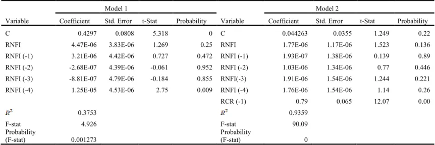
Table 2 compares the regression results for model 1 and model 2 for real cash rents in Illinois. The signs on several coefficients in for model 1 are different than expected; the coefficient on current real net farm income and real net farm income lagged one year are negative rather than positive. The signs on all real net farm income variables have the expected signs in model 2. In addition, the coefficient on the lagged dependent variable adds to the explanation of the speed to which non-operator landlords adjust real cash rents. Overall, model 2 outperforms model 1; the student t test statistics
52
Table 1- Descriptive Statistics, 1950-2011
Variable Mean Standard Deviation Min Max Variable Mean Standard Deviation Min Max
GDPDEF 53.4310 32.84725 14.648 113.357 10YCTBR 6.286 2.688 2.4 13.91 NFI Iowa 1893990 1411649 -68864 7025965 CR Ohio 63.846 26.633 4.98 110 NFI Illinois 1386074 987949.9 -488113 5333209 CR Wisconsin 49.33 21.957 5.82 99 NFI Indiana 794492.7 627938 -385635 3172417 CR Illinois 94.93 41.963 9.07 183 NFI Michigan 532344 391681 218496.2 2033040 CR Michigan 45.68 20.44 3.97 90 NFI Minnesota 1286562 1071144 86338.1 5836394.9 CR Indiana 82.91 34.98 6.83 152 NFI Missouri 822048.6 640913 62824 3055181 CR Minnesota 60.44 29.99 4.88 135 NFI Ohio 800586.7 531452.6 -43668 2246961.9 CR Missouri 50.05 26.1 3.19 106 NFI Wisconsin 944947.7 547878.8 318594.9 2577221 CR Iowa 95.62 43.63 8.51 196 MV Wisconsin 1015.41 1091.043 89 4050 MV Illinois 1488.3 1292.3 174 5700 MV Ohio 1339.43 1159.238 136 4300 MV Missouri 732.1 660.4 64 2530 MV Michigan 1159.62 1116.968 99 3900 MV Indiana 1354.98 1178.3 137 480