Stock Market Returns Predictability:
Does Volatility Matter?
Chao Sun
Feb, 2008
QMSS Master Thesis, Columbia University
Advisor: Christopher Weiss, QMSS, Columbia University
Stock Market Returns Predictability: Does Volatility Matter?
Chao Sun
The article examines whether the stock market is predictable, and provides evidence that several basic financial and economic factors have predictive power for the market excess return. The model built with such factors is good for in-sample predictability, but has poor performance for out-of-sample predictability. We find the variable of unexpected market volatility added in the model can greatly improve the out-of-sample predicting ability for excess return. Such improvement is significant, but the forecasting model might still needs some other explanatory variables to be included.
Section I: Introduction
The debate about whether the stock returns can be predicted has always been a hot arguable issue in the financial studies of asset pricing. Although some authors, such as Lo and MacKinnlay (1990), point out that the models for predicting the stock returns might be just data snooping, it is still widely believed that some financial and economic factors can explain much of the variation of the stock returns so as to have a great forecast power for stock return. Take, for example, the articles by Keim and Stambaugy (1986), Fama and French (1988), Campbell and Shiller (1988), Ferson and Harvey (1991, 1993), Whitelaw (1994), Pesaran and Timmermann (1995), Pointiff and Schall (1998) Bossaerts and Hillion (1999) and Martijn Cremers (2002). In these papers, the stock returns are suggested to be predictable by a linear model with some financial predictors such as earnings yield and some economic cycle components as
well, including interest rate1, inflation rate, industrial production growth and etc.
One argument about stock return predictability is that if the stock return could be predicted, then everybody would go for the predictable profit and therefore such good opportunity might soon vanish even before the investors build their models. However, there are still a lot of financial institutions and even some individuals following this method. Two explanations can help us to understand the popularity of predicting models. Some of the investors2 believe that the profitable chance can never be exploited, because some models might be overlooked or undiscovered yet by other investors due to lack of time, knowledge or resources. It costs a lot to cover the expenses associated with analyzing the data and finding the forecasting models, so the investors must have an incentive to spend so much. To some extent, the popularity of the stock return forecasting models itself proves that the stock returns can be predicted and can be used to generate higher investment profits for the person who discovers the model. Another explanation is that the power of predictors change over time, so the best prediction model would not always stay the same and the predictable profit opportunity would appear again. Pesaran and Timmermann (1995) indirectly provide some evidence for this thought, as they find out that prediction performance improves if the forecasting models are adjusted over time.
The basic theory for the stock return forecasting is the capital asset pricing model (CAPM)3 which suggests that the excess stock returns is related the systematic risk of the market. The market risk is reflected in the variation of market returns which is
1 Breen, Glosten and Jagannathan present some persuasive results which suggest that the nominal interest rates
are of great importance to forecast nominal return on stocks. (Economic Significance of Predictable Variations in Stock Index Returns, 1989)
2 The investors in this paper refer to both the individuals and financial institutions those are holding positions in
the stock market.
3 The prominent capital asset pricing model (CAPM) introduced by Sharpe (1964) and Lintner (1965) is
believed to be fundamentally decided by the macroeconomic factors such as yield and term spread in the corporate bond and government bond markets. The explanatory power of these factors have been verified by some researchers4, so it leads to the conclusion that significant variation in excess returns over the economic cycle can be predicted by these macroeconomic factors.
Besides, the time series theory gives us some insights into the serial correlation effect5 over time of the financial data, and it also provides some methods to account for it. Using lots of financial time series data, the stock return predicting model should also take the serial correlation problem into account. Prior empirical studies shows that several most recent lagged returns might have some mixed correlation and such sophisticated autocorrelation makes the variables of lagged excess returns crucial in the predicting model. Martijn Cremers (2002) summarizes that most of the models in previous research take the lagged returns into account6, and his model is not an exception. Referring to the number of lags included, there is no agreement reached, but a quite small number would be preferred to avoid data snooping problem. Another concern about it is that some of the time variation in stock return could probably explained by the other economic cycle components as what we have mentioned already, and therefore no need to include too many lagged returns.
This article also adopts the traditional method of linear regression to figure out the predicting model for the whole US financial market, if it does exist. The composite equity indices are the only targets aimed at in this paper, because not only they are
4 For example, Chen, Roll and Ross (1986) includes credit spread in corporate bond market, term spread and yield
spread in government bond market in their model. Ferson (1990) uses the following variables in his model: Treasury Bill yield, change in Treasury Bill yield and yield spread in government bond market.
5 Serial correlation is the correlation of a variable with itself over successive time intervals. Such effect often
occurs when the data are collected over time and the observations got close together are related with each other, which is always the case with financial data. (The Statistical Sleuth by Ramsey and Schafer, 2002)
good proxies of the entire financial market, but also they are more closely related to the macroeconomic changes. In fact, the market premium/excess return, with the β
factor, is also the key factor to decide the other stock excess returns according to the theory of CAPM. In this way, if we can predict the market excess return, then we can predict other stock returns with the β estimated. In our model, we will try to take two lagged excess returns, some profitability variables for the index, several major economic variables and other influential predictors into account. Besides the potential variables, the interaction terms and polynomial forms are also checked, according to the recent finding by Abhyankar, Copeland and Wong (1997) that nonlinear dynamics exist between the financial and economic variables. However, not all of the variables are part of the final forecasting model, since different variable selection methods7 are tried and only the ones with favorable fitting results and good predictability are chose.
Before reaching the predicting model, two issues probably impede us from drawing conclusions. One is the model overfitting problem (a.k.a. “data snooping”) discovered by Lo and MacKinlay (1990). The other is the poor out-of-sample performance that has long been talked about. Goyal and Welch (2006) conducted a comprehensive examination of the existing evidence, and show that stock returns are hardly predictable in the out-of-sample context. Almost all the theoretical interpretation of excess return predictability is inevitably based on the model obtained, so the two problems could be fatal to the predicting models, nevertheless it is worth trying. In fact, many methods have been used to solve the problems. For instance, Akaike’s information criterion8 might be the most well-known model selection criteria used to
7 The potential variable selection methods include Stepwise Regression, Lasso Method, All Subset Method,
10-Fold Cross Validation, Zheng-Loh Method, and Forward Stagewise Regression.
8 Akaike's Information Criterion is a criterion for selecting among nested econometric models. The AIC is a
number associated with each model: AIC=ln (Sm^2) + 2m/T, where m is the number of parameters in the model, and Sm^2 is the estimated residual variance in an AR(m) example: Sm^2 = (sum of squared residuals for model m)/T. That is, the average squared residual for model m.
guard against overfitting, and other formal model selection criteria9 would work as well. To improve the out-of-sample predictive accuracy, some efforts have been put into finding alternative forecasting strategies to linear specifications, such as what have done by Lewellen (2004), and Lettau and Nieuwerburgh (2006). Qi and Maddala (1999) also demonstrate the method of neural networks which can model flexible linear or non-linear relationship and get better predicting ability. However, there is no widely accepted method to get out of the trouble of poor out-of-sample predictability.
In this paper, we try to add a volatility expectation factor in the model, and see whether this would help get better models with the predictive power. The thought was inspired by the fact that the expected market volatility can greatly influence the investor behavior so as to stabilize or magnify the effects of other variables’ change. In such a way, volatility expectation plays an important part in forecast the market excess return. Unexpected volatility10 should also be considered in the model, even if it contributes little to the forecasting part.11 Considering the possible values for the unexpected volatility into prediction, a range for predicted excess return is returned which can be quite useful.
The other parts of the article are organized as follows: Section II discusses about explanatory variables included in the model and describes the data set we use; Section III introduces all the model selection criteria adopted and compares the raw results from them; Section IV gives out the model obtained without the volatility expectation
8 The criterion may be minimized over choices of m to form a tradeoff between the fit of the model (which
lowers the sum of squared residuals) and the model's complexity, which is measured by m. Thus an AR(m) model versus an AR(m+1) can be compared by this criterion for a given batch of data.
An equivalent formulation is this one: AIC=T ln(RSS) + 2K where K is the number of regressors, T is the number of obserations, and RSS is the residual sum of squares; minimize over K to pick K.
9 Bayesian model selection framework also works well for limiting data snooping.
10 The unexpected volatility is calculated as expected volatility for the current period minus the realized volatility
for the past period.
factors, and check the predictive power of it; Section V includes the expected and unexpected volatility and does the model selection again to see how the predicting ability could be improved; Section VI provides a summary of the main findings and tries to make a conclusion.
Section II: Variables and Data Set
In order to predict the U.S. stock market excess return, a proxy variable for this response variable has to be decided before moving onto the discussion about the explanatory variables. The indices Standard & Poor 50012(S&P 500) and Russell 100013are both good choices as the benchmark of the entire stock market. Basically, S&P 500 is the main part of our analysis, and Russell 1000 is employed as a model “double check”. For the explanatory variables, quite a number of financial and economic variables have shown some predictive power for the market excess return, and they provide the starting point for the empirical interpretation that follows. Therefore we include all the potential predictors, and generally, the variables could be categorized into seven groups - technical, profitability, liquidity, volatility, interest rate, inflation rate and real output variables.14
The technical variables mainly refer to the market excess returns including lagged excess returns. As the autocorrelation of the stock return is widely believe to persist in financial data, such time serial correlation effect must be accounted for in the model.
12 S&P 500 Index is a market-value-weighted equity index consisting of 500 stocks chosen based on their market
size, liquidity and industry grouping and some other factors. Stocks included in the index are selected by the S&P Index Committee, a team of financial analysts and economists at Standard & Poor's.
13 Russell 1000 Index is a market-capitalization-weighted equity index maintained by the Russell Investment
Group. More specifically, this index encompasses the 1,000 largest U.S.-traded stocks, in which the underlying companies are all incorporated in the U.S..
14 The first four groups are index-related financial variables, and the other three groups are macroeconomic-
Considering the number of lags included, most of the researchers believe that two lag returns should be enough, because much of the time-variation of excess returns is explained by other variables rather than itself. In our model, two also test the first two lag excess returns, although the test result from autocorrelation function shows that only one lag autocorrelation is significant (Figure One). Besides, January dummy variable is also a necessary technical variable, as the “January effect”15 is believed to possibly affect the stock market in some way.
Figure One: Autocorrelation for Excess Return16
0 5 10 15 20 25 0. 0 0. 4 0 .8 Lag AC F Series Excess_Return_SP500
The profitability variables for chose composite indices include earnings yield and dividend yield. Obviously, earnings yield represents the growth opportunity which would guide the market’s expectation of the future excess return. Ang and Bekaert (2006) test the predictive power of dividend yield for forecasting future excess returns especially at short horizon.
The liquidity of the market is measured by the variable index traded volume over price level. A more liquid market is believed to be the reflection of faith in the market, and might promise a better future return of the market. Actually, the volume over
15 “The ‘January effect’ has been used to refer to the phenomenon in which small-cap securities often have had
higher rates of return in past Januarys [1979-2005]”. (from official website of Chicago Board Options Exchange)
price variable is a poor proxy for the liquidity, as the correlation between them is not linear or even not monotonic. However, some attempts still will be taken out, aiming at figuring out the complicated correlation between the future excess return and the liquidity variable.
The last group of variables related to the indices is volatility expectation variable which are used for extensive predicting model. The natural choice of such variables would be the volatility index17 tracking the market index, because they directly measure the volatility expectation. The unexpected volatility is also added in the extensive model, and it is calculated as the difference between the actual volatility and the expected volatility over the same time period.18
The first group of macroeconomic variables are the interest rate related factors, including the interest rates of both the corporate bond market and the government bond market: credit spread between the yields of investment grade (Moody’s AAA19) and below Investment grade (Moody’s BAA20) bonds, yield on a short-term Treasury bill21 (3-month Government Bond), term spread22 between the short-term Treasury bill yield and the long-term government bond(10-year Government Bond) yield, and yield spread between the Federal Funds rate23 and the short-term Treasury bill.
17 For example, the Volatility Index tracking S&P 500 shows the market's expectation of 30-day volatility. It is
constructed using the implied volatilities of a wide range of S&P 500 index options. This volatility is meant to be forward looking and a widely used measure of market risk and is often referred to as the “investor fear gauge”.
18 The actual volatility is calculated as the standard deviation of historical returns, while the expected volatility is
got in the option markets using option pricing model.
19 It is short for Moody’s AAA Corporate Bond, which is an investment bond that acts as an index of the
performance of all stocks given an AAA rating by Moody's Investment Firm.
20 Moody’s BAA is defined similarly as Moody’s AAA, and it is like an index of the performance of all stocks
given an BAA rating by Moody's Investment Firm.
21 The short-term Treasury Bill is also known as risk free rate in CAPM and other financial models.
22 Fama and French (1989) employ the spread between long-term and short-term securities, and it has significant
predictive power for returns. Here, the difference between long-term and short-term government bonds is a good measure of such kind of term spread.
23 The Federal Funds rate is the interest rate at which private depository institutions (mostly banks) lend balances
Inflation rate is also possible regressor due to their demonstrated predictive power. The inflation rate has always been an important indicator for the economy and financial market, as it directly affects the real returns. Besides, the change of inflation rate serves a variable representing the shock to inflation rate that is also known as unexpected inflation in this model.
The real production output for the U.S. economy is measured by industrial production index (a.k.a IPI24) which is chosen as a real output variable. The real output is shown to be interacted with stock market by Chiarella, Semmler, Mittnik and Zhu (2002). Despite little evidence for predicting ability of real output variable, yet it is tested in our market excess return prediction model in the form of monthly growth.
All the data for these variables are got from Bloomberg and Global Insight. Bloomberg provides the reliable financial information including all the publicly traded stocks’ historical data, so all the index-related data are picked from it. Global Insight provides the most comprehensive economic, financial, and political coverage of countries, regions, and industries available from any source, and therefore the macroeconomic data are from it. All the data are monthly and cover the period from January 1980 to December 200725, which adds up to 392 observations in total.
To make the variables easy to interpret and consistent with each other, they are all adjusted to percentage except the volume over price variable and January dummy. For
between Federal Funds rate and short-term Treasury Bill is a proxy for the stance of monetary policy and it is negatively correlated with the future output and income return.
24 The IPI is expressed as a percentage of real output with base year currently at 2002. Production indexes are
computed mainly as fisher indexes with the weights based on annual estimates of value added.
25 Actually, in order to calculate some lagged returns and change variables, we lose some observations when run
the volume over price, we use it in the unit of million.26 A summary of all the variables in our model selection is listed in the table below with descriptive information and basic statistics included. (Table One)
Table One: Variable Summary
Variable Description Mean StDev
ex.r Excess Return 0.7357 4.2141
r.lag1 One-Month Period Lagged Excess Return 0.7179 4.2487
r.lag2 Two-Month Period Lagged Excess Return 0.7118 4.2493
jan January Dummy Variable 0.0813 0.2737
div_yd Dividend Yield 0.2402 0.1239
ern_yd (ern) Earnings Yield 4.8989 1.3945
vol/px Volume Traded over Price Level 17.6775 8.9554
vix Expected Volatility(VIX27) 26.9508 27.3844
vol Historical Volatility for Last Month 14.6234 7.2679
unvix Unexpected Volatility (Change in VIX) 0.1135 26.8767
unvol Change in Historical Volatility28 -0.0235 6.0387
Tbill 90-Day Treasury Bill 0.1633 0.0461
int Interest Rate29 8.8887 3.3238
term_sp (term) Term Spread 1.9282 1.4984
cred_sp Credit Spread 1.0700 0.4410
yd_sp (yield) Yield Spread 1.1609 1.6788
Inf Inflation Rate 4.5182 0.4810
inf_chg Change in Inflation Rate 0.0028 0.2633
ipi_gr Industrial Production Index Growth 0.2102 0.6320
26 The units of variables do not matter in linear regression, but changing the units can make the coefficients more
readable and easier to understand.
27 VIX is the short for Volatility Index.
28 Change in Historical volatility is an alternative to unexpected volatility.
Section III: Model Selection Criteria
Several formal model selection criteria have been considered in the statistics paper in order to make the best out of all candidate models with different combination of potential variables. Four criteria are tried in our analysis - Akaike’s information criterion (AIC), Bayesian information criterion (BIC), least absolute shrinkage and selection operator (a.k.a. LASSO) criterion, and posterior information criterion. Each criterion has its own advantages and shortcomings, but we will not discuss about too much about them. However, common results from the criteria, which could provide consistent interpretation for the selected variables, are what we try to find out. If some variables are selected by all the criteria, they might have great predictive power for excess returns. For the variables not selected by all criteria, investigation should be put into them to have a closer look, since their predictive power might be confounded with the others. No matter what kind of model selection criterion we adopt, the every effort should be made to limit data snooping, and the theories behind the model are always the most important thing we should stick to in the process of selecting model.
First of all, a general study can be taken with the full model. The regression result looks awful (Table Two), but we can find some useful information here. Even in such a mess, the earnings yield, term spread and yield spread stands out with significance on the coefficients. Even though we cannot say that the statistically significant factors surely have the explaining power for market excess returns, some attention should be paid to those variables. For the other variables, there is no clue to tell which are favorable, but disregarding them would be imprudent. With the help of model selection criteria, we can figure out whether they should be included in the model or not.
Table Two: Full Model Regression Results Estimate Std. Error t value Pr(>|t|)
(Intercept) 1.45024 7.20471 0.201 0.840726 r,lag1 -0.08994 0.07247 -1.241 0.216369 r.lag2 -0.13728 0.07577 -1.812 0.071869 . jan 0.61921 0.99699 0.621 0.535427 div_yd -3.68524 5.11098 -0.721 0.471928 ern_yd 1.29856 0.35780 3.629 0.000381 *** vol/px -0.03480 0.06476 -0.537 0.591739 ipi_gr 0.55746 0.56967 0.979 0.329268 tbill 20.18721 55.08581 0.366 0.714497 int -0.60074 1.18750 -0.506 0.613627 term_sp 3.66825 1.38591 2.647 0.008932 ** inf -1.56880 0.89999 -1.743 0.083221 . inf_chg -0.04812 1.06793 -0.045 0.964116 cred_sp 1.41892 2.38506 0.595 0.552733 yd_sp -3.83630 1.28829 -2.978 0.003352 **
Stepwise AIC/BIC30 is the first method we try, but the results are not much different from what we get in the full model. Because of the criticisms on stepwise method, we do not pay much attention to it. Instead, we switch to the all subset method which compares all the candidate models at the same time. For all subset AIC and BIC
30 The final model for stepwise method is not always the same. In fact, it changes as we indicate a “forward” or
methods, we both reach several “drawing attention” models31, which are listed in the following tables. (Tables Three and Four)
Table Tree: All-Subset AIC32
con r.lag1 r.lag2 jan div_yd ern_yd vol/px ip_gr tbill int term_sp inf inf_chg cred_sp yd_sp AIC
1) 0 0 0 0 0 1 1 0 0 0 1 1 0 0 1 943.1 2) 0 1 0 0 0 1 1 0 0 0 1 1 0 0 1 943.7 3) 0 0 1 0 0 1 1 0 0 0 1 1 0 0 1 942.8 4) 0 1 1 0 0 1 1 0 0 0 1 1 0 0 1 943.1 5) 0 0 0 0 0 1 1 1 0 0 1 1 0 0 1 943.7 6) 0 0 1 0 0 1 1 1 0 0 1 1 0 0 1 943.0 7) 0 1 1 0 0 1 1 1 0 0 1 1 0 0 1 943.7
Table Tree: All-Subset BIC33
con r.lag1 r.lag2 jan div_yd ern_yd vol/px ip_gr tbill int term_sp inf inf_chg cred_sp yd_sp BIC
1) 0 0 0 0 0 1 1 0 0 0 0 1 0 0 0 -482.48 2) 0 0 0 0 0 0 1 0 0 0 1 0 0 0 1 -482.60 3) 0 0 0 0 0 1 1 0 0 0 1 1 0 0 1 -481.04 4) 0 0 1 0 0 1 1 0 0 0 1 1 0 0 1 -482.80 5) 0 0 0 0 0 1 1 0 0 0 0 0 0 0 0 -482.32
Comparing the two tables, we find overwhelming evidence for the predictive power34 of earnings yield, volume over price, term spread, yield spread and inflation. The only disputable variable is the lagged excess returns: the AIC method is kind of supportive
31 The 0-1 number under the variables represents whether they are out or in the model. 32 The “best” model for AIC is the shadowed one with the smallest AIC value. 33 The “best” model for BIC is the shadowed one with the largest BIC value.
34 In this section, the predictive power refers to the in-sample predictability, unless it is stated as out-of-sample
to include at least one of the lagged excess returns, while the BIC method suggests just the opposite. If we look into the AIC best model, something interesting could be found that only the two-period lagged excess return is included, which makes little sense to us, since the autocorrelation function (in Figure One) shows that one-period lagged excess return should have more influence than the two-period lagged one. Besides, the effect of lagged returns in AIC selected models does not persist, and the results are not quite consistent with each other. In our point of view, the time-variation of the excess return is well-explained by the other five variables and there is little time serial correlation effect left, so it is inappropriate to include the lagged excess returns in our model. In summary, the “best” model from all-subset BIC is preferred.
The results from lasso criterion support the results obtained from all-subset BIC. The figure below (Figure Two) gives us an intuition for the influential variables for predicting the market excess return. With the prominent variables - earnings yield, term spread, yield spread and volume over price in LASSO selection criterion, we can ensure that they should be included in the model again. However, for the inflation rate, more evidence of its forecasting ability needs to be found.
Figure Two: LASSO Model Selection35
* * ** * * * * * * * * ** * * * 0.0 0.2 0.4 0.6 0.8 1.0 -5 0 0 5 0 |beta|/max|beta| S tan dar di z e d C oef fi c ie nt s * * ** * ** * * * * * ** * * * * * ** * ** * ** * * * * * * * * * ** * ** * ** * * * * * * * ** ** *** * ** * * * * * * * * * ** * ** * * * * * * * * * * * * ** * ** * ** * * * * * * * * * ** * ** * * * * * * * * * * * * ** * ** * ** * * * * * * * * * ** * ** * ** * ** * * * * * * ** * ** * * * * * * * * * * * * ** * ** * ** * * * * * * * * * ** * ** * ** * * * * * * * * * ** LASSO * ** * * * * * * * * * * 0 2 5 7 8 10 11 13 15 16 10 5 14 6 3
35 The numbers are indicating the variables, and the influential variables are: 5- earnings yield; 6- volume over
The last method we try to choose the model is Bayesian model averaging procedure36 (BMA). It is the only one out of the four methods that takes the posterior information into account. Similar to all-subset AIC/BIC method, BMA can also compares all the candidate models at the same time. From the results (Figure Three and Table Four) in the following part, we could find out the posterior probabilities of inclusion for some variables are quite large, which makes themselves clearly stand out. The earnings yield is almost included in all the models37. For inflation rate, term spread and yield spread, about 40% models choose, which is also high percentage indicating inclusion. Here, the support for inflation rate impact on excess return which has been lost in LASSO criterion is sought here. In the models built by Ferson and Harvey (1993) and Pesaran and Timmermann (1994), inflation rate is also employed works well. Therefore, we decide to consider the inflation variable in our predicting model.
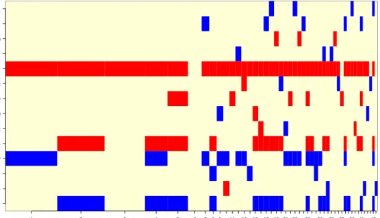
Figure Three: All Selected Models by BMA
Models selected by BMA
Model # 1 2 3 4 5 6 7 8 9 11 13 15 17 19 21 23 26 29 32 35 38 41 45 yd_sp cred_sp inf_chg inf term_sp int tbill ip_gw vol.px ern_yd div_yd jan r.lag2 r.lag1
36 Bayesian Model Averaging is a technique designed to help account for the uncertainty inherent in the model
selection process, something which traditional statistical analysis often neglects. By averaging over many different competing models, BMA incorporates model uncertainty into conclusions about parameters and prediction.
Table Four: Best Five Models from BMA
p!=0 EV SD model 1 model 2 model 3 model 4 model 5
Intercept 100 -1.4948024 4.54649 3.4166 -6.0893 -2.3283 -1.1270 -6.3758 r. l a g 1 4 . 2 - 0 . 0 0 2 2 0 6 0 . 0 1 8 6 4 . . . . . r.lag2 6.3 -0.0048645 0.02647 . . . . . jan 3.4 0 .021128 0 .22601 . . . . . d iv_y d 3 .6 -0 .116 728 1 . 13552 . . . . . ern_yd 93.9 0.8678841 0.38095 0.9267 1.0079 0.6725 1.1909 0.9656 v o l . p x 4 . 5 - 0 . 0 0 0 3 3 3 0 . 0 1 0 2 9 . . . . . ip_gr 11.3 0.0994274 0.34683 . . . . 1.0530 t b i l l 4 . 0 0 . 0 1 6 2 6 7 8 2 . 8 5 6 8 . . . . . i n t 3 . 6 0 . 0 0 2 9 0 1 0 . 0 5 7 5 6 . . . . . term_sp 42.2 1.3383220 1.75732 . 3.2756 . 2.9965 3.6263 inf 39.4 -0.6020492 0.86491 -1.5513 . . -1.2644 . i n f _ c h g 4 . 6 - 0 . 0 4 6 5 1 7 0 . 3 1 6 9 1 . . . . . c r e d _ s p 4 . 2 0 . 0 0 8 2 3 5 0 . 4 3 7 7 . . . . . yd_sp 42.3 -1.3094495 1.7177 . -3.2197 . -2.9291 -3.6052 nVar 2 3 1 4 4 BIC -728.9691 -728.8057 -728.4717 -727.3078 -727.1379 post prob 0.139 0.128 0.108 0.060 0.056 (cumulative posterior probability = 0.4908 )
Something interesting we find in BMA procedure is that the variable vol/px is left out
from most selected models, which is not consistent the results from the other criteria. This difference is probably due to the poor out-of-sample predictive power of vol/px,
despite the high correlation between vol/px and excess return. If look into the best five
models (in Table Four) with highest posterior probabilities, only the last one of them includes vol/px. Since some research has implied that posterior probabilities are more
generally supportive of stock return predictability than prior probabilities, we may conclude that vol/px has little predictive power for excess return from the results in
Table Four (on the previous page). Some might explain that the reason for different results from different criteria is the spurious high correlation between vol/px and ex.r
that should actually be attributed to the causal relation between ex.r and some other
hidden variables. Another explanation is that the correlation between vol/px and ex.r is
not linear or even not monotonic. Anyway, the out-of-sample predicting performance
of vol/px would be definitely poor, so it contributes little to the predicted excess return.
In such way, vol/px does not make a difference in our forecasting model,38 and
therefore is excluded from the basket of the candidate factors.
To sum up, after combining all the model selection criteria, the variables we finally pick up for our model are earnings yield, term spread, inflation rate and yield spread. The following section will discuss our final model concerning some important issues, such as goodness-of-fit, predictability and interpretation.
Section IV: Results Analysis
With the four chosen variables, a reduced model is fitted and the results are much better compared with the full model. An ANOVA test also suggests that the reduced model is good enough to estimate the excess return mean, while the other unfavorable
38 In fact, we try to fit both the model with
vol/px and the model without vol/px. The coefficients on the other
variables are almost the same in two models, and the coefficient on vol/px is really small and not statistically
variables together could not contribute to the model significantly. (The p-value is 0.77, far above the benchmark value 0.05 to reject the null hypothesis.) The reduced model we have is:
ex.r = 0.58 ern_yd+0.90 term_sp -0.85 inf -0.89 yd_sp+0.92 (0.23) (0.87) (0.63) (0.85)
× × × ×
Most of the coefficients are significant at the level of 0.10. Although this model might not be conclusive, it truly provides us a general idea of the stock return forecast model and gives out an intuitive interpretation of the predictive power of the selected variables. The signs of the estimated coefficients also provide us some important information about the variables, which might help us to tell the direction of market excess return changes.
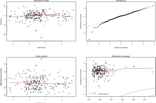
To check goodness-of-fit of this model, several tests are carried out and the results (in Figure Three on next page) are showing that the model is well fitted. The residual plots, especially the standardized residual plot39, have no particular pattern, indicating the character of white noise. The normal Q-Q plot40 is also in support of the normality of residuals, but the shape of two ends suggests the distribution for residuals are actually long-tailed. The leverage plot finds the two leverage points – No.91 and No.221, which explain the long-tailed shape. If we investigate the two observations, we will find they are two extreme cases: No.91 flags the stock market crash in the Oct of 198741, and No.221 represents the financial crisis aroused by hedge funds starting from Sep of 1998. Even though the extremely influential cases can be identified in our data, nothing needs to be done with them as the fit model will not change much.
39 Standardized residual plot is the plot on the lower left quarter, and the regular residual plot is on the upper left. 40 Q-Q normal plot is on the upper right quarter.
41 The stock market crash of 1987, also known as black Monday, was the largest one day stock market crash in
Figure Three: Residuals Studies -1 0 1 2 -2 0 -1 0 0 1 0 Fitted values R es idual s Residuals vs Fitted 91 221 270 -3 -2 -1 0 1 2 3 -4 -2 0 2 Theoretical Quantiles S tanda rdi z ed r es idual s Normal Q-Q 91 221 270 -1 0 1 2 0. 0 0. 5 1. 0 1. 5 2. 0 Fitted values S tandar di z ed r es idual s Scale-Location 91 221 270 0.00 0.02 0.04 0.06 0.08 0.10 -6 -4 -2 0 2 Leverage S tan dar di z ed r es id ual s Cook's distance Residuals vs Leverage 91 221 251 1 0.5
Now we make sure that the model is good for fitness, but whether it is good for predictability, especially the out-of-sample predictability, is another important concern about the model. As the in-sample predictability is self-checked by the model selection criteria42, we only need to investigate the out-of-sample predicting power. Here, the10-Fold Cross Validation needs to introduced to check the out-of-sample predicting ability. This method randomly divides the data into ten groups, and then fit the model using nine tenths and compute prediction error on the remaining one tenth. The process will be repeated ten times to get each one tenth calculated for the predication error. Averaging the ten prediction errors, a statistic - mean square error (MSE43) is obtained, which can be used for comparing different model at the same time. From the table on the next page (Table Five), we could see several good results
42 The model selection criteria applied in the last section just select the model with best in-sample predictability. 43 MSE of an estimator is one of many ways to quantify the amount by which an estimator differs from the true
value being estimated. As a loss function, MSE is called squared error loss. MSE measures the average of the square of the "error." The error is the amount by which the estimator differs from the quantity to be estimated.
from cross validation method, with relatively small values for MSE. The best model is our reduced model, including the variables we selected in the last section – ern_yd,
term_sp, inf and yd_sp.
Table Five: 10-Fold Cross Validation
r.lag1 r.lag2 jan div_yd ern_yd vol/px ip_gr tbill int term_sp Inf inf_chg cred_sp yd_sp mse
0 0 0 0 1 0 0 0 0 1 1 0 0 1 14.01 0 0 0 0 1 0 1 0 0 1 0 0 0 1 14.24 0 0 0 0 1 0 1 0 0 1 1 0 0 1 14.24 0 0 0 1 1 0 1 1 0 1 1 0 0 1 14.11 0 1 1 0 1 0 1 0 1 1 1 0 0 1 14.10 0 1 1 0 1 0 1 0 1 1 1 1 0 1 14.18 1 0 0 1 1 0 1 0 0 1 0 0 0 1 14.21
However, we find that even this best model we have is not good enough for out-of-sample prediction. The square root of MSE value is almost as large as the standard deviation of the excess return. That is to say, the prediction made from this model is not much better than just picking the mean value of excess return. Such conclusion is disappointing, and we have to find some way to improve the predictive performance, if there is a way to do so.
One way we tried is to include the interaction in hope for discovering nonlinear correlation between the variables, but it does not work out very well.44 Then another thought occurs to us that some other influential factors for the stock market could be added into our model, since some of the variation in excess return might not explained
by our model due to the omission of some crucial factors. The volatility expectation, which has rarely been used in research up to now, is our choice, because it reflects how speculative the stock market is and would affect the rational behavior of investors as well. In the following section will discuss our new model with the volatility expectation variables and focus on whether improvement in out-of-sample predicting ability is found.
Section V: Model Improvement
As we already mentioned in Section II, there is an index measuring the volatility expectation of the stock market – Volatility Index which can be added in our model directly. However, the only problem here is that some of the observations are lost here, since the volatility index data is only available from year 1990. If this variable is used, we have to truncate all the data to make all the variables go with each other. Another way to get access to the expected volatility is to estimate it through historical data. The theory of rational investor behavior makes us believe that people will adjust their expectation for volatility according to the actual market volatility. It is not hard to understand that when the stock returns are relatively volatile for the whole market, more speculation and trading in the financial markets might happen, leading to a higher expectation for volatility. Concerning about the time horizon, one month is long enough to make people react to the market, so the monthly volatility data could be a good estimator for the volatility expectation for the next month.
Besides the expected volatility variable, the change in expected volatility that could be interpreted as the shock to volatility expectation might also affect the excess return in the next period. Intuitively, the unexpected volatility in the stock market could
greatly influence the behavior of investors, which part can not be explained by rational decision behavior. What happened in the financial crash could be a perfect example for this: some unexpected downside trend in the volatile market aroused severe drops in the stock market, ending with an even higher volatility of the market. Such unexpected volatility variable acts the role of amplifier in the excess return predicting model, and it probably not only has the main effect on excess return but also interacts with the other crucial variables already in the model. Thus, the interaction terms of volatility variable and other variables will also be considered in the candidate models.
To test whether the expected or unexpected volatility indeed has the predicting power for excess return as we analyzed, the volatility-related variables should be added into the reduced model with interaction terms, and several sets of new models needs to be constructed and compared with each other. Since the data horizon is not the same as that used in the sections before45, we also need to refit the reduced model to set up a new base model to compare with. For the selection criterion, we only use the 10-Fold Cross Validation method in this section, as it is the only criterion takes the out-of-sample predictability into model selection procedure. In addition, the statistic MSE obtained from cross validation can be used to compare all the models, as long as the models are fitted, using observations46 over the same time period. The meaningful interpretation for the statistic MSE can also help us to understand the model fitness and the predicting ability of the model.
Studying the results from different models (in Table Six on the next page), in which the base model and the four best selection results for each model are listed, we could
45 There is loss of observations due to the unavailability of the volatility index value. 46 No missing value should be in the data set.
compare all the improved models at the same time. Notice that all the interaction terms are considered in the candidate model set. The best model of all is the reduced model with the variable of unexpected volatility added in but no interaction terms included.
Table Six: Reduced Model + Volatility Factor Reduced Model + vix47:
ern term inf yield vix ern* term* inf* yield*48
MSE
Reduced Model + unvix49:
ern term inf yield unvix ern* term* inf* yield* MSE
1 1 1 1 0 0 0 0 0 15.018 1 1 1 1 1 0 0 0 0 14.810 1 1 1 1 1 0 0 8 0 15.053 1 1 1 1 1 0 0 8 9 14.959 1 1 1 1 1 0 7 0 0 14.999 1 1 1 1 0 0 0 0 0 15.018 1 1 1 1 1 0 0 0 0 14.744 1 1 1 1 1 6 0 0 9 14.601 1 1 1 1 1 6 0 8 0 14.656 1 1 1 1 1 0 7 8 0 14.759
Reduced Model + vol50:
ern term inf yield vol ern* term* inf* yield* MSE
Reduced Model + unvol51:
ern term inf yield unvol ern* term* inf* yield* MSE
1 1 1 1 0 0 0 0 0 15.018 1 1 1 1 1 0 0 0 0 14.805 1 1 1 1 1 0 0 0 9 15.116 1 1 1 1 1 0 0 8 0 15.145 1 1 1 1 1 0 7 0 0 15.093 1 1 1 1 0 0 0 0 0 15.018 1 1 1 1 1 0 0 0 0 13.863 1 1 1 1 1 0 0 8 0 14.190 1 1 1 1 1 6 0 0 0 14.165 1 1 1 1 1 6 7 0 9 14.426
The results consistently support that the volatility variables matters for predicting
47
vix refers to the volatility index which measures the volatility expectation of the market.
48 The star on shoulder of the variable indicates that the variable is timed with the newly added volatility
variable.
49
unvix refers to the change in volatility index which measures the shock to the volatility expectation (a.k.a.
unexpected volatility).
50
vol refers to the alternative volatility expectation variable estimated by the historical market volatility data. 51 unvol refers to the change in volatility expectation variable which is an alternative to unexpected volatility.
excess return, because the best model selected in each set includes the volatility variable. Apparently, the unexpected volatility does a better job, and when both of them included in the model, the unexpected volatility is also preferred by selection criteria. In such a way, we provide some evidence for our argument that the unexpected volatility can impact the stock market greatly so as to influence the market excess return. Besides, the cross validation also tells that the models with unexpected volatility variable have better predictability (both the in-sample and the out-of-sample predictability, which are reflected in the goodness-of-fit measurement and MSE statistic respectively).
It is obvious that the model is better fitted and has better predictive performance, since the MSE is dropped nearly 2 points, which is considered to be significant improvement. However, this better model might yet not be applicable in practice: the root of mean square error is about 3/4 of the standard deviation of the excess return, which means the prediction does not work quite well either, especially when the model is used for prediction52. There is no standard to measure whether the mean square error is acceptable, but reducing MSE would always be our purpose.
Section VI: Conclusion
The theory that stock excess return is predictable uncovered in the empirical financial study has a huge effect on financial research in the past three decades. The predictive power of some financial and economic factors has found supportive evidence in the academic research results. The theoretical progress is also applied to the empirical work, and therefore many models has been built to predict such excess return, and
these models are widely used by all kinds of investors. In this article, we investigate the claims of the predictability of stock excess return by fitting the equilibrium model with all the potential variables.
Several model selection criteria are employed to decide the model, the positive result is that the models selected by different criteria are quite consistent with each other. The variables with prominent predicting power stand out clearly, and the model including them is well fitted. However, there is also bad news with the fitted model that its out-of-sample predictability performs badly, as what has been argued in some previous literature. Even the best model selected by cross validation53 which takes into consideration the out-of-sample predictability issue does not give out a better forecasting model for market excess return than the constant model (mean of the historical market excess return).
In order to improve the model, especially to have a better out-of-sample predictability, some volatility-related is considered to be included in our model. In hope to find some expectation effect or shock effect of volatility on the stock market, we refit the model by adding in the new variables with the interaction terms to the obtained model. Comparing all the candidate models at the same time, the model with unexpected volatility variable is the one with the best out-of-sample predictability. The new model obviously has better performance for prediction, but yet it is far from satisfaction as the mean square error for prediction is still quite large.
Although not good enough, the new model clearly tells us that the unexpected volatility which has rarely been used in previous research has predictive power on
stock market excess return. This could leads to some further research about this factor or even some other influential variables on investors’ rational behavior. From this aspect, the stock market might be also affected by some factors out of the economic or financial scope. However, the correlation can be really complicated and therefore the nonlinear model might apply. Anyway, we believe that the volatility expectation, actually the change in volatility expectation does make a difference in predicting the market stock excess returns.
Before reaching the final conclusion, the limitations on our models should be discussed. First of all, we presume the requirements for linear regression are met, such as normality54, linearity55, parameter stability56. Secondly, the data snooping may persistently exist, even if we try the best to limit the overfitting possibility by employing Akaike’s information criterion and Bayesian framework to select the model. The last but not the least is that our idea of volatility expectation variable is raw, and the variable might not be appropriately estimated with the historical data, since the expectation may not always be adjusted according to what just happened. A lot of outside information which cannot be measured directly might have impact on the expected volatility, and we have to ignore that. In addition to what we have discussed, the correlation between expected/unexpected volatility and market excess return is probably nonlinear, as the rational behavior impact can be complicated.
However, we believe that the results from our simple model will not be dominated by these bias or other limitations. For the prerequisites for linear regression, an afterwards test is taken out: the variable distributions are following the similar shape,
54 Normality refers to the normal distribution of the observation for variables.
55 Linearity refers to the linear relationship between the explanatory variables and the response variable. 56 Parameter stability refers to the fact that the model parameters do not change over time.
and the large sample size makes the normal distribution requirement not necessary; from the pair scatter plot57 of the chosen variables, the linear relationship between them is clear shown; the parameter stability is not tested in the article, but if the variables have the consistent effect, then they should not change too much. For the data snooping problem, we have tried best to model against it with model selection criteria, and as long as the theoretical support is found, there is no need to worry about this problem. For the volatility variables, we already show that the main effect exists, and the non-linear part can be left for extensive research.
With the model we obtain, the interpretation is quite straight forward. To summarize, some financial and economic factors are found to have predicting power on market excess return in this article, and such predictive power can also be found for market unexpected volatility variable. With the unexpected volatility, our model can be improved to have better in sample and out-of-sample predictability, but yet it needs further extension. In any case, our model provides some interpretation of the investors’ rational behavior effect on the stock market through the unexpected volatility variable which has not been discussed in the previous literature and may be investigated more in the future research.
References
Abhyankar, A., L.S. Copeland, and W.Wong, 1997 “Uncovering Nonlinear Structure in Real-Time Stock Market Indices”, Journal of Business and Economic Statistics, 15 (1): 1–14.
Akaike, H., 1974, "A New Look at the Statistical Model Identification," IEEE Transactions on Automatic Control,
AC-19, 716723.
Ang A., and G. Bekaert, 2006, “Stock Return Predictability: Is It There?” working paper.
Bossaerts, P., and P. Hillion, 1999, "Implementing Statistical Criteria to Select Return Forecasting Models: What Do We Leam?” Review ofFinancia1 Studies, 12, 405428.
Campbell, J. Y., and M. Yogo, 2006, "Efficient tests of stock return predictability”, Journal of Financial Economics, 81 (2006): 27-60.
Chen, N., R. Roll, and S. Ross, 1986, "Economic Forces and the Stock Market," Journal of Business, 59,
383403.
Chiarella, C., W. Semmler, S.Mittnik and P. Zhu, 2002, “Stock Market, Interest Rate and Output: A Model and Estimation for US Time Series Data”, Studies in Nonlinear Dynamics &Econometrics, 2002, vol 6.
Fama, E. F., 1991, "Efficient Capital Markets: 11," Journal of Finance, 46, 1575-1618.
Ferson, W., 1990, "Are the Latent Variables in Time-Varying Expected Returns Compensation for Consumption
Risk?'Journal of Finance, 45, 397430.
Ferson, W., and C. Harvey, 1991, "The Variation of Economic Risk Premiums," Journal of Political Economy,
99, 385415.
Ferson, W., and C. Harvey, 1993, "The Risk and Predictability of International Equity Returns," Review of Financial Studies, 6, 527-566.
Ferson, W., and C. Harvey, 1999, "Conditioning Variables and the Cross-Section of Stock Returns:' Journal of Finance, 54, 1325-1360.
Wiley, New York.
Harvey, C. R., 1989, "Time-Varying Conditional Covariances in Tests of Asset Pricing Models," Journal of Financial Economics, 24, 289-317.
Hawawini, G., and D. B. Keim, 1995, "On the Predictability of Common Stock Returns: Worldwide Evidence,"
Handbooks in OR and MS, vol. 9, Elsevier Science, North-Holland, 497-545. The Review of Financial Studies,v
15 n 4 2002
Laud, P. W., and J. G. Ibrahim, 1996, "Predictive Specification of Prior Model Probabilities in Variable Selection," Biometrika, 83, 267-274.
Lettau, M., and S.V. Nieuwerburgh, 2007, “Reconciling the Return Predictability Evidence”, forthcoming: Review of Financial Studies.
Lewellen, J., 2004, “Predicting returns with financial ratios”, Journal of Financial Economics, 74 (2004): 209-235.
Lo, A,, and A. C. MacKinlay, 1990, "Data-Snooping Biases in Tests of Financial Asset Pricing Models,"
Review of Financial Studies, 3, 431467.
Lo, A,, and A. C. MacKinlay, 1997, "Maximizing Predictability in the Stock and Bond Markets," Macroeconomic Dynamics, 1, 102-134.
MacKinlay, A. C., and L. Pastor, 2000, “Asset Pricing Models: Implications for Expected Returns and Portfolio Selection,” Review of Financial Studies, 13, 883-916.
Madigan, D., and A. E. Raftery, 1994, "Model Selection and Accounting for Model Uncertainty in Graphical Models Using Occam's Window," Journal of the American Statistical Association, 89, 1535-1546.
Martijn Cremers, K. J., 2002, “Stock Return Predictability: A Bayesian Model Selection Perspective”,The Review of Financial Studies, Vol. 15, No. 4. (Autumn, 2002), pp. 1223-1249.
McMillan, and G. David 2001,“Nonlinear predictability of stock market returns: Evidence from nonparametric and threshold models”, International Review of Economics & Finance, 10 (2001) 353–368
Merton, R., 1987, "On the Current State of the Stock Market Rationality Hypothesis," in R. Dornbusch, S. Fisher, and J. Bossons (eds.), Macroeconomics and Finance: Essays in Honor of Franco Modigliani, MIT
Mitchell, T. J., and J. J. Beauchamp, 1988, "Bayesian Variable Selection in Linear Regression," Journal of the American Statistical Association, 83, 1023-1036.
Pastor, L., 2000, "Portfolio Selection and Asset Pricing Models," Journal of Finance, 55, 179-224.
Pastor, L., and R. F. Stambaugh, 2000, "Comparing Asset Pricing Models: An Investment Perspective," Journal of Financial Economics, 56, 353-381.
Pesaran, M. H., and A. Timmermann, 1995, "Predictability of Stock Returns: Robustness and Economic Significance," Journal of Finance, 50, 120 1-1 228.
Pontiff, J., and L. D. Schall, 1998, "Book-to-Market Ratios as Predictors of Market Returns," Journal of Financial Economics, 49, 141-160.
Qi, M., and G.S. Maddala, 1999, “Economic factors and the stock market”, Journal of Forecasting, J. Forecast. 18,
151-166(1990).
Raftery, A. E., D. Madigan, and J. A. Hoeting, 1997, "Bayesian Model Averaging for Linear Regression Models," Journal of the American Statistical Association, 92, 179-191.
Richardson, M., 1993, "Temporary Components of Stock Returns: A Skeptic's View," Journal of Business and Economics Statistics, April, 199-207.
Schwarz, G., 1978, "Estimating the Dimension of a Model," Annals of Statistics, 6, 41W64
Stambaugh, R. F., 1999, "Predictive Regressions:' Journal of Financial Economics, 54, 375421.
Taylor, S.J. 1994, “Modeling Financial Time Series” Chichester: J. Wiley & Sons .
Thaler, R.H., 1987, “The January Effect”, The Journal of Economic Perspectives, Vol. 1, No. 1. (Summer, 1987),
pp. 197-201.
Whitelaw, R., 1994, "Time Variations and Covariations in the Expectation and Volatility of Stock Market Returns," Journal of Finance, 49, 515-541.
Zellner, A,, 1986, "On Assessing Prior Distributions and Bayesian Regression Analysis With g-Prior Distributions,"