Support Vector Machines in HTS Data Mining:
Type I MetAPs Inhibition Study
JIANWEN FANG,1,2
YINGHUA DONG,1
GERALD H. LUSHINGTON,1,3
QI-ZHUANG YE,4
and GUNDA I. GEORG4
This article reports a successful application of support vector machines (SVMs) in mining high-throughput screening (HTS) data of a type I methionine aminopeptidases (MetAPs) inhibition study. A library with 43,736 small organic molecules was used in the study, and 1355 compounds in the library with 40% or higher inhibition activity were considered as active. The data set was randomly split into a training set and a test set (3:1 ratio). The authors were able to rank compounds in the test set using their decision values predicted by SVM models that were built on the training set. They defined a novel score PT50, the
percentage of the test set needed to be screened to recover 50% of the actives, to measure the performance of the models. With carefully selected parameters, SVM models increased the hit rates significantly, and 50% of the active compounds could be recovered by screening just 7% of the test set. The authors found that the size of the training set played a significant role in the performance of the models. A training set with 10,000 member compounds is likely the minimum size required to build a model with reasonable predictive power. (Journal of Biomolecular Screening2006:138-144)
Key words: support vector machines, high-throughput screening, MetAP, machine learning
INTRODUCTION
I
N THE PAST DECADE, the application of combinatorial chemistry and parallel synthesis in drug discovery has generated enor-mous collections of small organic molecules.1,2Automated screen-ing operations have significantly speeded up the primary testscreen-ing stage; still, it has remained a formidable challenge to screen all combinations of the tremendous number of available compounds and the fast-growing number of targets, thanks to the successfully sequenced human genome. Recently, the concept of “smart screening,” instead of brute-force screening, has attracted much at-tention.3
There is a growing movement toward using in silico tech-niques as a means to complement wet lab screening. These compu-tational activities can be grouped into the following categories:
(a) Prescreen filtering: use empirical or theoretical rules (e.g., the
fa-mous Lipinski “rule of 5”4) to filter drug-like candidates.
(b) Docking simulations: if the 3D structure of the biological target is available, a docking study can be performed to identify molecules that have potential high binding affinity to the target. This
proce-dure can be used as prescreening filtering step or in parallel with experimental screening efforts.
(c) Data-mining screening results: predictive models using statistical or machine-learning approaches based on screening results of small libraries are used to select likely active compounds from large libraries. This type of activity is similar to conventional quan-titative structure-activity relationship (QSAR) studies. However, in most cases, simply scaling up QSAR from a few dozen similar compounds to thousands of compounds would fail. Two major rea-sons contribute to the likely failure: (1) a library used for a high-throughput screening (HTS) study usually has thousands of com-pounds (or more) with diverse physical properties and structural features that cover substantial chemical space. Because the fea-tures that dictate activity in some subsets of molecules may be completely absent in other (sometimes comparably active) subsets, the current correlation schemes underlying QSAR technologies work better only for compounds with similar structures. (2) HTS screening data are noisy and tend to be polluted, to a certain extent, with false positives and false negatives. In contrast, the smaller scale assays used for QSAR studies are likely to be more accurate because the activities of the compounds are often determined by
in-dividual experiments based on more data (e.g., by IC50
determinations). In this sense, only methodologies that can tolerate noisy data can be used in HTS data mining.
Machine-learning techniques have been applied in HTS data mining in recent years.5For example, recursive partitioning (RP) and various types of artificial neural networks (ANN) have been used for analyzing HTS data sets.3,6Recently in the machine-learning community, the support vector machine (SVM) has gained much attention due to its superior performance and proven 1
Bioinformatics Core Facility,2
Information and Telecommunication Technology Center,3
Molecular Graphics and Modeling Laboratory, and4
High Throughput Screening Laboratory, University of Kansas, Lawrence.
Received Jun 15, 2005, and in revised form Oct 27, 2005. Accepted for publica-tion Nov 2, 2005.
Journal of Biomolecular Screening 11(2); 2006 DOI: 10.1177/1087057105284334
robustness for noisy high-dimensional data.7SVM has been used to build QSAR models, often with better predicting power than other machine-learning methods such as neural networks, radial basis functions, and decision trees.8-10Nevertheless, the applica-tions of SVM to large-scale data analysis have generated some-what contradicting results. For example, Byvatov and coworkers11 applied SVM and ANN to a drug/nondrug classification problem. They found that both methods gave satisfactory results, whereas SVM gave a slightly higher prediction accuracy than the ANN sys-tem. Very recently, Muller et al.12dramatically improved the SVM models on the same data set via carefully selecting model parame-ters. On the other hand, Wilton and Willett13applied SVM in the analysis of the National Cancer Institute’s AIDS data set and found SVM “markedly inferior” as compared to other ranking methods tested in their study. However, the poor performance was likely a consequence of a very small training data set. Another reason might be that the authors did not optimize the parameters of SVM models.
In this article, we describe a successful application of SVM in the type I methionine aminopeptidases (MetAPs) inhibition HTS screening data analysis. MetAPs are metalloproteinases responsi-ble for removal of the N-terminal methionine residue from newly synthesized protein molecules and are essential for survival of all cell types.14
They have been suggested as promising targets for an-tibacterial, antifungal, and anticancer agents.
METHODS Compound library selection
The library of 43,736 small organic molecules used in the study was a carefully selected collection targeted at successful identifica-tion of lead compounds. The compounds were purchased from ChemBridge (San Diego, CA), and the compounds were screened from its Express-pick collection of 230,000 compounds. In addi-tion to consideraaddi-tion of the Lipinski rules,4
the selection process drew upon specific chemical knowledge. Reactive, unstable, and potentially toxic compounds, such as esters, amides, acid chlo-rides, Michael acceptors, and poly-aromatics, were eliminated, and all compounds were solids with molecular weights between 150 and 480 dmu and cLogP values below 5.
Assay for methionine aminopeptidase inhibitors
The assay for methionine aminopeptidase inhibitors was re-ported previously.14
In brief, recombinantEscherichia coliMetAP was purified as an apo-enzyme and then activated with a divalent metal [Co(II)]. A continuous assay with fluorogenic Met-AMC as the substrate was used for the screening, and hydrolysis was moni-tored by recording fluorescence (excitation at 360 nm and emis-sion at 460 nm) every 3 min in a period of 30 min. All compounds were screened at a concentration of 6.67µg/mL. The assay pro-duced 1355 active hits (40% or higher inhibition as measured by fluorescence).
Descriptors generation and selection
To predict molecular activities, it is important to use suitable descriptors relevant to the biological problem. In this study, we used a collection of molecular descriptors calculated using Qua-SAR-Descriptor in the Molecular Operating Environment (MOE, Chemical Computing Group, Inc., Montreal, Canada). The MOE descriptor set includes 219 features that can be partitioned into 3 classes:
2D descriptors:this class of descriptors is calculated from the atoms and connection information of the molecule. No 3D conformation information is considered. All descriptors in the class are numeri-cal properties and include physinumeri-cal properties, subdivided surface areas, atom counts and bond counts, Kier & Hall connectivity and Kappa shape indices, adjacency and distance matrix descriptors, pharmacophore feature descriptors, and partial charge descriptors.
Internal 3D descriptors:this class uses 3D coordinate information and includes potential energy descriptors, surface area, volume and shape descriptors, and conformation-dependent charge. These descriptors are invariant to rotations and translations of the conformation. The internal 3D descriptors require that the mole-cules have reasonable conformations. For this purpose, the MOE 3D-Converter was used to minimize the conformations of the compounds.
External 3D descriptors:this class requires an absolute frame of refer-ence (e.g., molecules docked into the same receptor). Because the orientation of many of the active ligands binding to the receptor is unknown, this class of descriptors was not considered in the study.
Because it is difficult to predict in advance which descriptors are most relevant to the problem at hand, a feature selection (FS) procedure may be desirable.15However, SVM is well known to tol-erate irrelevant features.16-18In some cases, the best average perfor-mance was achieved when all the features were given to SVM.19In this study, only exactly duplicated features for all compounds in the library were eliminated, and the procedure generated a set of 203 features.
Support vector machines
The support vector machine algorithm was developed by Vapnik.7
SVMs are the first mathematical models that do not as-sume any specific probability distributions and that learn from ex-perimental data. SVMs adopt the structure risk minimization (SRM) principle developed by Vapnik that has been demonstrated to be superior to the traditional empirical risk minimization (ERM) principle that has been used by conventional neural networks. SRM minimizes an upper bound of the prediction error based on the Vapnik-Chernovenkis (VC) dimension, as opposed to ERM, which minimizes the training error. A number of review articles and tutorials on SVMs have been made available,20
and thus only the basic theory of SVMs for binary classification is briefly reviewed in the following section.
An SVM model identifies the maximum margin of a hyperplane separating 2 classes. Mathematically, given a training set of (xi,yi),i= 1, . . .,n, wherexiis an instance andyiis its label, the
SVM model can be trained by solving the following optimization problem: Minimize || ||ω 2 ξ 1 + =
∑
C i N i Subject toyi(ω•φ(xi) +b)≥1 –ξi, ξi≥0whereCis a constant that determines the trade-off between the smoothness of the model and the toleration of deviations,ξiare nonnegative variables that are used to measure the misclassification errors,ωis normal to the hyperplane, ||ω||2is a term that characterizes the model complexity, andbis the SVM bias term.K(xi,xj) =φ(xi) •φ(xj) is known as the kernel function, which allows nonlinear mapping by projecting descriptors onto the feature space. All kernel functionsK(xi,xj) must satisfy Mercer’s condition that corresponds to the inner product of some feature space.21A number of kernel functions, including linear, polyno-mial, radial basis function (RBF), and sigmoid, have been used in SVM models. The RBF kernel (e−γ||x−y||2) is by far the most popu-lar choice in SVMs because its response is localized and finite across the whole range of real numbers. As well, the RBF has only one hyperparameterγto be determined by training.
In this article, we used SVM as implemented in LIBSVM.22
RBF kernels were used for the reasons described in the previous paragraph. We used a 2-stage grid selection to determine the smoothness trade-off parameterCand the RBF scale parameterγ. IfCis too large, the model risks overfitting the training data. IfCis too small, then the model may underfit the training data. The value ofγcontrols the amplitude of the kernel function. An overly large value ofγmay lead to the overfitting problem, whereas a small value may produce boundaries for classifying training examples that are too smooth to exhibit sufficient accuracy. Thus, usually “better” regions exist for both ofCandγ.
We also modified and recompiled the LIBSVM source code to access the decision values.22
The decision values are the relative perpendicular distances of the predictions from the separating hyperplane, where higher scores are more favorable. The standard LIBSVM uses the signs of decision values to perform binary clas-sification. Here we demonstrated that SVM can also be used in ranking problems via direct use of the decision values.
Performance evaluation
The goodness of predictions is frequently measured by sensi-tivity (the percentage of active compounds that were correctly classified), specificity (the percentage of inactive compounds that were correctly classified), and prediction accuracy rate. However, considering any one of these measures alone could be very mis-leading for unbalanced data generated from a typical HTS experi-ment. For instance, given an HTS data set with 3% active com-pounds, simply classifying all compounds as inactive will result in a 97% prediction accuracy rate on an inactive data set.
In this study, we defined a novel score PT50, the percentage of
the test set needed to be screened to recover 50% of the actives, to
measure the performance of the models. We calculated the deci-sion values and used them to rank the compounds in the test data set. We also used decision values to generate a receiver operating characteristic (ROC) curve that is a plot of the true-positive rate (sensitivity) against the false-positive rate (1 – specificity). The area under an ROC curve represents the trade-off between sensitiv-ity and specificsensitiv-ity. In general, an area of 1 represents a perfect pre-diction model, and an area over 0.9 is considered excellent. An area between 0.8 and 0.9 is considered good, whereas the range of 0.7 to 0.8 is fair.
In addition, we calculated Matthews’s correlation coefficient (CC):23
CC=(NP OU− ) (N+O N)( +U P)( +O P)( +U).
P,N,O, andUrefer to true-positive, true-negative, false-positive, and false-negative predictions, respectively. The values ofCCcan range from 1 for perfect prediction to –1 for no prediction power.
RESULTS
The set of 43,736 compounds was randomly split into 2 sub-groups in a 3:1 ratio. The larger subgroup was used as a training set and the smaller as a test set. We then randomly selected 4000, 10,000, 20,000, and 30,000 compounds from the training group to probe the influence of the size of the training data on the parameter selection and performance of the models. The test data set was not used in the training procedure.
Grid-selectingCand
Because the smoothness trade-off parameterCand the RBF scale parameterγwere not known beforehand, we conducted ex-tensive grid searches to optimizeCandγin order to build powerful models to predict unseen data. Five-fold cross validation was used in our experiments to determine these parameters. The training data set was randomly split into 5 equal portions. One portion was reserved for the test data, and the rest was used for the training data. This was repeated for each possible validation fold, and thus every compound was used in prediction once. The results were then av-eraged. It should be stressed that only the data from the original training data set were used in subpartitioning into cross-validation training and test sets. We conducted a 2-stage grid-selecting pa-rameter process. The first stage was a crude search in which we screened all combinations of the followingCandγ:C= 2–5
, 2–3 , 2–1 , 2, 23 , 25 , 27 , 29 , 211 , 213 , 215 andγ= 2–15 , 2–13 , 2–11 , 2–9 , 2–7 , 2–5 , 2–3 , 2–1 , 2, 23
on 4K and 20K training data sets. The results from cross-validation tests confirmed that both data sets resulted in similar “better” regions ofCandγ, as the authors of LIBSVM suggested,22
although the performance of the larger data set was generally the best (Fig. 1).
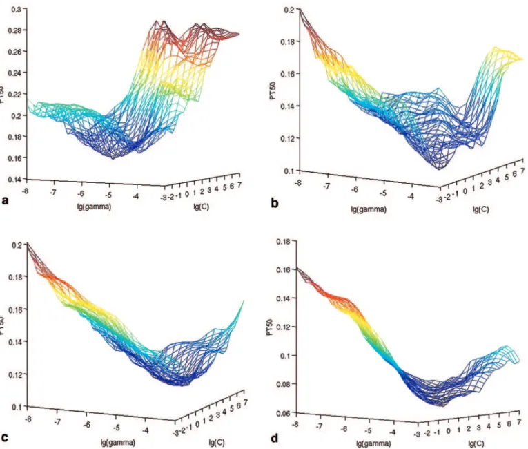
The second stage was a better-region-only grid search on all 4 data sets to determine optimal parameters for each of them (Fig. 2). The selected parameters (Table 1) were then used to build models
based on each training data set, and the models were tested on the same test data set.
The performance of models
Table 1summarizes the predictive performance of SVM mod-els on the test data set. All measures (PT50, ROC area, andCC
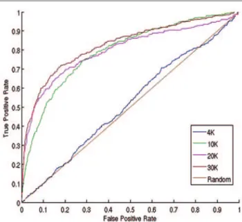
value) pointed out that the size of the training data set played a sig-nificant role in the performance of the models. The model built on the smallest training data set had almost no predictive power (Fig. 3). The performance improved quickly as the size of the training set grew. We found that a training set with 10,000 members likely covered substantial chemical space and thus yielded appreciable predictive power. The best model, built on the 30K training data set, would allow us to recover 50% of the actives by screening 7.1% of the test set, which indicated about a 7-fold hit rate im-provement over random selection. We also calculated the concen-tration of true-positive hits in the top 1% and 5% of rankings ( Ta-ble 2). The model that resulted from the 30K training set showed that 48.6% of top 1% predictions were correctly classified, which was a 16-fold increase over random selection.
DISCUSSION
SVM is a machine-learning approach that allows one to learn from experimental data within a given set and then build a com-puter model to make predictions on new data sets. Our study dem-onstrated that a careful model selection procedure can improve the results dramatically. We also demonstrated that SVM was also ap-plicable to ranking putative activities of compounds via decision values.
Model selection
SVM model selection consists of 2 steps: choosing a kernel function and defining its parameters. RBF is by far the most widely used kernel function for mapping nonlinear samples into a higher dimensional space because of its mathematical simplicity and su-perior performance over other functions. The systematic search and selection of the penalty parameterCand kernel parameterγ should be considered as an unavoidable step of model selection. Table 3compares the PT50of models using default parameters to
those with optimized parameters. The trial using a model with de-fault parameters needed 117% more compounds to recover 50% of active compounds. Although a “grid search” is computationally expensive, it is the most reliable approach for optimizing parame-ters. Conducting a coarse grid search on a smaller, randomly se-lected training subset to determine a “better” region first is a practi-cal cost-saving approach. In our study, on average, it took 21 and 5 sec, on a 64-bit quad system (2.4-GHz AMD Opeteron, 16 GB
FIG. 1. Crude grid searches ofCandγ. Left graph is the average PT50of cross-validation tests for the 4K training data set, and right one is for the 20K set. Both have similar “better” regions.
Table 1. Optimized Parameters on Different Training Sets and the Prediction Performance of the Models
Based on the Parameters and Data Sets
Lg(C) lg(γ) PT50 ROC Area CC
4K 1 –6 0.478 0.516 0
10K –1.5 –3.5 0.120 0.793 0.197
20K 4 –4.5 0.0746 0.797 0.287
30K –0.5 –3 0.0710 0.827 0.287
RAM, RedHat AS LINUX), to run a cross-validation training and test on the 4K data set, which was significantly shorter than 762 and 151 sec on 20K data set, respectively.
Model complexity and training error
Most modern machine-learning methods consider the trade-off of the model complexity and training errors. Simple models do not have good representational power and may give high training er-rors. However, they may tolerate noisy data so that they do not de-pend heavily on the particular training data set used. On the other hand, complex models may deliver reduced training errors, but they may model not only the data but also the inherent noise. Thus,
complex models may not have good prediction power on unseen data if the training data are contaminated with noise. In other words, complex models are more likely to overfit data. Techniques such as cross-validation have been used to address the overfitting
FIG. 2. Fine grid searches of parametersCandγ. Average PT50of cross-validation on the (a) 4K training set, (b) 10K training set, (c) 20K training set,
and (d) 30K training set. All of them have a different global minimum.
Table 2. Concentration of True Positives (TP) in the Top 1% and 5% of the Ranking
4K 10K 20K 30K
%TP in top 1% rank 2.7 28.8 42.3 48.6
problem. However, one should keep in mind that cross-validation is similar to real prediction but is not identical. This fact was appar-ent in this study, where the cross-validation on the 4K training set showed some prediction power, but the power vanished in predicting activity within the test set.
The size of training data set matters
As discussed in the Introduction, one of the biggest differences of HTS data analysis as compared to traditional QSAR is that HTS analysis deals with a compound library that is designed to be not only structurally very diverse but also sufficiently replicated in terms of chemical features, which is required but unnecessarily sufficient to ensure that the important molecular features are iden-tified by a machine-learning model. From our study (Table 1and Fig. 3), it seems that a random library with about 10,000 member compounds is required to build a model with reasonable predictive power. Considering the hundreds of available molecular features, we do not believe models built with only a few hundred compounds would perform well.
CONCLUSION
In this article, we have reported a successful application of the SVM method in HTS data analysis. Our experiments suggest that the application of this promising technology provides an effective way of prioritizing compounds for biological testing after an initial screen of sufficient size has been run. We also demonstrated that the newly defined score PT50 is applicable in evaluating the
performance of models.
Although extensive analyses have been carried out in the study, there is still plenty of room for further improvements. For example, a feature selection procedure may be desirable to improve the effi-ciency of the models. Also, there are many additional descriptors that can be calculated using commercial or academic software pro-grams. Without knowing what features are relevant, it is beneficial to screen features in addition to those in MOE. By ranking fea-tures, we may acquire better insight as to which features are impor-tant for the biological activities under study. Such additional stud-ies are currently under way and will be reported elsewhere.
ACKNOWLEDGMENTS
This work was supported by the K-INBRE Bioinformatics Core, NIH grant number P20 RR016475, P20 RR-17708, RR015563, RR016475, and AI065898. We thank Dr. Chih-Jen Lin from National Taiwan University for his useful suggestions. We also thank the editor and the 2 anonymous reviewers for their thoughtful suggestions.
REFERENCES
1. Schwardt O, Kolb H, Ernst B: Drug discovery today.Curr Top Med Chem
2003;3:1-9.
2. Erhardt PW: Medicinal chemistry in the new millennium: a glance into the fu-ture.Pure Appl Chem2002;74:703-785.
3. Young SS, Ekins S, Lambert CG: So many targets, so many compounds, but so few resources.Curr Drug Discov2002;December:17-22.
4. Lipinski CA, Lombardo F, Dominy BW, Feeney PJ: Experimental and com-putational approaches to estimate solubility and permeability in drug discov-ery and development settings.Adv Drug Delivery Rev1997;23:3-25. 5. Bocker A, Schneider G, Teckentrup A: Status of HTS mining approaches.
QSAR Comb Sci2004;23:207-213.
6. Winkler DA: Neural networks as robust tools in drug lead discovery and de-velopment.Mol Biotech2004;27:139-167.
7. Vapnik VN:Statistical Learning Theory. New York: John Wiley, 1998. 8. Liu HX, Zhang RS, Yao XJ, Liu MC, Hu ZD, Fan BTJ: QSAR study of ethyl
2-[(3-Methyl-2,5-dioxo(3-pyrrolinyl))amino]-4-(trifluoromethyl) pyrimi-dine-5-carboxylate: an inhibitor of AP-1 and NF-kB mediated gene expres-sion based on support vector machines. J Chem Inf Comput Sci
2003;43:1288-1296.
9. Trotter MW, Buxton BF, Holden SB: Support vector machine in combina-torial chemistry [Online]. Retrieved from http://www.cs.ucl.ac.uk/research/ rocket/private/papers/mc_paper-mt-bb-sh.doc
FIG. 3. The receiver operating curves of the predictions based on models using 4 training sets with different sizes.
Table 3. PT50Comparison of Models Based on Default
Parameters and Optimized Parameters
Parameter/Training Data Set 4K 10K 20K 30K
Default parameters 0.466 0.181 0.164 0.154
10. Burbidge R, Trotter M, Buxton B, Holden S: Drug design by machine learn-ing: support vector machines for pharmaceutical data analysis.Compu Chem
2001;26:5-14.
11. Byvatov E, Fechner U, Sadowski J, Schneider G: Comparison of support vec-tor machine and artificial neural network systems for drug/nondrug classifica-tion.J Chem Inf Comput Sci2003;43:1882-1889.
12. Muller KR, Ratsch G, Sonnerburg S, Mika S, Grimm M, Heinrich N: Classi-fying ‘drug-likeness’ with kernel-based learning methods.J Chem Inf Model
2005;45:249-253.
13. Wilton D, Willett P: Comparison of ranking methods for virtual screening in lead-discovery programs.J Chem Inf Comput Sci2003;43:469-474. 14. Ye QZ, Xie SS, Huang M, Huang WJ, Lu JP, Ma ZQ: Metalloform-selective
inhibitors ofEscherichia colimethionine aminopeptidase and x-ray structure of a Mn(II)-form enzyme complexed with an inhibitor.J Am Chem Soc
2004;126:13940-13941.
15. Guyon I, Elisseeff A: An introduction to variable and feature selection.J Ma-chine Learning Res2003;3:1157-1182.
16. Yang Y, Pederson JO: A comparative study on feature selection in text catego-rization. In Fisher DH (ed):Proceedings of the ICML-97: 14th International Conference on Machine Leaning. San Francisco: Morgan Kaufmann, 1997:412-420.
17. Rogati M, Yang Y: High-performing feature selection for text classification. InProceedings of the 11th International Conference on Information and Knowledge Management. New York: ACM Press, 2002:659-661.
18. Brank J, Grobelnik M, Milic-Frayling N, Mladenic D: Interaction of feature selection methods and linear classification models. Proceedings of the ICML-02 Workshop on Text Learning, Sydney, Australia, 20ICML-02.
19. Taira H, Haruno M: Feature selection in SVM text categorization. In Proceed-ings of the Sixteenth National Conference on Artificial Intelligence and the Eleventh Innovative Applications of Artificial Intelligence Conference. Menlo Park, CA: American Association for Artificial Intelligence, 1999:480-486. 20. Burges CJC: A tutorial on support vector machines for pattern recognition.
Data Mining Knowledge Discov1998;2:121-167.
21. Mercer J: Function of positive and negative type and their connection with the theory of integral equations.Philos Trans Roy Soc London 1909;A209:415-446.
22. Chang CC, Lin CJ: LIBSVM: a library for support vector machines [Online]. Retrieved from http://www.csie.ntu.edu.tw/~cjlin/libsvm
23. Matthews BW: Comparison of the predicted and observed secondary struc-ture of T4 phage lysozyme.Biochim Biophys Acta1975;405:442-451.
Address reprint requests to:
Jianwen Fang Bioinformatics Core Facility University of Kansas 2099 Constant Ave. Lawrence, KS 66045 E-mail:[email protected]