Division of Economics
A.J. Palumbo School of Business Administration
McAnulty College of Liberal Arts
Duquesne University
Pittsburgh, Pennsylvania
UNITED STATES FINANCIAL CRISIS AID POLICY AND BANK RISK
TAKING BEHAVIOR
Ian France
Submitted to the Economics Faculty
In partial fulfillment of the requirements for the degree of Bachelor of Science in Business Administration
Faculty Advisor Signature Page
Pinar Geylani, Ph.D. Date
This paper analyzes the effect of the Capital Purchase Program on risk levels of firms that received funding through the program. The majority of previous empirical studies find that U.S. Treasury aid programs increase risk through a moral hazard effect. This paper examines if this effect is different among firms with different operational structures. The results in this paper indicate that firms that received funding have experienced increases in certain measures of risk relative to firms that did not receive funding. Other findings indicate that thrift banks that received funding have reduced their risk since the program, and may be becoming more transparent about the amount of risk in their portfolios.
JEL Classifications: G01, G21, G28
Table of Contents
I. Introduction ...5
II. Literature Review ...7
III. Hypothesis Development ...12
IV. Data Collection and Methodology ...14
A. Data Collection ...14 B. Methodology ...15 V. Model ...17 VI. Results...24 VII. Conclusion ...29 VIII. References ...31 IX. Appendix A ...34
I. Introduction
The financial crisis that occurred in the United States in 2008 resulted in many negative ramifications for society during the following years. The most major causes of the crisis were excess leverage and the investment by banks into high-risk assets, such as collateralized debt obligations made up of mortgage-backed securities. Financial institutions and investors were unaware of the danger of these securities partially due to ineffective rating techniques that were not properly allocated toward these new forms of assets. The value of these assets neared zero as investors and the public began to realize how much risk they possessed. Hoping to mitigate the negative effects experienced from the crisis, the Department of the Treasury provided varying forms of aid to struggling financial institutions.
The Emergency Economic Stabilization Act of 2008 (EESA) was enacted on October 3, 2008. The overarching purpose of this law was for the government to purchase toxic mortgage backed securities from financial institutions to remove them from their balance sheets. The largest component of EESA was the Troubled Asset Relief Program (TARP). This program consisted of several parts such as providing aid to the auto industry, bank investment programs, credit market programs, and programs involving the housing market. The bank investment program of TARP was made up of various subcomponents. Among these subcomponents are the Asset Guarantee Program, the Supervisory Capital Assessment Program, the Capital Assistance Program, the Community Development Capital Initiative, the Targeted Investment Program, and the Capital Purchase Program. The overall goal of each of these programs was to provide
liquidity to struggling institutions in order to prevent further economic deterioration.
It is possible that these aid packages and programs have altered the risk taking behavior of banks, perhaps in a negative way. Although it is important to attempt to prevent a large
economic downturn by providing aid, bailouts can incentivize central banks or other institutions to continue risky lending in the future, especially if risk-takers become unaffected by potential losses (Mihai 2011). These banks may be encountering a moral hazard problem, in that they disregard the potential negativity of being invested in risky securities for the reason that they expect to be rescued through receiving liquidity from either the government or government-sponsored institutions. Assessing the effects of financial aid packages during the crisis on current levels of bank risk may be give insight into any negative ramifications, and to whether or not these types of packages should be avoided or reused during future crises.
Few empirical papers exist that measure the relation between TARP programs and risk. This is partially because of the recent occurrence of the event, and also because of a lack of available data for some time. In this paper, the effect that the Capital Purchase Program (CPP) had on risk levels of banks that received funds through the program following its implementation is analyzed using a sample of 281 banks spanning the years 2006-2013. This study uses 2SLS to control for possible endogeneity, and also uses fixed effects panel data estimation methods to test the effects of CPP. This paper contributes to the literature by examining the effect of CPP on risk using a sample of a larger time period, and also is the first study to analyze how the effect of CPP may differ among banks with different operational structures. This paper also contributes to the literature by introducing an instrumental variable that has been used in relevant literature but has not been used in a sample containing US banks. A detailed analysis of CPP is important because it was the largest of the bank investment programs, not only in total monetary value but also in the number of institutions it provided aid to.
The organization of the paper is as follows: section II summarizes the relevant literature, section III explains hypothesis development, section IV describes the data collection and
methodology, section V discusses the models used, section VI presents results, and the paper concludes with section VII.
II. Literature Review
In hypothesizing that government capital infusion can alter the behavior of financial institutions, it is important to more closely examine the theoretical foundation on which this hypothesis is based. There is a basis of early theoretical work that displays how government guarantees and monetary regulation can alter agents’ behavior. Ehrenberg and Oaxaca (1976) focus on how unemployment insurance can affect the process about which individuals search for jobs. They find that within certain subsets of the population, unemployment benefits can cause a reduction in the effort one puts forth in attempting to find a job. Topel (1983) and Burdett and Wright (1989) contribute some of the first studies regarding how government insurance schemes can affect the behavior of a firm.
Topel (1983) examines how unemployment alters the behavior of a firm regarding
layoffs. He finds that as the government increases the required amount of unemployment benefits given to a laid off worker by a firm, the amount of layoffs by that firm can be expected to
decrease. Burdett and Wright (1989) focus on similar topics. They examine how government requirements on what constitutes a firm to pay unemployment can affect the amount and design of layoffs. They find that paying benefits to individuals who work zero hours can encourage an increase in the amount of temporary layoffs.
Later theoretical work focuses more so on moral hazard from government aid applied to banks. Di Iasio and Pierobon (2013) examine how government insurance schemes can alter risk-taking behavior of banks. They analyze the risk of a bank as the amount of assets a bank may be
allocating to shadow banking securities. They find that implementing regulation that reduces the ability of banks to acquire capital through insurance schemes reduces risk ex-ante. Also taking a theoretical approach, Acharya and Yorulmazer (2006) analyze the differences in the effects of bailout policy when policy differs between a large amount of banks failing and a smaller amount failing. They find that when the number of failing banks is smaller, it is more common for other banks to acquire the ailing banks. When the number of failing banks is larger, it is much more probable for capital aid to be provided. Because of this, banks may attempt to herd and share more of a common approach regarding risk, so that if they do fail, it will happen to many at once and they can receive capital aid instead of being acquired.
Dell ’Ariccia and Ratnovski (2012) utilize a theoretical model in order to examine the behavior of banks during bailouts. Instead of analyzing behavior being only a function of capital infusions, they also analyze how bailouts to larger banks affect the behavior of smaller banks that did not receive such bailouts. Their findings differ somewhat from those mentioned previously. They find that bailouts protect practical banks from being acquired by those that are very risky, thus reducing the amount of risk in the entire banking system. This reduces the overall
correlation in risk taking and default among banks.
Utilizing a combination of game-theoretical and empirical techniques, Dam and Koetter (2011) use a sample of German banks over a ten-year period to determine the effects that safety nets have on banking moral hazard. Their sample is unique in that it includes 3,517 German banks, which covers the entire population. They construct a model in order to determine the probability of a bank being bailed out. They then regress measures of risk on their estimated probabilities of bailouts occurring. They find that an increase in the expectation of a bailout increases the amount of risk a bank is undertaking. They find these results to be consistent across
a variety of different measures of risk, and to be more common among mutually non-government owned cooperative banks.
Empirical work by Faccio et al. (2006) focuses on the effects that aid packages have on banks in an international setting. Using a sample of 450 politically connected, publicly traded firms from 35 different countries from 1997-2002, they assess the probabilities of these banks being bailed out at the same time the bank’s home country is receiving aid from either the IMF or The World Bank. They find that politically connected firms are more likely to be bailed out than those that are not politically connected. More closely related to the topic of this paper, they also find that politically connected firms have much worse financial performance than those that are not connected at the time of the bailout and over the span of two years after the bailout.
Haldane and Scheib (2006) also study the effects of aid packages provided to banks by the International Monetary Fund (IMF). Their paper mainly focuses on how IMF loans to banks can increase or decrease the probability of a bank to provide aid to firms in emerging economies. They focus not only on how risk levels at banks fluctuate, but how the incentives for excessive risk-taking fluctuate, and what variables may be causing these incentives to change.
Using a sample of American banks, Kim (2013) uses a simulated method of moments (SMM) procedure to analyze the expectations by banks of receiving a bailout conditional on their bankruptcy. He finds that between the years of 1994 and 2007, banks believed the probability of a government bailout to be 52.44%. Stratifying his sample by size, he finds that small banks and large banks expect this same probability to be 35.69% and 76.20%, respectively. These findings support the ideas that some of the largest banks consider themselves “too big to fail.” Even though his sample uses pre crisis data, his model predicts quite accurately the true amount of funds allocated by the Troubled Asset Relief Program.
Puddu and Waelchli (2011) examine the effects that the Term Auction Facility (TAF), a Federal Reserve capital aid program, had on levels of liquidity risk after the completion of the program. Using a sample of 8,017 banks and a dummy variable approach for measuring whether or not a bank participated in TAF, they conclude with contrasting results from most studies completed in this area. After correcting for endogeneity bias, they find that banks that
participated in TAF actually experienced lower ex post liquidity risk levels. A limitation of this conclusion is that their dataset was acquired prior to the Fed’s release of specific numerical TAF data, and thus does not distinguish between banks that actually received money from the
program and those that did not; it only distinguishes whether or not a bank participated in the program. Not all banks that participated in the program actually received funds.
Berger et al. (2014) analyze the effects that both capital infusions and bank regulation have on bank risk and liquidity creation using a sample of German banks. They use a continuous time period data set and measure the effects before, during, and after capital infusions. To control for endogeneity bias, they implement instrumental variable regressions. They measure the risk levels of banks in their sample using simple ratios, such as the ratio of risk-weighted assets to total assets and the Mat Cat Fat measure, which is the ratio of off balance sheet activities to total assets. These variables measure overall portfolio risk and liquidity creation, respectively. They conclude that capital support reduces bank risk taking. They state that these effects develop quickly and persist over time.
Black and Hazelwood (2012) analyze how TARP capital injections affect bank risk by evaluating risk ratings of commercial loan originations during the crisis. They stratify their sample of banks into those that did receive TARP money and those that did not receive TARP money. They then further stratify the groups that did receive TARP money into large, medium,
and small sized banks. They consider large banks to be those with assets greater than $10 billion, while medium banks have assets between $2.5 and $10 billion, and small banks have less than $2.5 billion in assets. Using event study methodology, they find that the risk of loan originations increased at large TARP banks but decreased at small TARP banks. They attribute the increase in risk at large TARP banks to a moral hazard problem.
Harris et al (2012) examine the impact of the Troubled Asset Relief Program on the operational efficiency of commercial banks. They use non-parametric data envelopment analysis to measure bank efficiency. Using a sample of 227 banks, they find that banks that received TARP funds have experienced a greater decrease in operating efficiency than banks that did not receive funds since the capital injections. Similar to Dam and Koetter (2011), they also find that when the probability of receiving capital aid is higher, the change in bank efficiency is worse. They attribute the decrease in bank efficiency to a change in incentives that causes managers to avoid the best practices that improve asset quality, and also to moral hazard that is frequently associated with bailouts.
Li (2013) examines how the allocation of TARP money influenced the levels of loan supply among banks that received funds through the program. He uses a two-stage regression where the first stage is a probit model, which predicts the probability of a firm receiving funds from TARP using political connection variables as instruments. He uses proxies for each of the six CAMELS measures in order to control for the various factors affecting loan supply of a bank, as well as the size of the bank and its exposure to the real estate market.1 Using a large sample of 7,062 individual banks over the time period 2008—3rd quarter to 2009—4th quarter, he finds that
1CAMELS is a system used by the Federal Deposit Insurance Corporation (FDIC) to monitor banks’ overall
financial health. The six letters stand for Capital adequacy, Asset quality, Management, Earnings, Liquidity, and
banks that received TARP funds had significant increases in their loan growth, total credit growth, and their tier-1 capital ratio. He finds these results to be significant among commercial and industrial loans, commercial and residential real estate loans, and consumer loans.
Duchin and Sosyura (2014) measure how an array of risk variables may have been altered by CPP. They claim that because of the large injections of capital into banks that received CPP, an increase in their risk may be undetectable by simple ratio measures of risk. For this reason, they use volatility measures rather than ratios to identify risk. Their study is unique in that instead of analyzing only banks that received CPP funds, they also analyze how risk levels differ among banks that applied for CPP and were denied, those that applied and were accepted, and those that did not apply at all. Using a sample of 521 banks, they focus on how measures such as a company’s beta, return on asset volatility, z-score, and stock volatility may be different within banks that received CPP funds. Similar to Li (2013), they use proxies for CAMELS measures to control for the overall financial status of a bank. They use both instrumental variable regressions and panel data estimation procedures to obtain their results. They conclude that even though banks that received CPP funds had an improvement in capital ratios, this was more than offset by an increase in their asset risk, which makes them more likely to default.
III. Hypothesis Development
The Capital Purchase Program was a component of TARP directed by the United States Department of the Treasury. The purpose of the program was to provide capital to viable financial institutions of different sizes within the United States. Any qualified financial
institution (QFI) was allowed to submit an application to its banking regulator in order to receive CPP funds. A QFI is a domestic bank, bank holding company, savings association, or a savings
and loan holding company. If a QFI’s application was approved, it was allowed to receive capital in the form of preferred stock and equity warrant purchases.2 The program was initiated in October 2008 and ended December 2009. In total, the program provided $204.9 billion to 707 firms across 48 states.
Two main pieces of theoretical literature are used in similar empirical studies to develop hypotheses of how bank risk alters after capital infusions or bailouts. Merton (1977) finds that banks generally experience an increase in risk following insurance intermediation. He finds that public guarantees reduce market discipline, which is the transparency and disclosure of risks associated with a firm. He finds that creditors anticipate their bank’s bailout and thus have less incentive to monitor the bank’s risk-taking or to demand risk-premia for higher observed risk taking. Keeley (1990) shows that banks may experience reductions in risk levels following capital support. His study was the first study to show that higher charter values decrease
incentives for excessive risk-taking, because the threat of losing future returns acts as a deterrent to risk-taking. Government bailouts result in higher charter values for banks, which generally reduces their risk-taking. Because the majority of recent empirical literature that is most closely related to this paper (Duchin and Sosyura 2014; Black and Hazelwood 2012; Harris et al 2012) finds increases in risk levels after bailouts (ex-post), two hypotheses specific to the effect of the Capital Purchase Program are developed. These hypotheses follow the findings of Merton (1977) and are thus based on a moral hazard effect. The first hypothesis is as follows:
H1: A firm that received funds through CPP will experience higher risk levels ex-post than those that did not receive funds through the program.
2An equity warrant is fundamentally the same as a stock option, except it is issued by a firm, instead of being
The second hypothesis addresses whether or not increases or decreases in ex-post risk levels may be different among different types of banks. To my knowledge, this study is the first study that examines how the effects of bailouts on risk may be different among banks that have different operational structures. The majority of the sample consists of regional banks and thrift banks. A thrift bank is a financial institution that focuses on taking deposits and originating home mortgages. Because these types of institutions were heavily attributable to the occurrence of the recent crisis due to their excessive levels of risk (Kling 2009; Coval et al 2008), the second hypothesis is developed as follows:
H2: Thrift banks that received CPP funding will experience higher risk levels ex-post than banks with different operational structures that received CPP funding.
IV. Data Collection and Methodology IV.A. Data Collection
To compare levels of risk before and after the implementation of CPP, a bank-level panel data set covering the years 2006 to 2013 is constructed. There are 707 firms that received CPP funds during the years 2008 to 2009. Of these 707 banks, this paper analyzes only publicly traded bank-holding companies (282 banks) due to these companies possessing more accessible financial data. Banks that underwent a merger, acquisition, or failed between the years 2006 and 2013 are removed from the sample (202 banks). The Global Industry Classification System (GICS) sub-industry codes for each of these 202 banks are obtained, then, the entire population of publicly traded banks with corresponding GICS sub-industry codes and total assets greater than $500 million are extracted (585 banks).3 Banks from the sample where data is unable to be
obtained due to a bank failure, merger, acquisition, or if a bank was traded on an over the counter market during the sample period are again removed.4 Five banks in the sample at this stage were required by the Treasury to raise capital under the Capital Assistance Program (CAP), which was another component of TARP. Similar to previous research, these banks are removed from the sample, since the focus of the paper is only the effect that a bank voluntarily receiving capital has on risk levels.5 The final sample consists of 281 banks in total, 149 of which received CPP funds. Of the 281 banks in the sample, 231 are regional banks, 44 are thrift banks, 4 are diversified banks, and 2 are asset management banks.
IV.B. Methodology
The Capital Purchase Program was not a random occurrence. Banks that chose to apply for CPP funds were experiencing lower levels of financial health during the time of application. These lower levels of financial health may be represented through their respective levels of risk. It is possible that finding a positive correlation between risk levels and banks that received funds through the program may be a result of reverse-causality. Previous empirical studies regarding this topic address this endogeneity bias, while others do not. This paper attempts to control for this endogeneity bias by implementing a two-stage instrumental variable regression. Two
instruments are constructed to control for the selection of CPP among banks that are theoretically uncorrelated with the respective risk levels of these banks. Both of these instruments have been used previously within the literature.
4Banks that are traded on over the counter markets are removed from the sample due to these markets being less
transparent than exchanges, which makes firm specific data more difficult to be obtained through mediums such as Compustat. They are also subject to different regulations than firms traded on exchanges.
5The five banks excluded from the sample that were required to raise capital under CAP are Fifth Third Bancorp,
Similar to Berger et al. (2014), the distance (in miles) between a bank’s headquarters and the institution that is providing capital aid is used. In this paper, the US Department of Treasury D.C. headquarters is the institution that is providing CPP funds. The theory behind this
instrument relies on the concepts of information asymmetries and transportation costs.
Information asymmetries between banks and monitoring institutions may decrease the likelihood of regulation or capital infusion to these respective banks. Several papers (e.g., Coval and
Moskowitz 2001; Hau 2001; Degryse and Ongena 2005) find that the more geographically proximal institutions are to each other, the lower the information asymmetries. More specific to the concept of bank regulation and aid, Kedia and Rajgopal (2011) find that the Securities and Exchange Commission (SEC) is less likely to closely monitor banks that are located further from an SEC office. A lower ability of an insurer to monitor a bank’s condition may reduce the
probability of capital support. To calculate this instrument, zip codes for each bank in the sample and the Treasury are obtained, and they are then converted to longitude and latitude. Once the longitude and latitude are obtained for each bank and the Treasury, the distance between each bank and the Treasury is calculated using the Haversine formula.6 This paper is the first study involving a sample of US banks where this instrument is used.
The second instrument represents the political connection that a firm may have had during the implementation of CPP. Several political connection variables have been used in previous studies. For the second instrument, similar to Li (2013), a Democrat political
connection dummy variable is used. This is a variable that takes on the value of 1 if a bank was located in a state where the Democrats won the Electoral College in the 2008 elections. Although
6The Haversine formula is a trigonometric formula used to calculate the distance between two points on a large
the Bush Administration signed in the EESA, the Obama Administration carried out the majority of the bill and application process. Republicans are generally more opposed to government bailouts of private firms. If a bank is located in a district that is predominantly democrat, it is likely that this would increase the probability of that bank being selected for CPP.
Similar to previous studies which address this endogeneity bias (e.g., Li 2013; Duchin and Sosyura 2014; Berger et al. 2014), I estimate a two-stage model, where the first equation is a probit regression (Wooldridge 2002) that estimates the probability of a firm receiving CPP funds as a function of the instruments and bank controls, and the second equation evaluates risk as a function of the linear prediction of the original CPP variable and bank controls.
V. Model
To examine the risk levels of banks in the sample, common bank risk measurements used throughout financial economic literature are implemented. Similar to Duchin and Sosyura (2014) and Shehzad (2009), two variables related to earnings volatility are used. These two measures are return on asset (ROA) volatility, measured by the standard deviation of return on assets over the previous year, and return on equity (ROE) volatility, measured by the standard deviation of return on equity over the previous year. Standard deviations have been used to measure portfolio risk since Nobel laureate Markovitz (1952) used them to demonstrate risk reduction through diversification. The volatility of ROA and ROE are analyzed in this study in order to capture bank risk levels relative to how a bank is using investors’ money to generate income, and also how management is using its assets to generate income.
The measures of volatility are complemented with the Z-score (Duchin and Sosyura 2014; Kohler 2012). The Z-score of a bank is an accounting-based measure, which indicates the
likelihood of a firm to default. The Z-score is equal to ROA plus the Capital Asset Ratio (CAR) divided by the standard deviation of ROA over the previous year. This measurement has an inverse property, as an increase in the Z-score indicates a firm is less likely to default, while a decrease in the Z-score indicates a firm is more likely to default. It is important to note that while this measure can be interpreted in a similar way as the widely known Altman’s Z-score (Altman 1968), it is a modified version of the measure that is used specifically to analyze likelihood of bankruptcy among investment firms and banks.
The fourth risk variable is the ratio of loan loss provisions to total assets (Cornett et al 2012; Harris et al 2012). Loan loss provisions are a non-cash expense for banks to evaluate future losses on loan defaults. Banks assume that a certain percentage of their loans will default. These percentages are reported as expenses when calculating pre-tax incomes. A bank with riskier loans will have a higher measure of loan loss provisions. Loan loss provisions is divided by total assets to determine the proportion of a bank’s assets that consists of riskier loans.
Several other variables are used to control for factors that may affect the risk levels of banks in the sample. Similar to previous research (Li 2013; Duchin and Sosyura 2014), proxies for CAMELS measures to control for the overall financial status of a bank are used. CAMELS is an acronym for six characteristics that represent a bank’s overall performance. These six aspects are Capital adequacy, Asset quality, Management, Earnings, Liquidity, and Sensitivity to market risk. These measurements are a part of the Uniform Financial Institutions Rating System
(UFIRS) and are used by the FDIC in banking regulation procedures. The FDIC assigns a score from 1 to 5 to each of these characteristics. The scores are based on simple financial ratios. A measure of 1 is the best score a bank can receive for each characteristic while a 5 is the worst score a bank can receive. Since the actual measures used by the FDIC are unavailable to the
public for reasons of privacy, six financial ratios are drawn from previous studies to proxy for each of the measures.
To proxy for a bank’s Capital adequacy, the Tier-1 capital ratio (Tier1) is used. A higher value for Tier-1 indicates that a firm has more capital to cover potential losses from risky
securities. To proxy for a bank’s Asset quality, the ratio of non-performing assets to total assets (NPA_TA) is used. A higher value for NPA_TA indicates that a firm has lower asset quality. A simple measure to proxy for a banks Management, which is the return on investment (ROI) of a firm, is used. This variable measures how well management is altering investments in order to receive higher returns. A higher value of ROI indicates a firm has better management. To proxy for Earnings, the return on assets (ROA) of a firm is used. This variable measures how much a bank is earning relative to their total assets. A higher value of ROA indicates greater earnings. The ratio of cash to assets (C_A) is used to proxy for a bank’s Liquidity. Because cash is the most liquid form of an asset, the greater the proportion of a bank’s assets that are cash, the more liquid that bank will be. Finally, the ratio of net loans to deposits (NL_D) is used to proxy for a bank’s Sensitivity to market risk. During the crisis, many banks found that a lack of deposits creates an environment in which it is more difficult to recover losses from defaulted loans and securities. During times of higher market risk, loans and securities are more likely to default. If a bank has a greater amount of deposits, it will be able to mitigate these effects more efficiently. A higher value of NL_D indicates a firm is more sensitive to market risk. The natural logarithm of total assets of a bank is included to control for size. Finally, to control for the overall state of the economy, a GDP growth variable is included in the model.
(1)
(2) The two-stage regression using instruments can be seen below (Wooldridge 2002):
𝑃(𝐶𝑃𝑃𝑖 = 1|𝑋) = Φ(𝛽1𝑀𝑖𝑙𝑒𝑠𝑖 + 𝛽2𝐵𝑙𝑢𝑒𝑆𝑡𝑎𝑡𝑒𝑖+ 𝛽3𝑇𝑖𝑒𝑟1𝑖𝑡+ 𝛽4𝑁𝑃𝐴_𝑇𝐴𝑖𝑡+ 𝛽5𝑅𝑂𝐼𝑖𝑡+
𝛽6𝑅𝑂𝐴𝑖𝑡+ 𝛽7𝐶_𝐴𝑖𝑡 + 𝛽8𝑁𝐿_𝐷𝑖𝑡+ 𝛽9𝑙𝑛𝐴𝑠𝑠𝑒𝑡𝑠𝑖𝑡 + 𝛽10𝐺𝐷𝑃𝑔𝑟𝑜𝑤𝑡ℎ𝑡)
𝑅𝑖𝑠𝑘𝑖𝑡 = 𝛼𝑖𝑡+ 𝛽1𝐶𝑃𝑃̂𝑖 + 𝛽2(𝐴𝑓𝑡𝑒𝑟𝐶𝑃𝑃𝑡∗ 𝐶𝑃𝑃̂𝑖) + 𝛽3(𝐴𝑓𝑡𝑒𝑟𝐶𝑃𝑃𝑡∗ 𝐶𝑃𝑃̂𝑖∗ 𝑇ℎ𝑟𝑖𝑓𝑡𝑖) + 𝛽4𝑇𝑖𝑒𝑟1𝑖𝑡+ 𝛽5𝑁𝑃𝐴_𝑇𝐴𝑖𝑡+ 𝛽6𝑅𝑂𝐼𝑖𝑡+ 𝛽7𝑅𝑂𝐴𝑖𝑡+ 𝛽8𝐶_𝐴𝑖𝑡
+ 𝛽9𝑁𝐿_𝐷𝑖𝑡 + 𝛽10𝑙𝑛𝐴𝑠𝑠𝑒𝑡𝑠𝑖𝑡+ 𝛽11𝐺𝐷𝑃𝑔𝑟𝑜𝑤𝑡ℎ𝑡+ 𝜀𝑖𝑡
Table 1: Variable Definitions
Variable Description Source
CPP If bank i received CPP funding then 1; otherwise 0. Department of Treasury
Miles The number of miles between bank i and the US Department of Treasury DC
office.
Compustat, Bing Maps Excel API
BlueState If bank i was located in a state where the Democrats won the Electoral College
in the 2008 elections then 1; otherwise 0.
Federal Election Commision
ROAVol
ROA volatility, measured by the standard deviation of return on assets over the previous year, where ROA is income before extraordinary items divided by total assets, multiplied by 100.
Compustat
ROEVol
ROE volatility, measured by the standard deviation of return on equity over the previous year, where ROE is income before extraordinary items divided by common equity multiplied by 100.
Compustat
Zscore
Z-score, measured by ROA plus capital asset ratio, divided by standard deviation of ROA over the previous year, where capital asset ratio is total equity divided by total assets.
Compustat
LLP Loan loss provision expense divided by total assets, multiplied by 100. Compustat
AfterCPP Indicator equal to one during the years 2009-2013; otherwise 0. Compustat
Thrift If bank i is a thrift bank according to GICS sub-industry codes then 1;
otherwise 0. Compustat
Tier1
Tier-1 Capital Ratio, measured as equity capital plus minority interests less portion of perpetual preferred stock and goodwill divided by adjusted risk-weighted assets.
Compustat
NPA_TA
Total non-performing assets divided by total assets, multiplied by 100, where non-performing assets are loans where the borrower has failed to make interest or principal payments for 90 days.
Compustat
ROI Return on investment, measured by income before extraordinary items divided
by total invested capital, multiplied by 100. Compustat
ROA Return on assets, measured by income before extraordinary items divided by
total assets, multiplied by 100. Compustat
C_A Total cash divided by total assets, where total cash is any instrument normally
accepted by banks for deposit and immediate credit to a customer’s account. Compustat
NL_D Percentage of deposits which are net loans, measured by total receivables
divided by accounts payable multiplied by 100. Compustat
lnAssets Natural logarithm of total assets, where total assets are current assets plus net
property, plant, and equipment plus other noncurrent assets. Compustat
GDPgrowth Percentage change in gross domestic product from the previous year.
Bureau of Economic Analysis
In equation 1, Φ is the cumulative distribution function of the standard normal distribution. The dependent variable represents the probability that a firm will receive CPP funding given X, where X consists of the instrumental variables and controls. Miles and BlueState
are the instruments explained in section IV.B. In equation 2, the dependent variable Risk
represents either return on asset volatility (ROAVol), return on equity volatility (ROEVol), Z-score (Zscore), or the ratio of loan loss provisions to total assets (LLP). The variable 𝐶𝑃𝑃̂ is the predicted value of the probability of a firm receiving CPP funds from equation 1. The variable
AfterCPP*𝐶𝑃𝑃̂ will indicate changes in risk that occur after the implementation of CPP among banks that received funds through the program. The variable AfterCPP*𝐶𝑃𝑃̂*Thrift is included in order to test hypothesis 2. Tier1, NPA_TA, ROI, ROA, C_A, and NL_D are proxies for CAMELS measures and represent Capital adequacy, Asset quality, Management, Earnings,
Liquidity, and Sensitivity to market risk, respectively. lnAssets is included to control for size, while GDPgrowth is used to control for the overall state of the economy.
The first-stage model estimates (see table A.2 in appendix A) show that the instruments do not have a significant explanatory effect on the probability of a firm receiving CPP funds. If endogeneity bias exists, insignificant coefficient estimates for the instruments in the first stage causes second stage results to be biased towards normal OLS estimates. It is likely that this endogeneity problem is not profound enough to bias normal OLS estimates. Duchin and Sosyura (2014) demonstrate this by finding almost identical results when using regular panel estimations and instrumental variable regressions. Due to the weak instruments and/or inconsequential endogeneity problem, fixed effect regression analysis is used rather than two-stage regression analysis, and these results are presented and discussed for the remainder of the paper. Second-stage estimates are reported in tables A.3-A.6 in appendix A.
(3) The panel regression model can be presented as follows:
𝑅𝑖𝑠𝑘𝑖𝑡 = 𝛼𝑖𝑡 + 𝛿1𝐶𝑃𝑃𝑖 + 𝛿2𝐴𝑓𝑡𝑒𝑟𝐶𝑃𝑃𝑡+ 𝛿3(𝐴𝑓𝑡𝑒𝑟𝐶𝑃𝑃𝑡∗ 𝑇ℎ𝑟𝑖𝑓𝑡𝑖)+𝛽1𝑇𝑖𝑒𝑟1𝑖𝑡
+ 𝛽2𝑁𝑃𝐴_𝑇𝐴𝑖𝑡+ 𝛽3𝑅𝑂𝐼𝑖𝑡+ 𝛽4𝑅𝑂𝐴𝑖𝑡+ 𝛽5𝐶_𝐴𝑖𝑡+ 𝛽6𝑁𝐿_𝐷𝑖𝑡+ 𝛽7𝑙𝑛𝐴𝑠𝑠𝑒𝑡𝑠𝑖𝑡 + 𝛽8𝐺𝐷𝑃𝑔𝑟𝑜𝑤𝑡ℎ𝑡+ 𝜀𝑖𝑡
In the above model, the Hausman-Taylor test is completed to test whether or not random effects or fixed effects are preferred (see table A.1 in Appendix A). The completion of the test indicates that fixed effects are preferred when the model is ran with dependent variables
ROAVol, ROEVol, and LLP. Results of the test when Zscore is the dependent variable indicate that random effects can be used. In order to keep the estimation procedure consistent across all regressions, all are estimated using fixed effects. When the model is estimated using fixed effects, the time invariant variable CPP will drop out of the model. This is a variable of high interest and without the variable being included, the difference in risk levels between banks that received funds and those that did not cannot be estimated. For this reason, the sample is divided into two subsamples, one of which consists of banks that received funds through CPP while the other consists of banks that did not receive funds through the program. The same regression is run within both subsamples excluding the variable CPP. Applying this regression model to both subsamples will reveal significant effects that may occur in one subsample but not the other, or if both subsamples contain similar significant findings that affect risk levels. This will suggest whether or not banks that received CPP funds may be behaving differently than those that did not receive funds.
In equation 3, AfterCPP measures how risk differs after the implementation of CPP compared to before. The interaction term AfterCPP*Thrift indicates whether or not risk levels are different after CPP within thrift banks, compared to the other types of banks in the sample. Fixed effects capture any unobservable heterogeneity across banks, and year dummies are included to account for macroeconomic shocks over the sample period. Because the data set consists of a larger number of cross sections and fewer time periods, standard errors are clustered at the bank level and are robust to heteroskedasticity and autocorrelation. Results from the fixed effect regressions can be found in the next section.
VI. Results
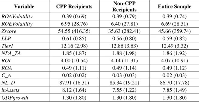
Table 2 contains summary statistics for variables in equation 3 reporting means with standard deviations in parentheses for variables in the CPP recipients subsample, the non-CPP recipients subsample, and the entire sample.
Table 2: Summary statistics reporting means with standard deviations in parentheses.
Table 3 contains results for the fixed effect regressions for all risk measures.
Variable CPP Recipients Non-CPP
Recipients Entire Sample ROAVolatility 0.39 (0.69) 0.39 (0.79) 0.39 (0.74) ROEVolatility 6.95 (28.76) 6.40 (27.81) 6.69 (28.31) Zscore 54.55 (416.35) 35.63 (282.41) 45.66 (359.74) LLP 0.61 (0.85) 0.56 (0.80) 0.59 (0.82) Tier1 12.16 (2.98) 12.86 (3.63) 12.49 (3.32) NPA_TA 1.85 (1.87) 1.88 (1.98) 1.86 (1.92) ROI 4.00 (10.54) 4.14 (11.31) 4.07 (10.91) ROA 0.49 (1.11) 0.49 (1.14) 0.49 (1.12) C_A 0.02 (0.02) 0.03 (0.03) 0.02 (0.03) NL_D 87.91 (16.31) 85.34 (19.21) 86.70 (17.78) lnAssets 8.12 (1.64) 7.55 (1.22) 7.85 (1.49) GDPgrowth 1.30 (1.80) 1.30 (1.80) 1.30 (1.80)
Table 3: Fixed effect panel regression results—all risk measures.
Bank and year fixed effects, robust standard errors reported in parentheses.
Significance levels at 10%, 5%, and 1% are indicated by *, **, and ***, respectively.
CPP Recipients: 149 cross-sections, 2006-2013. 1192 observations. Non-CPP Recipients: 132 cross-sections, 2006-2013. 1056 observations.
ROA Volatility ROE Volatility Z-score Loan Loss Provisions to Total
Assets Variable CPP Recipients Non-CPP Recipients CPP Recipients Non-CPP Recipients CPP Recipients Non-CPP Recipients CPP Recipients Non-CPP Recipients AfterCPP 0.1781** (0.0772) 0.2406** (0.1069) 5.9931* (3.2961) -3.2958 (3.5592) 51.0792 (44.0949) 85.2512 (87.7692) 0.1876* (0.0970) 0.1663** (0.0792) AfterCPP*Thrift -0.1245** (0.0507) 0.0243 (0.0804) -3.8429** (1.7720) -3.6130 (3.6451) -212.6263 (157.8560) 6.1103 (20.5893) 0.1559* (0.0853) 0.1481 (0.1101) Tier1 0.0155 (0.0103) 0.0237** (0.0106) -0.8134 (0.6634) -0.3809 (0.5625) -1.1510 (4.2382) -2.6729 (3.0505) 0.0125 (0.0107) -0.0141** (0.0071) NPA_TA 0.0169 (0.0188) -0.0157 (0.0212) 2.8385 (2.4669) 3.7808 (2.8754) 3.2899 (4.9291) -11.3060* (5.8742) 0.0391 (0.0270) 0.0299 (0.0276) ROI 0.0120 (0.0106) 0.0152 (0.0242) -1.2906* (0.7225) -3.2649** (1.4912) 5.5947 (5.9475) -0.4435 (0.7394) 0.0147 (0.0129) -0.0304** (0.0136) ROA -0.0338*** (0.1157) -0.4653* (0.2746) 7.4887 (7.4390) 23.0009* (12.4840) -32.0655 (44.1522) 3.6630 (7.7680) -0.3049** (0.1260) 0.1248 (0.1320) C_A 2.4484 (2.2870) 0.7022 (1.1567) -16.4322 (56.3489) 110.0699 (95.3812) 1721.4990 (1219.2970) -186.7039 (171.2594) 0.0806 (0.8640) 0.8597 (0.7918) NL_D -0.0016 (0.0027) 0.0005 (0.0029) -0.1742 (0.1410) -0.0137 (0.0875) 2.2409** (1.0513) 0.9801 (0.8581) -0.0046 (0.0029) -0.0016 (0.0019) lnAssets -0.3562*** (0.1288) -0.4382*** (0.1576) -20.4132 (13.5401) -6.0216* (3.5477) -2.4616 (39.6206) -28.1109 (29.0156) -0.3102** (0.1412) -0.0583 (0.1059) GDPgrowth -0.0337*** (0.0121) -0.0030 (0.0132) 0.5527 (0.7453) 0.6616 (0.8780) 10.3466** (4.2950) 12.6197 (13.1424) -0.1394*** (0.0211) -0.1109*** (0.0182) Constant 3.1571*** (1.1645) 3.3339*** (1.0865) 188.8338 (121.7104) 52.0019 (32.4297) -188.3121 (285.7662) 176.6291 (145.4332) 3.4116*** (1.2922) 1.2782* (0.7653) Prob > F 0.0000 0.0000 0.0000 0.0000 0.0074 0.0007 0.0000 0.0000 R2 (within) 0.2640 0.2703 0.1554 0.3617 0.0242 0.0136 0.3898 0.3725
The variable AfterCPP has a significant positive effect on ROA volatility within both subsamples, with both estimates significant at the 5% level. This indicates that CPP recipients and non-CPP recipients both experienced increases in ROA volatility following the
implementation of CPP. These findings differ from those of Duchin and Sosyura (2014), who find an increase in ROA volatility among banks that received CPP after the bailout but do not find this same effect for banks that did not receive CPP funds. Several reasons may explain why the findings of the paper are different. First, this study has the most recent sample of data from the years 2006 to 2013, while their study examines a sample period of 2006 to 2010. Their variable AfterCPP is an indicator that is equal to one during the years 2009 to 2010. It is possible that regressions including more time periods of data are able to capture CPP banks and non-CPP banks’ respective risk returning to levels that are similar to one another several years after the implementation of the bailout, once markets have returned to more stable levels. Another reason why the findings of the paper may differ is because their sample consists of a larger amount of cross-sections, due to their hand collecting of financial data from banks that is unable to be obtained through mediums such as Bloomberg or Compustat. Thus, based on the results from the regression analysis, hypothesis 1 is rejected.
When estimating the equation using ROEVol as the dependent variable, a significant positive coefficient is found for the variable AfterCPP in the CPP recipients subsample but not within the non-CPP recipients subsample. This variable is significant at the 10% level. These findings are supportive of the first hypothesis that banks that received CPP funds will experience greater levels of risk ex-post. These findings are similar to those of Duchin and Sosyura (2014) regarding measures of earning volatility as a representation of risk. A moral hazard effect of CPP on risk is evident within this class of risk. It can be inferred from these results that CPP
recipients have experienced on average an increase of about 6 standard deviations of ROE since the bailout, while banks that did not receive funds are experiencing similar levels of ROE volatility as before the bailout.
When analyzing results when the equation is estimated with Zscore as the dependent variable, it is important to note that the Z-score has an inverse property and an increase in the value of the measure means that a firm is less likely to default, while a decrease in the value of the measure means a firm is more likely to default. Probability of bankruptcy among banks in the sample seems to overall be unaffected by variables of interest within the equation.
Coefficient estimates for the variable AfterCPP are not found to be significant in both
subsamples. While analyzing these results, it does not seem likely that banks that received CPP funding had any major differences in performance regarding the Z-score than banks that did not receive CPP funds, similar to findings regarding ROA volatility. These findings lead to a rejection of the first hypothesis. Duchin and Sosyura (2014) find an increase in probability of default for CPP banks relative to non-CPP banks. This may again be attributable to their smaller time period under analysis.
Significant positive coefficients for AfterCPP within both subsamples when the equation is estimated using LLP as the dependent variable indicates that both CPP recipients and non-CPP recipients experienced increased levels of loan loss provisions following the implementation of CPP. Although banks in both subsamples experienced increases in this measure of risk after the bailout, CPP recipients experienced a higher increase in loan loss provisions to total assets after the bailout than non-CPP recipients. CPP recipients had an increase in LLP of 0.1876% while non-CPP recipients had an increase in LLP of 0.1663%. While these results are similar, CPP recipients still experienced a greater marginal increase than non-CPP recipients. These findings
are once again consistent with hypothesis 1. These findings may be indicative of a moral hazard effect on CPP recipients.
The variable AfterCPP*Thrift yields interesting results when the equation is estimated with ROAVol as the dependent variable. The variable has a significant negative effect on ROA volatility within banks that received CPP funds. This significant effect is not found in banks that did not receive funds. Similar results are found when the equation is estimated with ROEVol as the dependent variable. These findings may indicate that thrift banks that received CPP funds are actually taking less risk within their investment portfolios in comparison to before the bailout and crisis. It is possible that thrift banks that received CPP were the most risky before the crisis, and they are now recognizing that operations before the bailout such as bundling mortgages may not be within their best interest in the future. Coefficient estimates for the variable
AfterCPP*Thrift within equations with ROEVol and ROAVol as the dependent variable leads to a rejection of hypothesis 2.
When the equation is estimated with LLP as the dependent variable, the coefficient for the variable AfterCPP*Thrift is once again significant for CPP recipients but insignificant for non-CPP recipients. In this case the coefficient is positive. Original intuition is that thrift banks that received CPP funds are operating more riskily than they did before they received the funds. These results contrast with those found when the equation was estimated with ROE volatility and ROA volatility as the dependent variable. In these two regressions, the coefficient was negative, suggesting that thrift banks that received CPP funds have decreased their respective levels of risk.
A deeper analysis of how loan loss provisions to total assets is measured shows that these findings may be in fact consistent with those in other regressions. Loan loss provisions is an
expense that a firm is able to calculate before it is actually incurred. For example, a bank may issue a month loan where it expects to have the loan paid back in full by the end of the 12-month period. If after 6 12-months, the firm believes that the borrower may default, it can calculate a provision for this loan, which creates an expense for the estimated loss. It is possible that this increase in loan loss provision expense after the bailout among thrift banks that received CPP funds may be a result of these firms being more cognizant of the amount of risk that mortgage securities possess. As stated earlier in this paper, mortgage securities were not properly rated and their true default risk was not completely realized. Banks that were hit hardest by the mortgage crisis were also most likely banks that sought help through CPP. It is possible that these banks are taking a more conservative approach in evaluating the default risk of their respective securities.
Significant coefficients for control variables that are consistent across subsamples and risk measures follow intuition. Negative coefficients for ROI show that the greater is a bank’s return on investment, the less earnings volatility and loan loss provision expense it will experience. Negative coefficients for lnAssets show that banks with a greater amount of total assets have less earnings volatility. Negative coefficients for the variable GDPgrowth indicate that when the economy is in a state of improvement, earnings volatility is lower, probability of default decreases, and the amount of loans a firm estimates to lose in a given period is reduced.
VII. Conclusion
The purpose of this analysis was to examine the effect that the Capital Purchase Program had on bank risk following the implementation of the program, and to determine if this effect on risk is different among banks with different operational structures. This paper contributes to the
literature by analyzing how the effect on risk differs among banks with different operational structures, and by extending the sample period from previous studies. Findings that differ between firms that received CPP funds and those that did not indicate that firms that received funds have since increased ROE volatility and have also experienced a greater increase in the ratio of loan loss provisions to total assets. Decreases in risk and an increase in risk transparency were found after the capital infusion among thrift banks that received CPP.
Several implications arise from this analysis. This study should be of interest to policymakers within banking regulation institutions. These institutions should take into consideration the possibility that increases in risk measures among CPP recipients may be a result of a moral hazard effect. Other implications arise from findings relative to thrift banks. It is evident that thrift banks are not partaking in similar actions as before the crisis and bailout, thus a future financial crisis caused by these banks’ operations may be less likely.
Certain limitations exist in this study. Future research should address these limitations by using more complex calculations of risk in order to capture more specific changes in risk levels. New default risk measures have been recently developed which use a more statistical approach in calculation, rather than simple ratios or measures of volatility. Using these new measures may reveal other interesting findings and have important implications. Future research may also be concerned with how firms that received funding through more than one investment program have reacted differently than those that have only received funding through one program. As more current data becomes available, future research should also extend the number of years under analysis, in order to monitor and realize how firms that received funding are behaving up to the most recent point in time.
VIII. References
Acharya, Viral V., and Yorulmazer Tanju. 2006. Too Many to Fail—An Analysis of Time-Inconsistency in Bank Closure Policies. Journal of Financial Intermediation 16 (September): 1-31.
Altman, Edward. 1968. Financial Ratios, Discriminant Analysis, and the Prediction of Corporate Bankruptcy. The Journal of Finance 23 (September): 589-609.
Bayazitova, Dinara, and Shivdasani, Anil. 2012. Assessing TARP. The Review of Financial Studies 25: 377-407.
Berger, Allen N., Bouwman, Christa H. S., Kick, Thomas, and Schaeck, Klaus. 2014. Bank Risk Taking and Liquidity Creation Following Regulatory Interventions and Capital Support. University of Pennsylvania.
Black, Lamont, and Hazelwood, Lieu. 2012. The Effect of TARP on Bank Risk-Taking. Board of Governors of the Federal Reserve System: International Finance Discussion (March). Corbett, Jenny, and Mitchell, Janet. 2000. Banking Crises and Bank Rescues: The Effect of
Reputation. Journal of Money, Credit and Banking 32 (August): 474-512.
Cornett, Marcia, Li, Lei, and Tehranian, Hassan. The Performance of Banks Around the Receipt and Repayment of TARP Funds: Over-Achievers versus Under-Achievers. Journal of Banking and Finance 37 (November): 730-746.
Coval, Joshua, Jurek, Jakub, and Stafford, Erik. 2008. Forthcoming. The Economics of Structured Finance. Harvard Business School Finance Working Paper 09-060.
Coval, Joshua, and Moskowitz, Tobias. 2001. The Geography of Investment: Informed Trading and Asset Prices. Journal of Political Economy 109: 811-841.
Dam, Lammertjan, and Koetter, Michael. 2011. Bank Bailouts, Interventions, and Moral Hazard.
Deutsche Bundesbank Discussion Paper 10.
Degryse, Hans, and Ongena, Steven. 2005. Distance, Lending Relationships, and Competition.
Journal of Finance 60: 231-266.
Dell ’Ariccia, Giovanni, and Ratnovski, Lev. 2012. Bailouts, Contagion, and Moral Hazard.
International Monetary Fund (February).
Di Iasio, Giovanni, and Perobon, Federico. 2013. Shadow Banking, Sovereign Risk, and Bailout Moral Hazard. Bank of Italy (February).
Duchin, Ran, and Sosyura, Denis. 2014. Safer Ratios, Riskier Portfolios: Banks’ Response to Government Aid. Journal of Financial Economics 113 (July): 1-28.
Ehrenberg, Ronald G., and Oaxaca, Ronald L. 1976. Unemployment Insurance, Duration of Unemployment, and Subsequent Wage Gain. American Economic Association 66 (December): 754-766.
Faccio, Mara, Masulis, Ronald, and McConnell, John J. 2006. Political Connections and Corporate Bailouts. The Journal of Finance 61 (January): 2597-2635.
Haldane, Andrew, and Scheibe, Jorg. 2004. Forthcoming. IMF Lending and Creditor Moral Hazard. Bank of England.
Harris, Oneil, Huerta, Daniel, and Ngo Thanh. 2012. The Impact of TARP On Bank Efficiency.
Journal of International Financial Markets, Institutions, & Money 24 (December): 85-104.
Hau, Harald. 2001. Location Matters: An Examination of Trading Profits. Journal of Finance 56: 1959-1983.
Kedia, Simi, and Rajgopal, Shiva. Do the SEC’s Enforcement Preferences affect Corporate Misconduct? Journal of Accounting and Economics 51 (April): 259-278.
Keeley, Michael. 1990. Deposit Insurance, Risk, and Market Power in Banking. American Economic Review 80 (December): 1183-1200.
Kim, Yunjeen. 2013. Bank Bailouts and Moral Hazard? Evidence from Banks’ Investment and Financing Decisions. University of Rochester.
Kling, Arnold. 2009. Not What they Had in Mind: A History of Policies that Produced the Financial Crisis of 2008. Mercatus Center.
Kohler, Matthias. 2012. Which Banks are More Risky? The Impact of Loan Growth and Business Model on Bank Risk-Taking. Deutsche Bundesbank Research Centre Discussion Paper 33 (November).
Li, Lei. 2013. Tarp Funds Distribution and Bank Loan Supply. Journal of Finance and Banking
37 (December): 4777-4792.
Markovitz, Harry. 1952. Portfolio Selection. The Journal of Finance 7 (March): 77-91.
Mihai, Simona Y. 2011. Bank Bailouts: Lessons to Learn When Patience Is a Virtue. EuroMed Journal of Business 6: 192-205.
Merton, Robert. 1977. On the Cost of Deposit Insurance When There Are Surveillance Costs.
Puddu, Steffano, and Waelchli, Andreas. 2011. Forthcoming. Too TAF towards the risk. University of Neuchatel Institute of Economic Research.
Shehzad, Choudhry, Scholtens, Bert, and Haan Jakob. 2009. Financial Crises and Bank Earnings Volatility: The Role of Bank Size and Market Concentration. University of Groningen. Topel, Robert. 1983. On Layoffs and Unemployment Insurance. The American Economic
Review 73: 541-559.
Wooldridge, Jeffrey. 2002. Econometric Analysis of Cross Section and Panel Data. MIT Press. Wright, Randall. 1991. The Labor Market Implications of Unemployment Insurance and
IX. Appendix A
Table A.1: Hausman-Taylor tests for fixed vs. random effects
Table A.2: First Stage Probit ModelResults
Variable Estimate Standard Error P-value
Miles -0.0001 0.0002 0.699 BlueState 0.0423 0.5613 0.940 Tier1 -0.0234 0.0749 0.755 NPA_TA 0.0111 0.1308 0.933 ROI -0.0009 0.0756 0.991 ROA 0.0162 0.7368 0.982 C_A -0.3264 9.6163 0.973 NL_D 0.0050 0.0133 0.707 lnAssets 0.3385 0.2170 0.119 GDPgrowth 0.0108 0.1259 0.931 constant -2.6114 2.4901 0.294 Wald Chi-squared 2.77 Prob > Chi-squared 0.9863
Significance levels at 10%, 5%, and 1% are indicated by *, **, and ***, respectively. 281 cross sections, 2006-2013. 2,248 observations.
H0: difference in coefficients not systematic
Regression Dependent
Variable Chi-Squared Statistic Prob > Chi-Squared
ROAVol 161.36 0.0000
ROEVol 26.33 0.0033
Zscore 10.99 0.2766
Table A.3: Second Stage Results
Bank and year fixed effects, robust standard errors reported in parentheses.
Significance levels at 10%, 5%, and 1% are indicated by *, **, and ***, respectively. 281 cross sections, 2006-2013. 2,248 observations
Variable ROA Volatility ROE Volatility Z-score Loan Loss Provisions
to Total Assets AfterCPP*𝐶𝑃𝑃̂ -0.0189 (0.0479) 2.1048 (1.4966) -11.5295 (16.8273) 0.0261 (0.0418) AfterCPP* 𝐶𝑃𝑃̂*Thrift -0.1395* (0.0843) -4.1371 (2.9127) -306.1515 (259.0569) 0.3198* (0.1776) Tier1 0.0198*** (0.0070) -0.5203 (0.4471) -2.8541 (2.4981) -0.0006 (0.0063) NPA/TA 0.0054 (0.0144) 3.1784* (1.8676) -2.2779 (3.8925) 0.0314 (0.0190) ROI 0.0132 (0.0133) -2.3270** (0.9939) 2.5888 (3.0009) -0.0084 (0.0118) ROA -0.3969*** (0.1517) 15.4723* (8.5078) -15.3833 (23.5248) -0.0896 (0.1067) C/A 1.3585 (1.1151) 60.7521 (61.3207) 550.7943 (529.3302) 0.4544 (0.5728) NL/D -0.0004 (0.0021) -0.0770 (0.0740) 1.3167** (0.6409) -0.0028* (0.0016) lnAssets -0.3751*** (0.1026) -13.8961** (6.8369) 0.1021 (29.2171) -0.2012** (0.0931) GDPgrowth -0.0531*** (0.0100) 0.5145 (0.8428) 2.1205 (3.8741) -0.1629*** (0.0156) Constant 3.1752*** (0.8002) 121.5565** (58.1257) -50.7669 (205.4911) 2.5116*** (0.7664) Prob > F 0.0000 0.0000 0.0051 0.0000 R2 (within) 0.2609 0.2362 0.0173 0.3718