Applications of Support
Vector-Based Learning
Róbert Ormándi
The supervisors are
Prof. János Csirik
and
Dr. Márk Jelasity
Research Group on Artificial Intelligence of the University of Szeged
and the Hungarian Academy of Sciences
PhD School in Computer Science
University of Szeged
A thesis submitted for the degree of
Doctor of Philosophy
Szeged
2013
An increasing amount of data is stored in electronic form. This phenomenon increases the need of the methods that help to access the useful pieces of in-formation that are hidden in ocean of the collected data. That is, methods to perform automated data processing are needed. The role of machine learning is to provide methods that support this progress, i.e. it provides algorithms that can automatically discover those hidden and non-trivial patterns in data that are useful for us.
In the focus of this thesis stands a special family of machine learning al-gorithms referred to as support vector-based learners. These algorithms are all based on the so-called maximal margin heuristic, which helps to select the fi-nal model from the suitable ones preserving the generalization ability of the model. These methods are quite general, and they have a numerous amazing properties like generalization capability or robustness to noisy data. However, to apply them to a specific task it is needed to adapt them to that particu-lar task. This is challenging since the inappropriate adaptation can result in a drastic decrease in prediction performance or in the generalization capabil-ity; or cause a computationally infeasible situation (e.g. huge computational complexity or untreatable network load in a distributed setting).
ii
various support vector-based learning methods in numerous learning tasks and environments. During this, novel techniques and ideas, which are less frequent or maybe surprising, are investigated and discussed. The consid-ered tasks themselves touch a wide range problems like time series forecast-ing, opinion minforecast-ing, collaborative filterforecast-ing, and the common binary classifica-tion problem. An uncommon computaclassifica-tional environment is also concerned, namely the fully distributed environment.
In the last few year, numerous people had a positive effect on me to finish this thesis. Probably I will not be able to thank all of them directly, but here I try to emphasize some of them.
First of all I would like to express my thanks to my supervisors, Prof. János Csirik and Dr. Márk Jelasity, for their guidance, continuous inspiration on my research and additionally for letting me work in the Research Group on Artificial Intelligence of the University of Szeged and the Hungarian Academy of Sciences. They showed me interesting, yet undiscovered fields and taught me how I can tackle with them applying scientific mentality and knowledge.
I also would like to thank my colleagues and friends for their continuous support. They definitely helped me discover new ideas and made my pe-riod of PhD studies really pleasurable. They are listed in alphabetical order: András Bánhalmi, Róbert Busa-Fekete, Kornél Csernai, Richárd Farkas, István Heged˝us and György Szarvas. Additionally, I would like to thank David P. Curley and Veronika Vincze for correcting this thesis from a linguistic point of view. Moreover, I would like to thank István Heged˝us and Tamás Vinkó for reviewing this thesis.
Last, but not least I would like to thank my wife, Ildikó, for her endless love, support, and inspiration. She kept the home fire burning while I was
iv
working on this thesis. I would like to dedicate this thesis to her and our son, Márk, for expressing my appreciation.
2.1 Skeleton of NEWSCAST and T-MANprotocols . . . 14
2.2 The NEWSCASTprotocol . . . 15
2.3 The T-MAN protocol . . . 16
4.4 Domain Mapping Learner (DML) . . . 39
5.5 Random Nodes based Overlay Management . . . 66
6.6 P2P Stochastic Gradient Descent Algorithm . . . 80
6.7 P2Pegasos . . . 81
6.8 P2Pegasos prediction procedures . . . 82
7.9 Generalized Gossip Learning Scheme . . . 95
7.10 CREATEMODEL: three implementations . . . 97
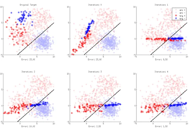
4.1 The first 4 iterations of POLYDML algorithm on Synthetic Database
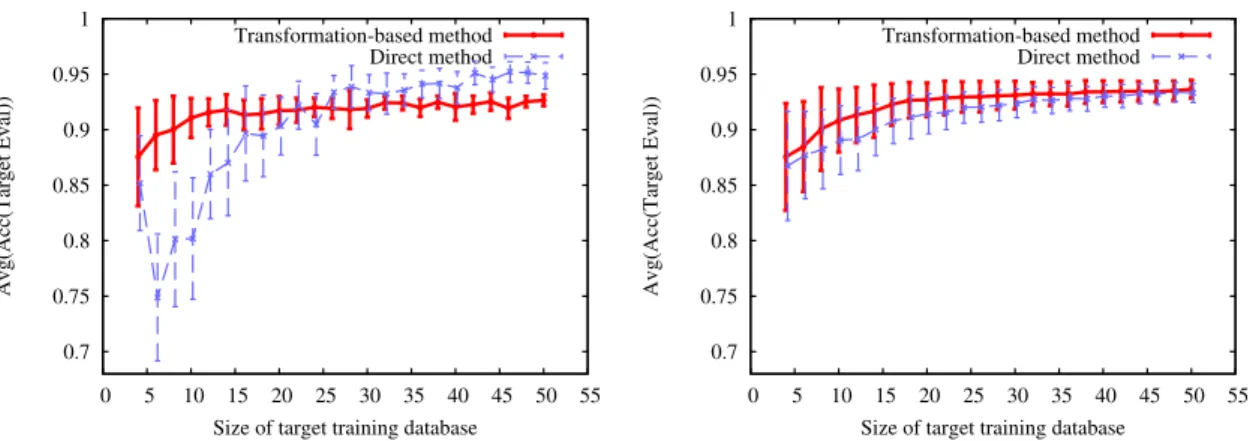
applying linear kernel. . . 44 4.2 The average accuracies and variances of the RBFDML (left) and
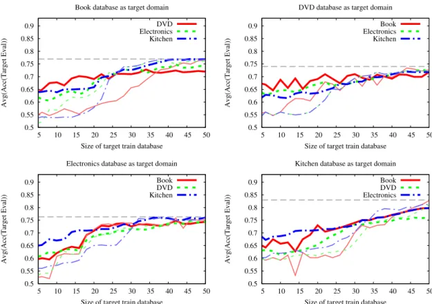
LRDML (right) algorithms using different sizes of subsets of the target domain of synthetic database. . . 45 4.3 The average accuracies of RBFDML algorithm using different
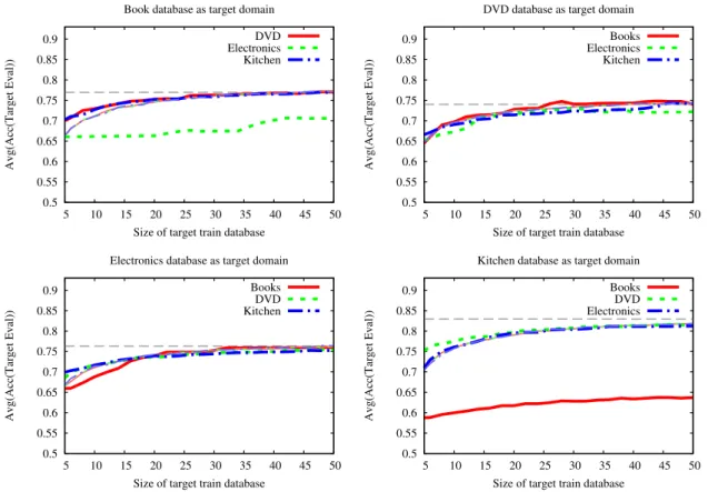
sizes of subsets of the target domains of Multi-Domain Senti-ment Dataset. . . 46 4.4 The average accuracies of LRDML algorithm using different
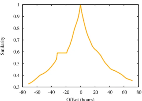
sizes of subsets of the target domains of Multi-Domain Senti-ment Dataset. . . 47 5.1 Sparsity changes during trace interval. . . 58 5.2 Similarity as a function of time. . . 58 5.3 F-measure scores of the different time-shift datasets for positive
(1) and negative (0) ratings against the result on the file owner-ship dataset. . . 61 5.4 The mean absolute error (MAE) of the SMO, J48, LogReg and
viii
5.5 In-degree distribution of the benchmark datasets. . . 64 5.6 Effect of parameterrin a few settings. . . 70 5.7 Experimental results. The scale of the plots on the right is
loga-rithmic. . . 71 5.8 Effect of adding randomness to the view. Thin horizontal lines
show then=0 case. . . 72 6.1 Experimental results over the Iris databases. . . 86 6.2 Experimental results over the large databases, and the Iris1 database.
Labels marked with a ‘V’ are variants that use voting. . . 88 7.1 Experimental results without failure (left column) and with
ex-treme failure (right column). AF means all possible failures are modeled. . . 109 7.2 Prediction error (left column) and model similarity (right
col-umn) withPERFECT MATCHING and P2PEGASOSUM. . . 110
7.3 Experimental results applying local voting without failure (left column) and with extreme failure (right column). . . 111
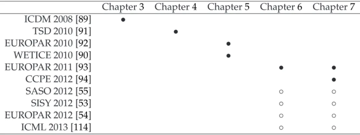
1.1 The relation between the chapters of the thesis and the referred publications (• denotes thebasic publications, while◦ refers to
related publications). . . 3
3.1 MSEs of forecasting of various configurations of the LS-SVM and VMLS-SVM methods on the 100 missing values. . . 28
3.2 Comparison between the main methods on CATS benchmark. . 29
3.3 SMAPE of each time series using the VMLS-SVM andǫ-insensitive SVM regression methods. . . 30
3.4 Comparison between the methods on Santa Fe D data set. . . . 32
5.1 Online session interpolation rules. . . 57
5.2 Offline session interpolation rules. . . 57
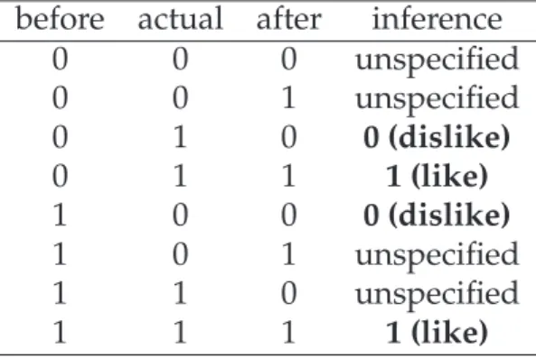
5.3 Rating conversion rules. . . 59
5.4 Basic statistics of datasets. . . 63
6.1 The main properties of the data sets, and the prediction error of the baseline sequential algorithms. . . 83
List of Figures vii List of Tables ix Contents xi 1 Introduction 1 2 Background 5 2.1 Supervised Learning . . . 6
2.1.1 Support Vector Machine . . . 7
2.2 Fully Distributed Systems . . . 12
2.2.1 Overlay Management . . . 14
3 VMLS-SVM for Time Series Forecasting 19 3.1 Related Work and Background . . . 20
3.2 VMLS-SVM . . . 22
3.2.1 How Our Method Is Applied to Time Series Forecasting 25 3.3 Experimental Results . . . 25
xii
3.3.2 Results on CATS Benchmark . . . 27
3.3.3 Results on the Dataset of NN3 Neural Forecasting Com-petition . . . 29
3.3.4 Results on the Santa Fe Data Set D . . . 31
3.4 Conclusions . . . 32
4 Transformation-based Domain Adaptation 33 4.1 Related Work . . . 34
4.2 Transformation-based Domain Adaptation Approach . . . 35
4.2.1 Domain Adaptation Task . . . 35
4.2.2 Transformation-based Approach . . . 36
4.2.3 Transformation-based Approach Based on Linear Trans-formation . . . 37
4.2.4 Support Vector Machine as Source Model . . . 38
4.2.5 Logistic Regression as Source Model . . . 41
4.3 Experimental Results . . . 42
4.3.1 Evaluation Methodology . . . 42
4.3.2 Synthetic Database . . . 43
4.3.3 Results on the Multi-Domain Sentiment Dataset . . . 45
4.4 Conclusions . . . 49
5 SVM Supported Distributed Recommendation 51 5.1 Related Work . . . 52
5.2 Inferring Ratings from Implicit User Feedbacks . . . 55
5.2.1 Filelist.org Trace . . . 55
5.2.2 Inferring Ratings from the Trace . . . 56
5.2.3 Evaluation . . . 59
5.3 Interesting Properties of CF Datasets . . . 62
5.4 Algorithms . . . 65
5.4.1 BUDDYCAST based Recommendation . . . 65
5.4.2 kNN Graph from Random Samples . . . 66
5.4.3 kNN Graph by T-MAN . . . 67
5.4.4 Randomness Is Sometimes Better . . . 68
5.6 Conclusions . . . 73
6 P2PEGASOS—A Fully Distributed SVM 75 6.1 System and Data Model . . . 76
6.2 Background . . . 77 6.3 Related Work . . . 78 6.4 The Algorithm . . . 80 6.5 Experimental Results . . . 82 6.5.1 Experimental Setup . . . 83 6.5.2 Results . . . 85 6.6 Conclusions . . . 88
7 Speeding Up the Convergence ofP2PEGASOS 91 7.1 Fully Distributed Data . . . 93
7.2 Background and Related Work . . . 94
7.3 Gossip Learning: the Basic Idea . . . 95
7.4 Merging Linear Models through Averaging . . . 98
7.4.1 The Adaline Perceptron . . . 99
7.4.2 Pegasos . . . 101
7.5 Experimental Results . . . 105
7.5.1 Experimental Setup . . . 105
7.5.2 Results and Discussion . . . 108
7.6 Conclusions . . . 112
8 Summary 115 8.1 Summary in English . . . 115
8.1.1 VMLS-SVM for Time Series Forecasting . . . 116
8.1.2 Transformation-based Domain Adaptation . . . 117
8.1.3 SVM Supported Distributed Recommendation . . . 118
8.1.4 P2PEGASOS—A Fully Distributed SVM . . . 119
8.1.5 Speeding Up the Convergence of P2PEGASOS . . . 120
8.2 Summary in Hungarian . . . 121
8.2.1 VMLS-SVM id˝osorelemzésre . . . 121
xiv
8.2.3 SVM-mel támogatott elosztott ajánlás . . . 122 8.2.4 P2PEGASOS—Egy teljesen elosztott SVM . . . 123
8.2.5 A P2PEGASOS konvergenciájának további gyorsítása . . 124
Introduction
More and more data is accumulated around us. The year 2012 was called the year of “big data” meaning that various tools become easily available for man-aging very large-scale data, while the storage of data is getting cheaper and cheaper. This phenomenon—although the problem of machine learning has long been considered fundamental—continuously increases the need for ma-chine learning algorithms that workproperlyon specific tasks, and operate ef-ficientlyin unusual settings (like in distributed computational environments), since without these algorithms we simply cannot extract useful information from the data. That is, without the appropriate application of machine learn-ing algorithms, we are not able to utilize that large amount of data. However, achieving these goals is still challenging, since the inappropriate adaptation of a learning algorithm to a specific task can yield models that are far from the optimal ones. On the other hand, the naive adaptation of the algorithms can result in unexpected effects within the system that applies them (like huge, unbalanced load in a distributed system).
The aim of this thesis is to present various approaches which help achieve these goals (appropriate adaptation of the algorithms in terms of both
algorith-2
mic and system aspects) related to a specific learning algorithm family, referred to assupport vector-based learners1. That is, we investigate theadaptivityof sup-port vector-based learners to various tasks and computational environments. The main “take-home message” of the thesis can be summarized as follows. One can achieve significant improvements through applying powerful basic ideas, like the maximal margin heuristic of support vector-based learners, as building-blocks, and careful system design.
The thesis starts with an introductory chapter (Chapter 2), which sum-marizes the necessary background information related to support vector ma-chines and fully distributed systems.
The main part of the thesis can roughly be divided into two distinct parts. In the first part (Chapters3-5), we investigate thealgorithmic adaptivityof sup-port vector machines. That is, we focus on how we can adapt the basic idea of support vector-based learners, the maximal margin heuristics, to develop ef-ficient algorithms to a wide-range of applications, like time series forecasting (in Chapter3), domain adaptation (in Chapter 4), and recommender systems (in Chapter5). The general work-flow here is that we consider a task, inves-tigate the special aspects of the given problem, propose an algorithm which utilizes the observed characteristics of the problem by applying the maximal margin heuristics, and finally evaluate the algorithm in thorough empirical experiments against the state-of-the-art, and often idealized baselines. During the algorithm design, we take into account the computational efficiency, and other practical aspects of the proposed algorithms to get a practical result.
Chapter3 provides an extension for the Least Square Support Vector Ma-chine, which is more suitable for learning time series. After providing the details of the algorithm, the evaluation of the method follows against several baselines on three widely used benchmark datasets.
In Chapter 4, a general domain adaptation mechanism is proposed with two distinct instantiations (one of them is based on support vector machines). Then, the evaluation points out that while both instantiations outperform the baseline methods, the support vector-based approach is a more suitable choice
Table 1.1: The relation between the chapters of the thesis and the referred pub-lications (• denotes the basic publications, while ◦ refers to related publica-tions).
Chapter3 Chapter4 Chapter5 Chapter6 Chapter7
ICDM 2008 [89] • TSD 2010 [91] • EUROPAR 2010 [92] • WETICE 2010 [90] • EUROPAR 2011 [93] • • CCPE 2012 [94] • SASO 2012 [55] ◦ ◦ SISY 2012 [53] ◦ ◦ EUROPAR 2012 [54] ◦ ◦ ICML 2013 [114] ◦ ◦
from the instantiations.
The next chapter (Chapter5) has a twofold contribution. First, it proposes an unusual use-case of the support vector machine to validate the learnabil-ity of a recommender database generated from implicit user feedback. Sec-ond, it investigates how we can adapt the centralized collaborative filtering approaches in a fully distributed setting. In this way, this chapter relates to both parts of the thesis.
In the second part of the thesis (Chapters5-7), we turn to examine the sys-tem model aspect of adaptivity. In this part, our main question is how we can im-plement support vector-based learning algorithms in a specific system model that is radically different from the usual ones.
In Chapter 6, we carefully define the addressed system model, referred to as fully distributed system model. Then, we propose a gossip-based support vector implementation called P2PEGASOS. The basic idea of the protocol is that
online support vector models take random walks in the network while update themselves using the training samples available in the nodes. The algorithm has some notable properties, like fast convergence speed, applicability of fully distributed data (that is, there is no need to move the data from the nodes of the network), simplicity, and extreme tolerance to various network errors (like message drop and delay).
4
In the following chapter (Chapter7), we improve significantly the P2PEGA -SOS algorithm by introducing a general ensemble learning component which
increases the convergence speed of the algorithm by an order of magnitude while keeps all the original advantages. Here we provide a proof of the con-vergence of the algorithm.
Each chapter of the thesis is based on at least one accepted publication. Tab.1.1shows the relation among the chapters of the thesis and the more im-portant1publications.
1For a complete list of publications, please visit the corresponding section of my website:
Background
This work involves some topics that are based on common results from the field of machine learning and distributed systems. These topics clearly have a crucial role in understanding our results. So, we dedicate this chapter to overview some of the most important concepts from these fields.
In the next sections, we briefly introduce the problem of supervised learn-ing and show the classic way of how the Support Vector Machines [24,31,119] learning algorithm tackles this problem. This overview gives us the key insight to understand the basic concepts of support vector-based learning. Later in this chapter, we turn to discuss the basics of the fully distributed systems. Here, we briefly overview the concept of overlay networks and describe two particular unstructured overlay network management protocols, called NEWSCAST [64],
and T-MAN [63], respectively, which are used intensively in the later chapters
of the thesis.
We want to emphasize that the results described here have been achieved by others.
2.1. SUPERVISED LEARNING
6
2.1 Supervised Learning
Let us assume that we are given a labeled database in the form of pairs of fea-ture vectors and their correct labels, i.e. D = {(x1,y1), . . . ,(xn,yn)}, where
xi ∈ Rd and yi ∈ L. The constant d is the dimension of the problem (the number of features) andL denotes the set of labels. We distinguish between
supervised regression problem and classification problem. When the range of labels is continuous e.g. L = R, we talk about regression. However, when it
is discrete and finite, i.e. L= {C1, . . . ,Cl}, we refer to the problem as
classifi-cation where the number of classes isl. The special case of classification when the number of possible class labels equals to two is called binary classification problem. In this case we assume that—without the loss of generality—the set of labels is L = {−1,+1}. Slightly different learning algorithms can be
ap-plied for regression and classification, but the goal is similar in the case of both problems.
The main goal ofsupervised learning(including classification and regression) can be defined as follows. We are looking for amodel f : Rd →Lthat correctly
predicts the labels of the available feature vectors, and that can also general-ize well; that is, which can predict unseen examples too. The generalization property of the model is crucial since a trained model is mainly used for pre-dicting of unseen examples. To be able to achieve generalization it is assumed that the unseen examples come from the same probability distribution than those were used for training. This is one of the main assumptions of machine learning [84].
During the training phase, a supervised learning algorithm seeks for a suit-able model from a predefined (by the training algorithm itself) model space called hypothesis space. This phase can be thought of as an optimization pro-cess, where we want to maximize prediction performance, which can be mea-sured via, e.g. the number of feature vectors that are classified correctly over the training set. The search space of this problem is the hypothesis space and each method also defines a specific search algorithm that eventually selects one model from this space keeping in mind the preservation of the generalization property of the model.
Training algorithms that process the training database as a continuous stream of training samples (i.e. stream of(xi,yi)pairs) and evolve a model by updat-ing it for each individual trainupdat-ing sample accordupdat-ing to some update rule are calledonline learning algorithms. These algorithms are often used in large scale learning problems [78], there is no need for storing the whole training database in the memory.
In various machine learning tasks, the available training data is often par-titioned into a training set and an evaluation set. In this case we assume that during the training phase the algorithm accesses only to the training set and the evaluation set is completely hidden.
2.1.1 Support Vector Machine
In the previous section, we introduced the main concepts of the supervised learning. Here we discuss a particular supervised learning algorithm family— namely the family of Support Vector Machines (SVMs) [24, 31, 119]—which plays a central role in this work.
The name SVM or more generally support vector-based learning refers to a supervised learning family instead of a particular algorithm [31]. The al-gorithms belonging to this family were designed around a central idea called maximal margin heuristic. The basic idea of support vector-based learning is pretty simple: find a good learning boundary while maximizing the margin (i.e. the distance between the closest learning samples that correspond to dif-ferent classes). In this way, each algorithm that optimizes an objective func-tion in which the maximal margin heuristic is encoded can be considered a variant of the SVMs. In the following, to show some interesting properties of SVMs, we briefly discuss a particular SVM classification algorithm (and its soft-margin and kernel-based extensions).
Let us assume that we are in a binary classification setting, i.e. we have a setDof training samples containing npairs in the form(xi,yi)wherexi ∈ Rd
andyi ∈ {−1,+1}.
In its simplest form the SVM is expressed as a hyperplane parametrized by the normal vector (that is orthogonal to the hyperplane) of the plane (w ∈Rd)
2.1. SUPERVISED LEARNING
8
and a scalar (b∈ R). Given such a hyperplane the model of the SVM is writtenin the following form:
f(x) =sign(wTx+b). (2.1) The geometrical interpretation of this kind of model is pretty clear: the model assigns label −1 to the inputs that are below the hyperplane and +1 that are above.
During the training phase the SVM seeks for the appropriate parameters that separate the training samples and maximize the margin. Formally it is done by searching in the space of canonical hyperplanes [31] corresponding to the training setD. It is easy to see that a hyperplane with parameters(w,b)is
equally expressed by all pairs of(λw,λb)parameters where 0<λ ∈R. Let us
define a canonical hyperplane to be such that separates the training database correctly with a distance of at least 1, i.e.:
wTxi+b≥1 whenyi = +1,
wTxi+b ≤ −1 whenyi =−1 for each sample 1≤i ≤n (2.2) or in a more compact form:
yi(wTxi+b) ≥1 for each sample 1≤i≤n. (2.3) Given a canonical hyperplane (w,b), we can obtain thegeometrical distance from the plane to a data pointxiby normalizing the magnitude ofw:
dist((w,b),xi) = yi(wTxi+b)
kwk ≥
1
kwk. (2.4)
As one can see, the geometrical distance between the canonical hyperplane
(w,b)and each training pointxican be bounded by the reciprocal of the norm ofw.
The SVM training algorithm wants to maximize the margin, i.e. the geo-metrical distance between the closest training points from the opposite classes in the space of canonical hyperplanes [31]. Given a canonical hyperplane
(w,b)—based on the bound in Eq.2.4—the margin is at least kwk2 i.e. to max-imize it, the training algorithm has to minmax-imize the quantity kwk or equally
1
2kwk2(to get a more handy objective function).
Based on the definition of the canonical hyperplanes and the above ob-served bound on the margin, we can easily formalize the optimization problem of the SVM:
minimizew,b 1 2kwk2
subject to yi(wTxi+b)≥1 (for each 1≤i ≤n).
(2.5) As one can easily notice that the above defined optimization problem is pretty restricted in the sense, it is only defined for separable training sets (be-cause of the concept of canonical hyperplanes). Extending this optimization problem to the so-calledsoft-margin[31] optimization can overcome this prob-lem. To achieve this we introduce a non-negative ξi ∈ R (1 ≤ i ≤ n) slack variable for each condition of the above defined optimization problem. For a given conditioni, this variable models how that condition violates the condi-tion of being a canonical hyperplane, i.e. the error corresponds to be canonical hyperplane. By introducing the slack variables, we tolerate some error in those conditions. However, if we want this error to be as small as possible, we have to extend the objective function as well by adding the slack variables to it. Based on the introduction of slack variables, we get the soft-margin optimiza-tion form of SVM classificaoptimiza-tion:
minimizew,b,ξ 1 2kwk2+C n
∑
i=1 ξisubject to yi(wTxi+b) ≥1−ξiandξi ≥0 (for each 1≤i ≤n). (2.6)
trade-2.1. SUPERVISED LEARNING
10
off between the error minimization and margin maximization.During the SVM training we have to solve the optimization defined in Eq.2.5or Eq.2.6. Now let us focus on the more general soft-margin form. The original form of this optimization problem showed above is calledprimal form. Numerous methods exist that solve the optimization problem in this original form [26]. However in some scenarios (e.g. in centralized computation mod-els), there are some advantages—most importantly, one can apply the kernel-based extension that introduces nonlinearity into the approach [24, 119]—of transforming this form to the so-calleddual form.
The dual form of Eq.2.6is found by first taking the Lagrangian of the opti-mization problem: L(w,b,ξ,α,ν) =1 2kwk2+C n
∑
i=1 ξi − n∑
i=1 αi(yi(wTxi+b)−1+ξi)− n∑
i=1 νiξi αi ≥0 (for each 1≤i≤n) νi ≥0 (for each 1≤i ≤n). (2.7)Then by differentiating with respect to w, b and each element of ξ (i.e.
respect to the non-Lagrangian variables), imposing stationarity, resubstitut-ing the obtained constraints into the primal, and applyresubstitut-ing the Karush-Kuhn-Tucker (KKT) complementary conditions [24, 119], we eventually get the fol-lowing dual form:
maximizeα −12 n
∑
i=1 n∑
j=1 αiαjyiyjxiTxj+ n∑
i=1 αi subject to∑
n i=1αiyi =0 and 0 ≤αi ≤C (for each 1≤i ≤n).
(2.8)
This is a so-called quadratic programming(QP) problem in the variable α ∈
Rn. It is a quite general optimization problem having a unique and globally
solve QP problems [18] and some of them scale well with the size of training database. Nevertheless, the size of this optimization problem is very large (since usually it isn ≫d), which often causes serious problems in practice.
Additionally, from the derivation of the primal equations, it can be seen that the optimal hyperplane can be written as:
w⋆ = n
∑
i=1 α⋆ iyixi b⋆ =1 n n∑
i=1 1−yiw⋆T xi yi (2.9) whereα⋆∈ Rn is the optimal solution of the dual problem. That is, the vector
w⋆ is the linear combination of the training examples [24, 119]. Moreover, it
also can be shown (based on the KKT conditions [119]) that only the closest data points (that are called support vectors) contribute tow⋆ (i.e. have a value α⋆
i > 0). Subsequently, the non-support vectors have a coefficient α
⋆
i = 0 and can be skipped from the model. This leads to the sparse solution [119] of the model: f(x) =sign(
∑
(xi,yi)∈SV α⋆ iyixTi x+b ⋆ ) (2.10)whereSV ⊆Ddenotes the set of support vectors, where usually|SV| ≪ |D|.
The above defined dual representation learns a robust and sparse linear model. But what if the relation between the data and the labels is strictly non-linear? Thekernel representation offers a solution to tackle with the nonlinear-ity by projecting the data into a higher dimensional feature space to increase the representation power of the linear learning machine. That is, we apply a
φ : Rd → Rh nonlinear transformation, whereh ≫ d, to change the
represen-tation of each data pointx∈ Rd.
Mapping the data onto a higher dimensional space each time when we need it would be computationally inefficient. But one can easily recognize that the only way in which the data appears in the training problem in Eq.2.8, and
2.2. FULLY DISTRIBUTED SYSTEMS
12
in the model in Eq.2.10 is in the form of inner products (xiTxj). Now suppose we first transformed the data to the higher dimensional features space, using a mappingφdefined above. Then the training algorithm would only dependon the data through dot products in that feature space, i.e. on functions of the formφ(xi)Tφ(xj). By defining thekernel function K(xi,xj) = φ(xi)Tφ(xj)we can avoid the explicit computation of mappingφ. This procedure is called
kernel-based learning and can increase the representation power of SVMs strictly without significantly increasing the computational complexity. This is why it is pretty often applied together with support vector-base learning algorithms.
Other advantage of the application of kernels is that it can be considered as an external component of the learning which can be modified without modify-ing the learnmodify-ing algorithm itself. Different kernels exist and the construction of the kernels is theoretically well-studied (see e.g. Mercel-theorem [31]). Kernels that are used very often are the polynomial kernel, and the RBF kernel [31], however, kernels for specific tasks exist as well like the alignment kernel (e.g. for time series forecasting), string kernels, and graph kernels [31,33].
The above described variant of SVM deals with classification problems. This model applies a possible formalism of the central idea (margin maximiza-tion) which has extension to the soft-margin optimization to become a more general learning approach, and the kernel-based extension, which is applica-ble to be capaapplica-ble of handling nonlinear relations. However, the basic concept of maximal margin classifiers can be easily formalized in a different way [112] or can be extended to regression problems [31] as well.
2.2 Fully Distributed Systems
In the later part of the thesis, we will move our system model from the tradi-tional random access stored program machine (RASPM) [52]—where you have a single computational unit (CPU), with a central memory—to the so-calledfully distributedenvironments.
These systems are networked environments which contain usually a large number of units, called nodes, that are capable of local computation and can communicate with other nodes using the network. We assume that the
sys-tem consists of a potentially very large number of nodes, typically personal computing devices such as PCs or mobile devices. We do not assume any ho-mogeneity between the nodes. They can be different in their computational power, operating system, or any other characteristics. But we expect that most of them know and run the same protocol (excepting for a few number of mali-cious users, which usually can be tolerated in this type of systems1).
Each node in the system has a unique network address. We assume that a particular node knows the addresses of a constant number of other nodes, called neighbors. The number of neighbors is much less than the size of the network (due to memory limitations), but the set of neighbors can vary in time. If a node A knows the address of node B, we say that node B isconnected to nodeA(connectivity relation).
The communication is done by message passing between connected nodes without any central control (fully distributed aspect). That is, every node can send messages to every other node, provided the address of the target node is available. We assume that messages can have arbitrary delays, and messages can be lost as well (failure scenarios). In addition, nodes can join and leave at any time without warning (churn), thus leaving nodes and crashed nodes are treated identically. Leaving nodes can join again, and while offline, they may retain their state information.
The graph defined by the computational units as nodes, and the connec-tivity relations as edges is called overlay network. The communication is com-pletely based on this graph, since it is a central component of each fully dis-tributed system. The overlay networks are provided by middleware services, called peer sampling services [64]. The peer sampling service is itself a dis-tributed protocol. In the following, we briefly overview two widely used un-structured peer sampling protocols that are used intensively in the later chap-ters.
2.2. FULLY DISTRIBUTED SYSTEMS
14
Algorithm 2.1Skeleton of NEWSCAST and T-MANprotocols 1: n←initNeighbors() 2: loop 3: wait(∆) 4: p ←selectPeer(n) 5: send (n∪currNode()) top 6: end loop
7: procedureONRECEIVENODES(nodes) 8: n ←updateNeighbors(n∪nodes)
9: end procedure
2.2.1 Overlay Management
In Alg.2.1, one can see the basic skeleton of both the NEWSCAST [64] and
T-MAN [63] protocols. The algorithm handles a set ofnode descriptors, stored in
variable n, which contains the addresses (and other node related data) of the nodes known by the current node. The connectivity relations (and so the over-lay itself) is defined by these node descriptor sets. Each node in the network runs the same protocol. Through the run of the protocol, these sets are ex-changed between the nodes to obtain the required overlay network based on local communication.
The algorithm is divided into two distinguished sections: the active behav-ior (left hand side code snippet) and an event handler function (right hand side code snippet;ONRECEIVENODES function). The active behavior consists of an
initialization part and an infinite loop defining periodic activities. The node descriptors are initialized (at line 1 of Alg. 2.1) by applying a node cache or other bootstrap service. The main part of the active behavior consists of a se-quence of periodic activities inside a loop executed in each∆time moment (at
line 3of Alg.2.1). In each active execution, the protocol selects a node stored in its own node descriptor set (at line4of Alg.2.1, based on the abstract
func-tion SELECTPEER). Then, it sends its node descriptor set, extending with its
own descriptor (proposed by the CURRNODE function), to the selected node
(at line5of Alg.2.1).
When a node descriptor set is received, the mechanism defined in the event handle function, calledONRECEIVENODES, is executed. The function takes the
received node set and updates its own set by applying the abstract function
UPDATENEIGHBORS (at line8of Alg.2.1).
informa-Algorithm 2.2The NEWSCASTprotocol 1: procedureSELECTPEER(nodes) 2: node←uniRand(nodes)
3: returnnode
4: end procedure
5: procedureUPDATENEIGHBORS(nodes) 6: nodes ←nodes− {currNode()}
7: s←sortnodes by fieldts
8: returntopK(s)
9: end procedure
10: procedureCURRNODE() 11: d ←initDesc()
12: d.ts ←current time
13: returnd
14: end procedure
tion stored in the node descriptors is not mentioned1, and it contains three
functions that are not yet defined (however, their semantic roles are clearly discussed above).
The NEWSCAST[64] protocol is yielded if one implements the abstract
func-tions as defined in Alg.2.2. Here it is assumed that the node descriptors are extended with a timestamp field, denoted bytsin the pseudo code, containing the time moment when the node descriptor is created by the function CUR -RNODE() (at line 12 of Alg.2.2). In the case of the NEWSCAST protocol, the
update method selects the top-k most freshest node descriptors from the set of received and owned node descriptors providing a continuous sampling of the probably online nodes. The function SELECTPEER supports this behavior
by providing uniform random selection from the available node descriptors. Thus, the NEWSCAST protocol results a dynamic overlay.
The selection of the top-k elements is necessary to avoid the continuous growing of the node sets (at line8of Alg.2.2). This results that the overhead of the protocols consists of sending one message of a constant size to a node periodically. Herekis the parameter of the protocol.
It can be shown that, through the set of node descriptors proposed by the
NEWSCAST protocol, each node can request uniform random samples of the
nodes in the network that are likely to be online at the time of the request [64]. This protocol has been extended to deal with uneven request rates at different
1We assumed earlier only that the address of the node is stored; however, to achieve
2.2. FULLY DISTRIBUTED SYSTEMS
16
Algorithm 2.3The T-MAN protocol 1: procedureSELECTPEER(nodes)
2: node←argmaxo∈nodes(s(currNode(),o))
3: returnnode
4: end procedure
5: procedureUPDATENEIGHBORS(nodes) 6: (nodes ←nodes∪ {rrandom nodes})
7: nodes ←nodes− {currNode()}
8: s←sort nodesbased ons(currNode(), .)
9: returntopK(s)
10: end procedure
11: procedureCURRNODE() 12: d←initDesc()
13: fillCharacteristics(d) 14: returnd
15: end procedure
nodes, as well as uneven distributions of message drop probabilities [116]. For discussing the T-MAN [63] protocol, let us assume that the node
de-scriptors contain the characteristics of the users1that use them, and as : node
descriptor ×node descriptor → R similarity measure is given which can
mea-sure some kind of higher order similarity (e.g. similarity in taste or behavior of users) between two users based on the information that can be found in the node descriptors.
We can obtain the protocol T-MAN by defining the abstract functions of
Alg.2.1in the way given in Alg.2.3. The active behavior of the protocol selects the most similar node (at line2of Alg.2.3) to the current node from the set of node descriptors available locally (through theSELECTPEER implementation).
Through the update, the protocol retains the most similark nodes to the cur-rent node by sorting the incoming nodes based on the functions(currNode(), .)
(at line8of Alg.2.3) varying only in its second argument (as a partially called function, that is, function of one variable). The functionCURRNODEis
respon-sible for creating the node descriptor of the current node. Here the node related characteristics are loaded by the function callFILLCHARACTERISTICSat line13
of Alg.2.3. The details of this function are application dependent, hence we do not discuss it here.
Applying the above mentioned mechanism, this protocol converges to the
1We could say feature vectors of the users if we want to apply the terminology of
similarity overlay of the given measure. That is, an overlay which contains edges to the most similar nodes based on the similarity functions. The speed of the convergence is pretty fast; it is O(log(n)) per node [63]. Considering that the nodes of the network are individual computation units, i.e. this is an asynchronous parallel network, this is a very efficient solution.
The protocol is often extended with an optional modification shown at line 6of Alg. 2.3. Here we add r random node descriptors to the original set making the protocol more explorative. The samples can be provided by e.g.
a NEWSCAST protocol instance which runs on each node separately from the
T-MAN protocol. Hereris another parameter of the protocol.
Numerous other overlay management protocols exist. Here we just high-lighted two of them that are used intensively in the later chapters. For a more detailed description of the above discussed protocols, please read [63,64].
VMLS-SVM for Time Series Forecasting
In the automated data processing thetime dimensionappears very often. Basi-cally each post that we share in the social network sites, each financial trans-action that we execute during each payment, and any activities that are per-formed on the web are stored together with the timestamp when the data was produced. Later this huge amount of time related data is used by data-driven companies to optimize their future revenue by making better decisions related to their business model [45].
The processing of this type of data quite often involves the problem of time series forecasting. Here we want to build statistical models based on the cur-rently available data which make accurate predictions on the future. The appli-cations of these models are almost as diverse as the variety of the related data-sources mentioned above. You can easily find applications in finance where the goal is to predict the changes of the markets, and entertainment where we want to know e.g. how our social network will look like in the near future [66]. However time series forecasting problems are quite common, the appro-aches that deal with it usually come from the field of regression. These mo-dels—however they perform very well in general regression tasks—often lack
3.1. RELATED WORK AND BACKGROUND
20
of those design principles that make really accurate in these type of tasks.For these reasons, in this chapter we propose a novel extension to the Least Squares Support Vector Machines (LS-SVM) [112,113]. This extension, called Variance Minimization LS-SVM (VMLS-SVM) [89], refines the objective func-tion of the original LS-SVM by introducing another parameter. The modifica-tion is based on the preliminary observamodifica-tion that underlines the importance of the variance term of the error function. We describe the theoretical details be-hind the extension, and through a series of empirical evaluation we show that it has a crucial role in solving time series forecasting tasks. We briefly discuss the effect of the new parameter, and show how you can fine-tune it to avoid overfitting.
The results of this chapter are based on our recent work published in [89].
3.1 Related Work and Background
Times series can be modelled by a large class of models which can be roughly divided into two main subclasses, namely linear models and nonlinear ones. The linear models (such as autoregressive (AR) models [19,70], linear regres-sion [29]) have been extensively investigated and are quite advanced, but they only work well when the data dependency is closely linear.
The neural network based regression models can overcome these weak-nesses i.e. they can model nonlinear relations. Both the Artificial Neural Net-works (ANN) [42] and the Radial Basis Function Neural Networks (RBF) [104] are commonly used in time series forecasting. Although they have some in-herent drawbacks, such as the problem of multiple local minima, the choice of number of hidden units, and the danger of overfitting. These problems often make the use of neural network based approaches a bit difficult.
The application of SVMs in regression setting [31] (or SVRs as often re-ferred) can avoid these problems by having unique and globally optimal so-lution [31] and only one hyperparameter (C ∈ R, the margin maximization
trade-off, for more details see Sec.2.1.1, particularly e.g. Eq.2.6). Additionally, they usually achieve a better generalization by applying the margin maximiza-tion technique than the tradimaximiza-tional neural networks. Another advantage of the
SVM approach is the applicability of thekernel-trickwhich makes it more prac-ticable. A slight drawback of training a classical formalized SVM is that it solves a linearly constrained QP problem in the size of training examples, n, which can be huge.
LS-SVM does not have this latter problem. This approach is a reformu-lation of the principles of SVM, which applies equality instead of inequality constraints. Based on this, its solution follows from a linear KKT [112] system instead of a computationally hard QP Problem [24,119].
To give a little insight to the main concept of the LS-SVM formalism, sup-pose that we are in a supervised regression setting and given a training set
D = {(x1,y1), . . . ,(xn,yn)} ⊆ Rd×R. With LS-SVM, one considers the
fol-lowing optimization problem (primal form): minimizew,b,e 1 2kwk 2+ C1 2 n
∑
i=1 e2isubject to yi =wTφ(xi) +b+ei (for each 1≤i ≤n),
(3.1)
whereφ:Rd →Rhis the feature mapping,Cis a trade-off parameter between
generalization and the error minimization, andei ∈ R(0≤i≤n) are the error variables (their roles are similar to the slack variables in the case of classic SVM formalism detailed in Sec.2.1.1).
In the case of LS-SVM the model is given by: f(x) = w⋆T
φ(x) +b⋆, (3.2)
where w⋆
∈ Rh and b⋆
∈ R are the solutions of the optimization problem
defined in Eq.3.1.
The result of the optimization problem is obtained by taking the corre-sponding Lagrange function, differentiating it, and establishing stationarity constraints, which results the following linear equation system:
0 1T 1 Ω+ C1I ! b α ! = 0 y ! , (3.3) where y = (y1, . . . ,yn)T, α = (α1, . . . ,αn)T, 1T = (1, . . . , 1) ∈ R1×n and Ω ∈
3.2. VMLS-SVM
22
Rn×n where Ωi,j = φ(xi)Tφ(x
j) = K(xi,xj) (for each 1 ≤ i,j ≤ n). From the result of the dual problem the optimal solution of the original problem can be computed byw⋆
=∑ni=1αiφ(xi).
This formulation is quite simple and—as one can see above—the method has all of the advantages of SVM, like the applicability of the kernel-trick and it has a unique solution. Moreover, in the case of LS-SVM, the solution comes from solving a linear system of equations, not a quadratic one, which results in an increased efficiency in the computation of the model. But LS-SVM has also one slight drawback. While the classic SVM chooses some samples from the training data (the support vectors) to represent the model (that is, it has a sparse solution shown in Eq.2.9), the LS-SVM uses all the training data to pro-duce the result. Sparseness can also be intropro-duced with LS-SVM by applying a pruning based method to select the most important examples [37,74].
The model is quite general in the sense that it can also be shown to have a connection with regularization networks [41]. When no bias term is used in the LS-SVM formulation, as proposed in Kernel Ridge regression [107], the expression in the dual form corresponds to the Gaussian Processes [123].
3.2 VMLS-SVM
Essentially VMLS-SVM is an extension of LS-SVM, where the objective func-tion of optimizafunc-tion is refined by adding a weighted variance minimizafunc-tion part. The motivation behind this modification is a preliminary observation which can be explained as follows: if two time series forecasting models are given with the same error, usually the better is the one that has a smaller vari-ance, i.e. the one that can produce a smoother fitting. Applying the proposed modification, we can adjust the weight of the variance term of the error func-tion as well with an addifunc-tional hyperparameter.
Now let us describe this method in detail. Suppose that we have a training set D, like that defined in the previous subsection. Next, let us express the
optimization problem of VMLS-SVM in the following way: minimizew,b,e 1 2kwk 2+C1 2 n
∑
i=1 e2i +D1 2 n∑
i=1 ei− 1 n n∑
j=1 ej !2subject to yi =wTφ(xi) +b+ei (for each 1≤i≤n),
(3.4)
where φ, C and ei (1 ≤ i ≤ n) are the same as those of LS-SVM (see Eq. 3.1) and theD parameter is a trade-off between generalization and variance mini-mization. The regression function is the same as before, hence it is defined by Eq.3.2.
As in the case of LS-SVM, the solution of Eq.3.4is obtained from the corre-sponding dual problem:
L(w,b,e,α) =1 2kwk 2+ C1 2 n
∑
i=1 e2i +D1 2 n∑
i=1 ei− 1 n n∑
j=1 ej !2 − n∑
i=1 αiwTφ(xi) +b+ei−yi . (3.5)The optimal solution of this function can be obtained by demanding that the following conditions be satisfied:
∂L(w,b,e,α) ∂w =0→w= n
∑
i=1 αiφ(xi), (3.6) ∂L(w,b,e,α) ∂b =0→ n∑
i=1 αi =0, (3.7) ∂L(w,b,e,α) ∂ei =0→αi = (C+D)ei− D n n∑
j=1 ej for each 1≤i ≤n, (3.8) ∂L(w,b,e,α) ∂αj =0→w Tφ(x j) +b+ej =yj for each 1≤ j≤n. (3.9)From Eq.3.7and3.8we get the following: 0 = n
∑
i=1 αi = (C+D) n∑
i=1 ei−D n∑
j=1 ej =C n∑
i=1 ei. (3.10)3.2. VMLS-SVM
24
This constraint is encoded in the first equation of the final equation system presented in Eq.3.13. The additional constraints can be observed by perform-ing the followperform-ing. For each 1 ≤ j ≤ n, replacingw in Eq. 3.9 with the right hand side of Eq.3.6, and then replacingαi with the right hand side of Eq.3.8.After this manipulation, we get: n
∑
i=1 (C+D)ei−D n n∑
k=1 ek ! K(xi,xj) +b+ej=yj. (3.11)With some additional algebraic manipulation, we arrive at the following: n
∑
i=1 " (C+D)K(xj,xi)− D n n∑
k=1 K(xk,xj) # | {z } Ωj,i ei+b+ej =yj. (3.12)This constraint is encoded in the jth equation (row) of the final equation system shown below in Eq.3.13.
Using Eq. 3.10 and Eqs. 3.12 (for each 1 ≤ j ≤ n) we get the following equation system (these equations do not contain the variables w and α since
they were eliminated):
0 CT 1 Ω+I ! b e ! = 0 y ! , (3.13)
where1, yare the same as in Eq.3.3, CT = (C, . . . ,C) ∈ R1×n, andΩ ∈ Rn×n
where Ωj,i is defined in Eq. 3.12. By solving this equation system, we obtain
the optimal solution of the original optimization problem defined in Eq.3.4. Now the regression function becomes
f(x) = n
∑
i=1 " (C+D)e⋆ i − D n n∑
j=1 e⋆ j # K(xi,x) +b⋆, (3.14) wheree⋆ ∈ Rn, andb⋆∈ Rare the solutions of the equation system shown in
3.2.1 How Our Method Is Applied to Time Series Forecasting
In the above subsection we introduced the details of VMLS-SVM as a regres-sion method. Let us now turn to discuss how we applied this method for modelling time series. A time series is a sequence of vectors,x(t), t = 0, 1, . . . where t represents the elapsed time. For the sake of simplicity, we will con-sider only sequences of scalars here, although each technique can be readily generalised to vector series.
For us, time series forecasting means predicting the value of a variable from a series of observations of that variable up to that time. Usually we have to forecast the value of x(t+k) from the following series of observa-tions: x(t), . . . ,x(t−N+1). Formally this can be stated as: find a function fk : RN → R to obtain an estimate of x at time t+k, from the N time steps
back from timet. Hence for each time momentt
x(t+k) = fk(x(t), . . . ,x(t−N+1)). (3.15) The observations (x(t), . . . ,x(t−N+1))constitute a windowand N is re-ferred to as the window size. The technique which produces all the window-value pairs as training samples for a regression method is called the sliding window technique. This technique slides a window of lengthN+1 over the full time series and generates the training samples in the following form for every possible value ofi:
(xi,yi) = (x(t+i−N+1), . . . ,x(t+i),x(t+i+k)), (3.16) where N−t−1 ≤i,xi ∈ RN, andyi ∈ R. In this way the size of the window
(N) determines the dimension of the regression problem (d).
3.3 Experimental Results
We performed experimental evaluation on several benchmark databases in dif-ferent settings. Before we turn to present our results, we summarize shortly how we performed these evaluations.
3.3. EXPERIMENTAL RESULTS
26
In order to perform time series forecasting using the VMLS-SVM method, we employ the sliding window technique described in the previous subsection which produces an initial training database. Afterwards, our system applies a normalization on the input databases.In our tests, we experimented with three types of kernels for the LS-SVM and VMLS-SVM. These were the following: Polynomial kernel, RBF kernel, Alignment kernel for time series [33]. The first two kernels are general pur-pose, well-known kernels. The last one is especially designed to apply on sequential data like time series. It applies a Dynamic Time Warping based alignment of the samples.
3.3.1 Parameter Selection
As one can see, the VMLS-SVM has two hyperparameters, which makes it more complicated to fine-tune the method and avoid overfitting. Here we de-scribe shortly how we set these parameters.
In our first tests on the first two benchmarks, we applied a simulated an-nealing based [71] optimization method, called parameter optimizer, which optimized the parameters of the underlying learning method. This parame-ter selection method can be viewed as a function minimizing method, where the input of objective function is the parameter of the underlying learner. The value of the function is the aggregated error of the underlying method on a fixed validation set. Of course, the underlying regression method was trained on a different, but also fixed training set using the input of the objective func-tion as parameters. The applied error measure depends on the database eval-uation metric, i.e. it is always the same as the error measure of the evaleval-uation process. The stopping criteria of the parameter selection method was deter-mined by visual inspection, i.e. when the error was quite small and it did not decrease, we stopped the process.
Using this optimization technique, we get a sequence of parameter sets, which was provided by the parameter optimization method. This revealed a trend of a correct parameter setup. Afterwards, we carried out some manually parameterized tests, using experiments from the automatic parameter
selec-tion. These tests were evaluated on the evaluation set, which is completely different from the training and validation sets.
3.3.2 Results on CATS Benchmark
The CATS benchmark [40] is a publicly available database for time series fore-casting. It was made for a competition organized during the IJCNN’04 con-ference in Budapest. This artificial time series has 5,000 data points, among which 100 are missing. The missing values are divided into 5 blocks, elements between 981-1,000, 1,981-2,000, 2,981-3,000, 3,981-4,000, and 4,981- 5,000.
The goal of the competition was to predict these 100 missing values. Twenty-four teams participated and seventeen of them uploaded acceptable predic-tions. The evaluation metric was the mean squared error (MSE) metrics:
MSE= 1 n n
∑
i=1 (yi−yˆi)2, (3.17)computed on the 100 missing values as evaluation set.
In order to make a comparison, we decided to use the LS-SVM and our VMLS-SVM in the same way. We defined twenty different prediction functions based on Eq. 3.15. In this setup the first prediction function (f1) was used to
predict the first missing value, the second prediction function (f2) was used to
predict the second missing value, and so on. Each prediction function used the same parameter setting, which was provided1 by the parameter optimization
method in the early tests. This optimization process used a validation set to test the goodness of different parameter setups. This validation set was gener-ated in the following way: from the end of each training block we split the last 20 values. Afterwards, using the experiments of the automatic parameter opti-mization, we carried out some tests, using the fixed parameterized prediction method. In this phase, for each prediction function we trained its own LS-SVM or VMLS-SVM learner with the same parameter values on the full training set. The overall results are presented in Table3.1.
3.3. EXPERIMENTAL RESULTS
28
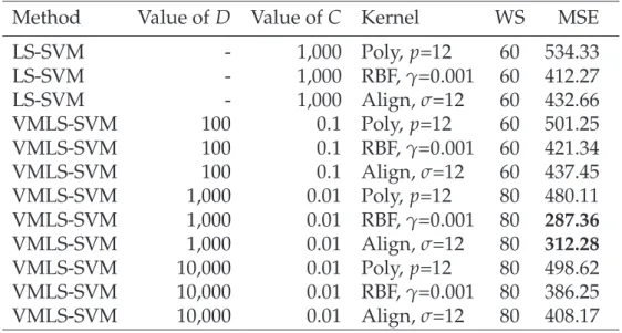
Table 3.1: MSEs of forecasting of various configurations of the LS-SVM and VMLS-SVM methods on the 100 missing values.
Method Value of D Value ofC Kernel WS MSE
LS-SVM - 1,000 Poly, p=12 60 534.33 LS-SVM - 1,000 RBF,γ=0.001 60 412.27 LS-SVM - 1,000 Align,σ=12 60 432.66 VMLS-SVM 100 0.1 Poly, p=12 60 501.25 VMLS-SVM 100 0.1 RBF,γ=0.001 60 421.34 VMLS-SVM 100 0.1 Align,σ=12 60 437.45 VMLS-SVM 1,000 0.01 Poly, p=12 80 480.11 VMLS-SVM 1,000 0.01 RBF,γ=0.001 80 287.36 VMLS-SVM 1,000 0.01 Align,σ=12 80 312.28 VMLS-SVM 10,000 0.01 Poly, p=12 80 498.62 VMLS-SVM 10,000 0.01 RBF,γ=0.001 80 386.25 VMLS-SVM 10,000 0.01 Align,σ=12 80 408.17
In Table 3.1, “Poly” means Polynomial kernel and pdenotes its parameter, the exponent. “RBF” means the RBF kernel and γ denotes its parameter, the
gamma parameter. Similarly, “Align” means Alignment kernel and its param-eter is denoted byσ. The notation WS means window size.
As can be seen in Table 3.1, the VMLS-SVM methods with the RBF kernel are the most effective for predicting the 100 missing values, and VMLS-SVM models are consequently more accurate than LS-SVM models with a similar kernel function.
The weighting of the variance minimizing term helps the VMLS-SVM to achieve a better performance on the evaluation set, but where the weight ex-ceeded a threshold, the error on the evaluation set starts to increase. It means that the overweighting of the variance term caused overfitting. But in this case the error on the validation set starts to increase, while the training error de-creases. Hence using the parameter selection technique defined above, we can choose a better generalization model, which is aboutD =1, 000,C=0.01 and WS=80.
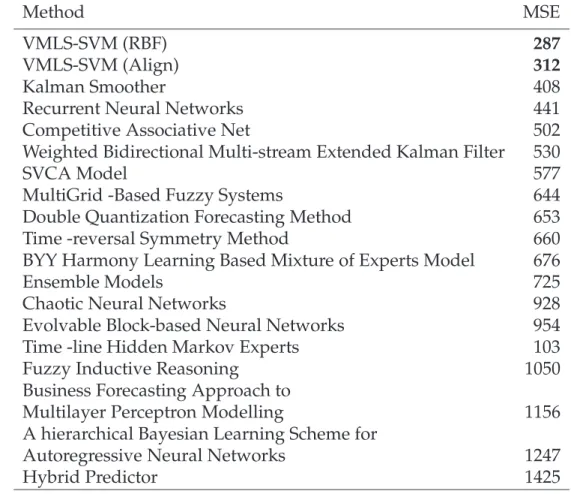
Table3.2shows a comparison between our method (labeled as VMLS-SVM) and the best results reported for this series in the competition. Table 3.2
con-Table 3.2: Comparison between the main methods on CATS benchmark.
Method MSE
VMLS-SVM (RBF) 287
VMLS-SVM (Align) 312
Kalman Smoother 408
Recurrent Neural Networks 441
Competitive Associative Net 502
Weighted Bidirectional Multi-stream Extended Kalman Filter 530
SVCA Model 577
MultiGrid -Based Fuzzy Systems 644
Double Quantization Forecasting Method 653
Time -reversal Symmetry Method 660
BYY Harmony Learning Based Mixture of Experts Model 676
Ensemble Models 725
Chaotic Neural Networks 928
Evolvable Block-based Neural Networks 954 Time -line Hidden Markov Experts 103
Fuzzy Inductive Reasoning 1050
Business Forecasting Approach to
Multilayer Perceptron Modelling 1156
A hierarchical Bayesian Learning Scheme for
Autoregressive Neural Networks 1247
Hybrid Predictor 1425
tains just the best results of our models, using D = 1, 000, C = 0.01 and WS =80 parameter values.
3.3.3 Results on the Dataset of NN3 Neural Forecasting
Competition
To further investigate the capabilities of VMLS-SVM, we made a comparison with ǫ-insensitive SVM regression method. Hence we applied our method to
forecast the reduced subset of time series of the NN3 Artificial Neural Network and Computational Intelligence Forecasting Competition, which has reported results using anǫ-insensitive SVM regression approach [32].
3.3. EXPERIMENTAL RESULTS
30
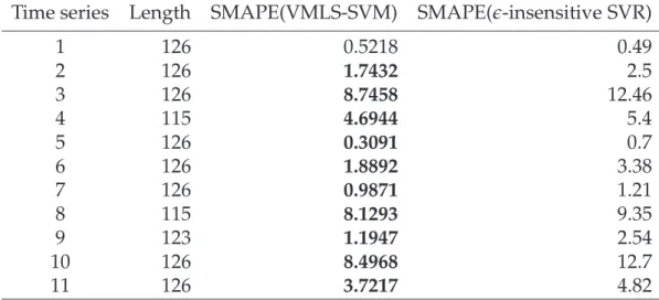
Table 3.3: SMAPE of each time series using the VMLS-SVM andǫ-insensitive
SVM regression methods.
Time series Length SMAPE(VMLS-SVM) SMAPE(ǫ-insensitive SVR)
1 126 0.5218 0.49 2 126 1.7432 2.5 3 126 8.7458 12.46 4 115 4.6944 5.4 5 126 0.3091 0.7 6 126 1.8892 3.38 7 126 0.9871 1.21 8 115 8.1293 9.35 9 123 1.1947 2.54 10 126 8.4968 12.7 11 126 3.7217 4.82
series is 1241, and there is no domain knowledge about the time series. In [32],
each the last 18 values of each time series were predicted. The evaluation met-ric was the symmetmet-ric mean absolute percent error (SMAPE) [8,60]:
SMAPE= 1 n n
∑
i=1 |yi−yˆi| (yi+yˆi)/2 ·100, (3.18) where n is the number of prediction, ˆyi is the ith prediction and yi is the ith expected value from the evaluation set.For each time series, we defined 18 different prediction functions based on Eq. 3.15. Each prediction function used the same parameter setting, but each times series used different parameter setting, which were determined by parameter optimization. To carry out the parameter optimization, we made three subsets from each time series e.g. the training set, the validation set and the evaluation set. Each evaluation set contains the last 18 values from the corresponding time series, and each validation set is made up from the last 18 values of the corresponding time series without the evaluation set. For each set triplet, we made a hyper-parameter optimization for the VMLS-SVM based prediction functions, using the training and validation sets. We adjusted only
the D and C parameters during the optimization and used a fixed window size WS=12, and RBF kernel with parameterγ=0.001. These optimizations determined well-generalization parameter sets for each VMLS-SVM predictor. Afterwards, we used the correct parameter setups; we trained each VMLS-SVM prediction function on the training and validation sets and evaluated them on the evaluation set as test set. Table3.3shows a comparison between our method and the results reported for this series in [32].
The mean SMAPE of our method is 3.6757 and the same value of the ǫ
-insensitive SVM regression method is 5.05. Hence we can assess that our method using VMLS-SVM methods and parameter optimization achieves a significantly higher mean performance. As can be seen, our method achieves lower SMAPE on each time series except the first one.
3.3.4 Results on the Santa Fe Data Set D
Here we present the results of our method on a widely-recognized benchmark, the D data series from the Santa Fe competition [121]. The data set consists of artificial data generated from a nine-dimensional periodically driven dissipa-tive dynamical system with an asymmetrical four-well potential and a drift on the parameters.
This database has a relatively high dimension, it is large (100,000 data points) and highly dynamic. Moreover, we have no background information about it.
Our evaluation is measured by the Root Mean Squared Error (RMSE) met-ric: RMSE= s 1 n n
∑
i=1 (yi−yˆi)2, (3.19)where the notation is similar to the one was used in Eq.3.17, and we predict 25 missing values.
This data set is quite large, which implies that it is a computationally inten-sive learning task. Hence we trained our system with only one configuration: We used only the last 20,000 training samples applying the RBF kernel with
γ=0.001. The window size was 80, the value of parameter D was 1,000, and the value of parameterC was 0.01. These parameters were determined using
3.4. CONCLUSIONS
32
Table 3.4: Comparison between the methods on Santa Fe D data set.
Method RMSE VMLS-SVM (RBF) 0.0628 SVM (ǫ-insensitive) 0.0639 SVM (Huber) 0.0653 RBF network 0.0677 ZH [126] 0.0665 our experiments with the earlier tested benchmarks.
Table3.4shows the results of our method relative to the methods proposed by Müller et al. [87]. The presented results show that our methods can achieve a better performance than others in this task as well.
3.4 Conclusions
In this chapter we presented a novel extension for LS-SVM based on weighting the variance of error. After presenting the basic theory of the method, we eval-uated it on publicly available benchmarks. These experiments show that the proposed method can indeed achieve a higher efficiency on the three differ-ent, widely-recognized benchmarks than the standard LS-SVM or other sim-ilar methods. The nice results we obtained can probably be attributed to the beneficial features of our novel method, since the data sets we used for exper-iments are typical and widely-used benchmarks for testing machine learning algorithms for time series prediction.
Moreover, we showed that with a carefully designed extension a basic SVM approach (LS-SVM) can be successfully adapted to a specific task (time se-ries forecasting) resulting a much suitable approach. Additionally, one can see that formalizing a preliminary observation into the SVM-based framework is straightforward. We believe that the proposed method—and additionally how we obtained—confirms the robustness of the SVM-based learning.
Transformation-based Domain Adaptation
The generalization properties of most statistical machine learning approaches are based on the assumption that the samples of the training dataset come from the same underlying probability distribution than those that are used in the prediction phase of the model. Unfortunately—mainly in real-world applications—this assumption often fails. There are numerous Natural Lan-guage Processing (NLP) tasks where plentiful labeled training databases are available from a certain domain (source domain), but we have to solve the same task using data taken from a different domain (target domain) where we have only a small dataset. Manually labeling the data in the target domain is costly and inefficient. However, if an accurate statistical model from the source domain is presented, we can adapt it to the target domain [36]. This process is calleddomain adaptation.
Opinion mining aims at automatically extracting emotional cues from texts [72]. For instance, it can classify product reviews according to the customers positive or negative polarity. This is a typical problem where the requirement for domain adaptation is straightforward as there exists numerous slightly dif-ferent domains (e.g. difdif-ferent products are difdif-ferent domains), and the
con-4.1. RELATED WORK
34
struction of manually labeled training data for each of them would be costly.Here, we will define a general framework to directly capture the relations between domains. In order to experimentally evaluate our approach, SVM and Logistic Regression [15] were plugged into the framework and the approach was compared to a number of baseline algorithms and published results on opinion mining datasets. We will show that SVM is a more suitable approach to apply in the proposed framework.
The results presented here are mainly based on our earlier work [91].
4.1 Related Work
Numerous preliminary algorithms have been developed in the field of domain adaptation, which roughly can be categorized into two mainstreams.
One of these types of methods tries tomodel the differences between the distri-butionsof the source and target domains empirically. In [28] the parameters of a maximum entropy model are learnt from the source domain, while an adapted Gaussian prior was used during training a new model on target data. A dif-ferent technique proposed in [36] defines a general domain distribution that is shared between source and target domains. In this way, each source (target) example can be considered a mixture of source (target) and general distribu-tions. Using these assumptions, their method was based on a maximum en-tropy model and used the EM algorithm for training. Another approach was proposed in [35], where a heuristic nonlinear mapping function was used to map the data into a higher dimensional feature space where a standard super-vised learner could be applied in order to perform the domain adaptation.
Another generation of domain adaptation algorithms are based on defin-ing new features for capturdefin-ing the correspondence between source and target do-mains [12, 47]. In this way, the two domains appear to have very similar dis-tributions, which enables effective domain adaptation. In [17], the authors proposed a method—called Structural Correspondence Learning (SCL) algo-rithm—which depends on the selection of pivot features that appear frequently in both the source and the target domains. Although it was experimentally shown that SCL can reduce the difference between domains ba