A geostatistical model for combined analysis of
point-level and area-level data using INLA and SPDE
Paula Moragaa,∗, Susanna M. Cramba,b, Kerrie L. Mengersena,c, Marcello Paganod
aARC Centre of Excellence for Mathematical & Statistical Frontiers, Queensland University
of Technology (QUT), Brisbane, Australia
bCancer Council Queensland, Brisbane, Australia cCooperative Research Centre for Spatial Information, Australia
dDepartment of Biostatistics, Harvard T.H. Chan School of Public Health, Boston, United
States
Abstract
In this paper a Bayesian geostatistical model is presented for fusion of data obtained at point and areal resolutions. The model is fitted using the INLA and SPDE approaches. In the SPDE approach, a continuously indexed Gaussian random field is represented as a discretely indexed Gaussian Markov random field (GMRF) by means of a finite basis function defined on a triangulation of the region of study. In order to allow the combination of point and areal data, a new projection matrix for mapping the GMRF from the observation locations to the triangulation nodes is proposed which takes into account the types of data to be combined. The performance of the model is examined and compared with the performance of the method RAMPS via simulation when it is fitted to i) point, ii) areal, and iii) point and areal data to predict several simulated surfaces that can appear in real settings. The model is applied to predict the concentration of fine particulate matter (PM2.5), in Los Angeles and Ventura
counties, United States, during 2011.
Keywords: Misalignment, Data fusion, Model-based geostatistics, INLA, SPDE
∗Paula Moraga, School of Mathematical Sciences, Queensland University of Technology,
1. Introduction
Spatial and spatio-temporal data arise in a wide range of scientific disciplines, including the environmental, epidemiological, geographical and ecological fields [1]. Data are typically observed either at points in space (point data), or over areal units such as counties or postal codes (areal data). Examples include air 5
pollution measurements taken at a set of ambient stations, temperature and precipitation measurements from weather stations, and population sizes from census tracts. In epidemiology, point data arise when the locations at which cases of disease occur are available, and areal data are often reported when point data are aggregated over geographical subregions of the region of study 10
due to ethical concerns over data use and patient confidentiality [2].
Spatially misaligned data are becoming increasingly common due to ad-vances in both data collection and management, as well as to the ability to merge data from large databases such as disease registries. When information is available from multiple sources on different scales, data may be fused to exam-15
ine just one variable, such as disease counts recorded in different administrative units. Here the aim is interpolation [3]. Alternatively, we might wish to relate one variable to other variables that are available at different spatial resolutions and alignments. An example is determining whether the risk of an adverse out-come provided at zip level is related to exposure to an environmental pollutant 20
measured at a network of stations, after adjusting for population at risk and other county level demographic information. Here the aim is regression [3].
In this paper we will focus on the data fusion problem which seeks to learn about a particular variable by combining data that are available at different spatial scales. Others have previously developed Bayesian models enabling fu-25
sion of data obtained at areal and point-referenced resolutions via the use of latent point-level processes [4] , hierarchical downscaling [5], modelling data conditional on the resolution [6], and the use of algorithms such as the repa-rameterized and marginalized posterior sampling (RAMPS) [7].
Markov chain Monte Carlo (MCMC) based methods. These methods have made a great impact on statistical practice by making Bayesian inference tractable for complex models but they also present a wide range of problems in terms of con-vergence and computational time [8]. In this paper we propose general and flexible hierarchical Bayesian models to analyze spatially misaligned data. In 35
order to fit the models, we resort to the Integrated Nested Laplace approx-imation (INLA) [9] and the Stochastic Partial Differential Equation (SPDE) [10] approaches which are a computationally effective alternative to MCMC for Bayesian inference. In order to allow the combination of data at different spa-tial resolutions, we propose a new projection matrix for mapping the GMRF in 40
the SPDE method which takes into account how the different types of data are collected. This new approach is fast and flexible.
The outline of the paper is as follows. First, we present flexible models for handling spatial misaligned data in fusion problems. Then, we briefly introduce the INLA and SPDE approaches for Bayesian inference, and present the pro-45
jection matrix that allows the combination of point and areal data. In Section 3, a simulation study is carried out to compare the performance of the model when estimating several simulated surfaces using point, areal, and point and areal data combined. Then, in Section 4 we evaluate the model in comparison to the RAMPS alternative method for data fusion by applying the methods to 50
several simulated data scenarios. In Section 5, we present an application of the model to real data showing spatial misalignment. In this application, we ob-tain the spatial distribution of fine particulate matter (PM2.5), in Los Angeles
and Ventura counties, United States, during 2011. Finally, the conclusions are presented.
55
2. Models and Inference
2.1. Models
process. This process is denoted by S = {S(x) : x ∈ D ⊂ R2}, has mean function E[S(x)] = 0 and stationary covariance function Cov(S(x), S(x0)) = Σ(x−x0). Conditionally on S, point data Yi observed at a finite set of sites, sayxi∈D,i= 1,2, . . . , I, are mutually independent with
Yi|S(xi)∼N(µ(xi) +S(xi), τ2),
whereµ(xi) represents the large scale structure. Areal data observations arise
as block averages in blocksBj⊂D,j= 1,2, . . . , J,
Y(Bj) =|Bj|−1
Z
Bj
(µ(x) +S(x))dx, |Bj|>0,
where|Bj|=
R
Bj1dxdenotes the area ofBj.
These models can also accommodate explanatory covariates by including them in the large scale part of the model. Moreover, the models can also be ex-60
tended to include random effects that can deal with other sources of variability.
2.2. Inference
We fit the models by using the INLA [11, 9] and SPDE approaches [10] which can be easily applied using theR packageR-INLA [12]. INLA uses a combina-tion of analytical approximacombina-tion and numerical integracombina-tion to do approximate 65
Bayesian inference in latent Gaussian models which includes a large class of models ranging from generalized linear mixed to spatial and spatio-temporal models.
The combination of INLA and SPDE permits analysis of point-level data. In the SPDE approach, the continuously indexed Gaussian fieldSis represented as a discretely indexed Gaussian Markov random field (GMRF) by means of a finite basis function defined on a triangulation of the region of study. Specifically,
S(x) =
G
X
g=1
ψg(x)Sg,
where,ψg(·) denotes piecewise polynomial basis functions on each triangle,{Sg} are zero-mean Gaussian distributed weights, andG are the number of vertices 70
In the SPDE approach, the covariance function of the Gaussian field S is required to belong to the Mat´ern family which represents a very flexible class of covariance functions that appears naturally in many scientific fields [13]. Specifically, for locations xi and xj ∈ R2, the Mat´ern covariance function is defined as
Cov(S(xi), S(xj)) = σ2
2ν−1Γ(ν)(κ||xi−xj||)
νKν(κ||x
i−xj||).
Here, Kν is the modified Bessel function of second kind and order ν >0. The integer value of ν determines the mean square differentiability of the process and it is usually fixed since it is poorly identified in applications. σ2 denotes
the variance and κ > 0 is related to the range ρ, the distance at which the 75
spatial correlation is close to 0.1 [14].
2.3. Approximation of integrals
In practice, the integrals appearing in the models proposed may not be available in a closed-form. In our approach, we will approximate them using the representation of the continuous Gaussian random field as a GMRF provided by the SPDE approach. Thus,
Z
Bj
S(x)dx≈
G
X
g=1 AjgSg,
where G is the number of vertices in the triangulation, {Sg} are zero-mean Gaussian distributed weights, andA is a J ×G sparse matrix that maps the GMRF from theJ observation locations to theGtriangulation nodes.
80
The matrixAspecified in the SPDE approach is designed to deal with point-referenced data. To adapt this approach to our problem, we need to make some modifications that allow accommodation of both point and areal data. Specifically, for the construction of A, we need to differentiate between point and areal observations. If we consider observations taken at point locations in 85
the study region, the projection matrixAcan be chosen in the same way as in the SPDE approach. Thus, the rowiinAcorresponding to an observation at point
vertices of the triangle that contains the point. Ifxiis within the triangle, these
values are equal to the barycentric coordinates. That is, they are proportional 90
to the areas of each of the three subtriangles defined by the point xi and the
triangle’s vertices, and sum to 1. Ifxi is equal to a vertex of the triangle, row iwill have just one non-zero value equal to 1 at that vertex. Intuitively, if we assume that each triangulation vertex has a weight given by the GMRFS, the value ofS(x) at a location that lies within one triangle, is the projection of the 95
plane formed by the triangle vertices weights at locationx.
On the other hand, the model specifies that a particular observation in an area B and the process S are linked through the mean value of the random field in the entire area: |B|−1R
BS(x)dx, where|B|denotes the area of B. As
a result, the rows ofAcorresponding to a particular observation in an area will 100
have non-zero values in all vertices inside the area and will be equal to 1/H, whereHis the number of vertices within the area. Here we need to note that we approximate the integral of the process in the area by an average of all vertices weights inside the area. Therefore, to minimize the error of the approximation, it is important to construct a fine triangulation of the domain.
105
TheRcode for the combined analysis of point-level and area-level data using this approach is provided in the Appendix.
3. Simulation study
In this section we carry out a small simulation study to assess the perfor-mance of the method when predicting different spatial surfaces combining data 110
that have been obtained at several configurations of points and areas in the region of study. First, we generate several spatial surfaces that may reproduce some of the situations that can appear in real settings. Then, for each of the surfaces, the model is fitted using point and areal measurements of the surfaces taken at different configurations. Finally, the merits of the model in each of 115
simulations, the models used to generate the spatial surfaces, the models fitted, and the results of the simulation study.
3.1. Simulated data 120
We are interested in testing the method in a range of situations that can appear in real settings. To do so, we decide to simulate several spatial surfaces of phenomena that can have continuous values inR. These data may represent, for example, concentration levels of some air pollutant, and may be measured directly at points where monitoring stations are located, or may be obtained 125
at cells of a regular grid produced by numerical models. In our simulation, we consider the unit square as the study region and take observations at different configurations of randomly generated points and regular grids and vertical bands over the region of study.
The different data scenarios are created by varying the number of points 130
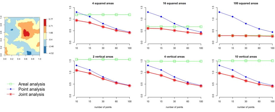
and areas in the data sets to be combined. Specifically, data sets of 10, 15, 30, 60 and 100 points are combined with data sets of 4, 16 and 100 squared areas, or 2, 4 and 10 vertical areas. We also create scenarios with no point data and scenarios with no areal data. Examples of such configurations are shown in Figure 1.
135
We construct four surfaces for simulated data. For locationsxi in the unit
square, observationsYi inRare simulated as follows:
Yi=ziβ+S(xi), i= 1, . . . , n,
where zi = (1, zi) denotes the vector of the intercept and covariates, β =
(β0, βc)0 is the coefficient vector, and S is a zero-mean Gaussian field with
Mat´ern covariance function with varianceσ2 and range ρ. In the simulations, we set the interceptβ0= 0,σ2equal to 4 or 1 andρequal to 0.7 or 0.1. Moreover,
we use as a covariate a geographic trend withβc = 2. The trend covariate is 140
calculated as (x2
i−x2), wherex2i is the second coordinate of locationxi, andx2
Figure 1: Examples of point and areal configurations used in the simulation study.
represent a surface that reflects changes in temperature or other environmental covariates that are related with latitude. The values of the parameters for each 145
of the simulated surfaces are presented in Table 1. Examples of the simulated surfaces are shown in Figures 2 to 5.
covariate βc σ2 ρ
US1 - - 4 0.7
US2 - - 1 0.1
US3 trend 2 4 0.7 US4 trend 2 1 0.1
Table 1: Parameters of the models used to generate the surfaces in the simulation study.
3.2. Fitted models
Let Yi, i = 1, . . . , n+m, denote the simulated observations at points xi, i= 1, . . . , n, and areas Bi, i=n+ 1, . . . , n+m. The fitted models assume a
[image:8.612.232.379.456.544.2]forµiin the second level:
µi=ziβ+S(xi), i= 1, . . . , n,
µi=ziβ+|Bi|−1
Z
Bi
S(x)dx, i=n+ 1, . . . , n+m.
Here, zi = (1, zi) denotes the vector of the intercept and the covariate, β= (β0, βc)0 is the coefficient vector, andS is a zero-mean Gaussian field with
150
Mat´ern covariance function with parametersσ2andρ. If the data are simulated
without a covariate, the fitted models do not incorporate the covariate term. If they are simulated using a covariate, the models incorporate the effect of the same covariate.
The models are fitted assuming the following prior distributions. The model 155
parameter ν is set fixed to 1 in the Mat´ern function implying a continuous domain Markov field. We assign a flat improper prior to the interceptβ0, and
a zero-mean Gaussian distribution with precision equal to 0.001 for the effect of the covariate. Finally, S ∼N(0, Q−1) whereQis a sparse precision matrix
depending on hyperparametersκandσ2.
160
3.3. Results
For each simulated pattern, we generate point and areal data and predict the simulated surface applying the model to i) point, ii) areal, and iii) point and areal data combined. We generate 100 surfaces from each simulated scenario to have stable results. The merits of the model in each situation are assessed using the mean squared errors (MSE) of the predictions. The MSE for each simulated data set is calculated as
MSE = 1
R
X
x∈R
(u(x)−uˆ(x))2
!1/2
,
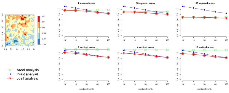
whereRdenotes the number of locations in the study region,u(x) is the value of the simulated surface at locationx, and ˆu(x) is the prediction ofu(x). Figures 2 to 5 show the MSEs for each of the scenarios and combinations of data averaged over the 100 replications.
The results show that the MSE depends on the simulated surfaces and also on the types of data used to fit the model. We observe that when the model is applied using data obtained in just areas or points, the MSE decreases as the number of areas or points increases. There are some situations, however, where the decrease of MSE is very small. This is the case of scenario US2 170
where the data are generated usingσ2= 1,ρ= 0.1 and with no covariates. We
also see that in general, the combination of point and areal data provides better predictions than if the method is applied just to one type of data. There are a few exceptions however. For example, when there is a large amount of areal or point data then information from just one type of data could be enough to accurately 175
predict the real process. In these situations, a joint analysis is not useful to improve the predictions obtained using a point or areal analysis. For example, if there are 100 squared areal observations and just a few point observations, the addition of point data to the analysis does not provide additional information to obtain better predictions.
[image:10.612.94.552.393.582.2]180
Figure 3: Scenario US2 results. First column: one of the 100 simulated surfaces. Second to fourth columns: MSEs of the predictions obtained for the simulated surfaces US2 averaged over 100 replications by type of analysis.
4. Performance evaluation in comparison with RAMPS
In this section, we compare the method presented with another existing method for data fusion. Specifically, we present a performance evaluation of our method in comparison with the reparameterized and marginalized posterior sampling (RAMPS) algorithm for complex Bayesian geostatistical models. We chose RAMPS for comparison because of its flexibility and the availability of anRpackage calledrampsthat implements all of its capabilities [15]. RAMPS enables joint modeling of areal and point data arising from the same underly-ing spatial process, and allows accommodation of non-spatial correlation and variance heterogeneity as well as spatial and/or temporal correlation. Specifi-cally, an observation vectorY which may contain both point and areal data is modeled as follows:
Y =Xβ+W γ+KZ+,
Figure 4: Scenario US3 results. First column: one of the 100 simulated surfaces. Second to fourth columns: MSEs of the predictions obtained for the simulated surfaces US3 averaged over 100 replications by type of analysis.
whereβ is a vector of regression coefficients,γis a vector of non-spatial random effects, Z is an vector of spatial random effects, is a vector of measurements errors, and the matrices X, W, and K are design matrices for fixed effects, non-spatial random effects, and spatial random effects, respectively. The model 185
is fitted using an algorithm that involves reparameterizing the variance param-eters, reformulating the means structure, marginalizing the joint posterior dis-tribution, and applying the slice sampling MCMC method based on simplexes. Here, we simulate four surfaces with different characteristics and obtain point and areal observations. Then, our method and RAMPS are applied to predict 190
the simulated surfaces using all the observations combined. Finally, the per-formance of the methods is evaluated by means of the MSE, the parameter estimates and the run time.
The four spatial surfaces are generated on [0,1]×[0,1] using a Gaussian model with a Mat´ern covariance structure with varianceσ2, rangeρand overall 195
meanβ0 = 0. For surfaces S1 and S3, we setσ2 = 4 and ρ= 0.7, in surfaces
Figure 5: Scenario US4 results. First column: one of the 100 simulated surfaces. Second to fourth columns: MSEs of the predictions obtained for the simulated surfaces US4 averaged over 100 replications by type of analysis.
geographic trend covariate calculated as (x2
i −x2) and coefficient βc = 2. The
observations to be combined are obtained as the point values corresponding to 100 randomly generated locations and the average values in the cells of a 4×4 200
regular grid. The surfaces generated and the areal and point observations for each scenario are shown in Figure 6.
We apply our method and RAMPS to predict the simulated surfaces. Let
Yi, i= 1, . . . , n+m, denote the simulated observations at pointsxi,i= 1, . . . , n,
and areasBi,i=n+1, . . . , n+m. The model fitted assumes a Normal likelihood
with meanµi expressed as
µi=ziβ+S(xi), i= 1, . . . , n,
µi=ziβ+|Bi|−1
Z
Bi
S(x)dx, i=n+ 1, . . . , n+m.
Here,zi = (1, zi) is the vector of the intercept and the covariate,β= (β0, βc)0
is the coefficient vector, andS is a zero-mean Gaussian field with Mat´ern co-variance function with parametersσ2 and ρ. This model is fitted to the data 205
fitted model does not incorporate the covariate term. Due to the large amount of time needed to fit the model using RAMPS, prediction is just done at 231 uniformly distributed locations.
The priors used when applying our method are the same as the ones em-210
ployed in the simulation study in Section 3. When applying RAMPS, flat priors are used on the interceptβ0 and the covariate coefficientβc. An inverse gamma
prior with shape and scale parameters set to 0.01 is used forσ2, and an uniform
prior on (0, 2) is used for the rangeρ. Using RAMPS, convergence is achieved running a MCMC chain of 30,000 iterations and using a burn-in of 1,000 and 215
a thinning rate of 30 iterations for each of the surfaces. Posterior means and 95% CIs are calculated with the remaining 966 iterations. We note that the use of different priors may result in different estimates and run times. How-ever, showing results from even only these priors reveals the main differences in performance between our method and RAMPS.
220
For each of the simulated surfaces and methods, we calculate the MSE, the posterior means and 95% CIs for the model parameters, and the run times. These values are shown in Table 2. We observe that lower MSEs are obtained with our method than with RAMPS in all surfaces except for surface S2, where ours is 0.02 higher (0.89 with our method and 0.87 with RAMPS). The highest 225
difference in MSE is obtained when the methods are applied to predict surface S3 which is simulated using a geographic trend as a covariate, σ2 = 4 and
ρ= 0.7. In S3, the MSE obtained with our method is equal to 0.46 compared to 1.75 with RAMPS. We see that neither our method nor RAMPS accurately recover the true values of the parameters used in the simulations, both methods 230
yield 95% CIs that contain the true values for most of the parameters. We also see that in the simulated surfaces S1 and S3, that is, whenσ2= 4 andρ= 0.7,
the upper limits of the 95% CIs forσ2 obtained with RAMPS are very high.
With our method, however, narrower 95% CIs forσ2 are obtained. Finally, we
note that RAMPS needs longer run times than our method. Specifically, for all 235
5. Application to air pollution data
The methodology proposed provides a valuable tool in a wide range of re-search fields. Here, we present an application where we obtain the spatial dis-240
tribution of a common air pollutant: fine particulate matter (PM2.5) in Los
Angeles and Ventura counties, United States, during 2011. We fit a spatial model combining information for the variable of interest from point and areal resolutions. We also model point and areal data separately to assess the differ-ences in the predictions obtained.
245
Particulate matter, or PM, are a mixture of microscopic solids and liquid droplets floating in the air that are considered harmful to public health and the environment [16]. These particles are made up of a number of components such as acids, chemicals, metals, soil and dust, and are emitted in the atmosphere either directly from a source or as result of complicated chemicals reactions. 250
Particulate matter which are less than 2.5µm in diameter (PM2.5) pose one of
the greatest problems since they can get deep into the lungs and cause serious health effects including increased respiratory symptoms, heart or lung diseases, and even premature death [16].
Information on concentration (micrograms per cubic meter) for PM2.5 in
255
Los Angeles and Ventura counties are available as direct measurements at loca-tions of monitoring sites, and as estimates inferred from satellite-derived PM2.5
sources at a raster grid. The monitoring data have been obtained from a set of 14 sites sparsely located in the region at which the United States Environ-mental Protection Agency (EPA) regularly measures PM2.5 among other air
260
pollutants [17] We have used the mean of the daily measurements recorded in year 2011 in each of the monitoring stations. The satellite-derived estimates rep-resent three-year mean grids (2010-2012) of PM2.5concentrations derived from
a combination of MODIS (Moderate Resolution Imaging Spectroradiometer), MISR (Multi-angle Imaging SpectroRadiometer) and SeaWIFS (Sea-Viewing 265
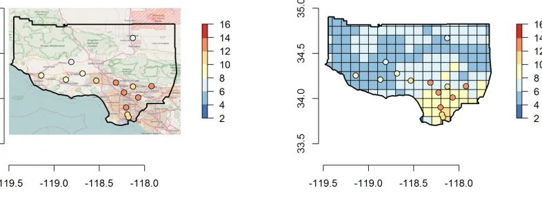
or approximately 10 km at the equator). Figure 7 shows the concentration values in each of the monitoring stations and in the raster grid.
The model used to predict PM2.5 values in the study region is specified as
follows. The PM2.5concentration,Yi, at each of the locations of the monitoring
stations,xi,i= 1, . . . , n, and cells of the raster grid,Bi, i=n+ 1, . . . , n+m,
are modeled as Gaussian observations with meanµi:
Yi∼Normal(µi, σ2), i= 1, . . . , n, n+ 1, . . . , n+m,
µi=β0+S(xi), i= 1, . . . , n,
µi=β0+|Bi|−1
Z
Bi
S(x)dx, i=n+ 1, . . . , n+m,
where β0 is the intercept and S is a zero-mean Gaussian field with Mat´ern
270
covariance function with parameters σ2 and ρ. We fit the model three times
using areal, point and areal and point data. The model is fitted using the same priors as the ones employed in the simulation study in Section 3.
Although estimates differed by analysis the 95% CIs overlapped (Table 3). The most accurate predictions (tightest CIs) for model parameters were gener-275
ally for the areal model, then our model, while using only the point data resulted in large uncertainty around the estimates.
Maps of the predictions obtained and the 95% CI showing the range of plausible values for each location are shown in Figure 8. Although all maps show a predicted PM2.5higher in the south, there are some differences depending on
280
the analysis used. For example, with the joint analysis the predicted PM2.5 is
higher close to the city of Los Angeles than the predicted PM2.5 obtained with
the areal analysis. Also, by using both areal and point data, we are able to obtain more accurate predictions in the south where there is both point and areal information than the ones obtained using just one type of data.
285
6. Discussion
spatially continuous variable that can be modeled using a Gaussian random field process. INLA and SPDE approaches were used to fit the data and represent 290
the continuously indexed Gaussian random field as a discretely indexed GMRF by means of a basis function representation defined on a triangulation of the region of interest. In order to allow the combination of point and areal data, we proposed a new projection matrix for mapping the GMRF from the observation locations to the triangulation nodes which takes into account the types of data. 295
The results show that the goodness of fit depends on the simulated surfaces and also the types of data used to fit the model. In most situations we observe that the combination of point and areal data provides better predictions than if the method is applied to just one type of data, and this was consistent over both simulated and real data. Our method was also demonstrably superior to 300
RAMPS by obtaining better predictions in much shorter run times on simulated data.
Real data are messy, especially when attempting to use multiple sources of information. Our method performed well when applied to monitored air pollution data. When predicting the concentration of PM2.5 in Los Angeles
305
and Ventura counties during 2011, the point analysis gave markedly different results to the areal analysis (Figure 8). In part, this may be due to differences in time periods, as well as the relative lack of monitoring stations in the north. Combining these estimates using our method enabled more accurate predictions of the concentration of PM2.5, particularly in the south.
310
A limitation of the method proposed is that it is only applicable to Gaussian data. Unfortunately, this does not include many important settings such as disease mapping problems where data are typically modelled using Poisson or Binomial distributions and non-identity link functions.
Models based on aggregated data contain the potential for ecological fallacy 315
to the grouping of individuals, and the specification bias due to the differential 320
distribution of confounding variables created by grouping [20], [21]. In many situations, however, it is difficult to obtain sufficient point data to obtain con-clusions and we should make the most of the information from the available data regardless of their spatial resolution. For example, [22] show how the com-bination of disease data from different sources can improve inferences from that 325
using a single data set, and demonstrate that analyses combining related data at both the individual and aggregate level can reduce ecological bias and add precision.
There are many situations where data are very hard to obtain and especially in these cases it is very important to optimize the use of all available informa-330
tion. The method proposed enables obtaining better predictions by combining data obtained at different resolutions. However, we should be aware that bias could arise if we combine data that are not completely comparable such as data collected about different populations or at different times. In such situations we may decide to use just one of the data sets or alternatively to adjust for bias in 335
the model.
A major advantage of the method presented is that the Bayesian framework used could be easily extended to adequately model many problems of interest. For example, the model may be extended to accommodate spatio-temporal data as follows. Let us consider a spatio-temporal Gaussian process S ={S(x, t) :
x ∈ D ⊂ R2, t ∈ T ⊂ R} with E[S(x, t)] = 0 and stationary covariance function Cov(S(x, t), S(x0, t0)) = Σ(x−x0, t−t0). Data observed at locations
xi, i= 1, . . . , I, and timestk, k= 1, . . . , K may be modeled as
Yi,k|S(xi, tk)∼N(µ(xi, tk) +S(xi, tk), τ2).
Then, observations in areasBj⊂D,j= 1,2, . . . , J, and periods of timeτl∈T, l= 1, . . . , L, are expressed averaging the process in space and also in time,
Y(Bj, τl) =|Bj|−1|τl|−1
Z
Bj
Z
τl
(µ(x, t) +S(x, t))dxdt, |Bj|>0, |τl|>0.
sources of uncertainty, including sampling error, measurement error, as well as prediction errors at unsampled locations. Another advantage of the method is that by using the approximate methods INLA and SPDE, we are able to obtain 340
results quickly and avoid assessing the convergence and mixing properties of the chains generated by using MCMC-based methods. In addition, since this method is less computationally intensive we are able to deal with large data sets.
The combination of point-level and area-level referenced data is an important 345
and not yet completely resolved methodological issue within the general area of spatial statistics. We think that the approach presented may be a helpful advance in this area by providing a useful tool that is applicable in a wide range of situations where information at different spatial resolutions is combined.
Acknowledgements
350
PM would like to acknowledge the financial support for this research from NIH/NIAID grant R01AI097015-01A1 and ARC Australian Laureate Fellowship FL150100150.
References
[1] N. Cressie, Statistics for spatial data, Wiley, New York, 1993. 355
[2] A. B. Lawson, Bayesian point event modeling in spatial and environmental epidemiology, Statistical Methods in Medical Research 21 (2012) 509–529.
[3] S. Banerjee, B. P. Carlin, A. E. Gelfand, Hierarchical modeling and analysis for spatial data, Second Edition, Chapman and Hall/CRC, Boca Raton, 2014.
360
[5] V. J. Berrocal, A. E. Gelfand, D. M. Holland, A spatio-temporal downscaler for outputs from numerical models, J. Agric. Biol. Environ. Stat. 15 (2010) 365
176–197.
[6] C. K. Wikle, L. M. Berliner, Combining information across spatial scales, Technometrics 47 (1) (2005) 80–91.
[7] M. K. Cowles, J. Yan, B. Smith, Reparameterized and marginalized pos-terior and predictive sampling for complex bayesian geostatistical models, 370
Tech. rep., The University of Iowa, Department of Statistics and Actuarial Science (2007).
URLhttp://www.stat.uiowa.edu/techrep/
[8] B. M. Taylor, P. J. Diggle, INLA or MCMC? A tutorial and comparative evaluation for spatial prediction in log-Gaussian Cox processes, Journal of 375
Statistical Computation and Simulation 84 (10) (2014) 2266–2284.
[9] H. Rue, S. Martino, N. Chopin, Approximate Bayesian inference for la-tent Gaussian models by using integrated nested Laplace approximations, Journal of the Royal Statistical Society, Series B 71 (2) (2009) 319–392.
[10] F. Lindgren, H. Rue, J. Lindstr¨om, An explicit link between gaussian fields 380
and gaussian markov random fields: the stochastic partial differential equa-tion approach, Journal of the Royal Statistical Society, Series B 73 (4) (2011) 423–498.
[11] H. Rue, S. Martino, Approximate Bayesian inference for hierarchical Gaus-sian Markov random fields models, Journal of Statistical Planning and 385
Inference 137 (2007) 3177–3192.
[12] H. Rue, S. Martino, F. Lindgren, D. Simpson, A. Riebler, R-inla: Approx-imate bayesian inference using integrated nested laplace approximations,
http://www.r-inla.org/ (2013).
[13] P. Guttorp, T. Gneiting, Studies in the history of probability and statistics 390
[14] M. Cameletti, F. Lindgren, D. Simpson, H. Rue, Spatio-temporal model-ing of particulate matter concentration through the spde approach, AStA Advances in Statistical Analysis.
[15] B. J. Smith, J. Yan, M. K. Cowles, Unified geostatistical modeling for 395
data fusion and spatial heteroskedasticity with r package ramps, Journal of Statistical Software 25 (10) (2008) 1–21.
[16] United States Environmental Protection Agency (EPA), Particulate Matter (PM) Pollution, https://epa.gov/pm-pollution(2015).
[17] United States Environmental Protection Agency (EPA), Air Qual-400
ity Data Mart, https://aqs.epa.gov/aqsweb/documents/data_mart_
welcome.html(2015).
[18] A. van Donkelaar, R. V. Martin, M. Brauer, B. L. Boys, Global annual pm2.5 grids from modis, misr and seawifs aerosol optical depth (aod), 1998-2012. palisades, ny: Nasa socioeconomic data and applications center 405
(sedac),http://dx.doi.org/10.7927/H4028PFS(2015).
[19] A. van Donkelaar, R. V. Martin, M. Brauer, B. L. Boys, Use of satellite observations for long-term exposure assessment of global concentrations of fine particulate matter, Environmental Health Perspectives 123 (2) (2015) 135–143.
410
[20] W. S. Robinson, Ecological correlations and the behavior of individuals, American Sociological Review 15 (1950) 351–357.
[21] C. A. Gotway, L. J. Young, Combining incompatible spatial data, Journal of the American Statistical Association 97 (459) (2002) 632–648.
[22] C. Jackson, N. Best, S. Richardson, Hierarchical related regression for com-415
Appendix
Rcode for combined analysis of point-level and area-level data using INLA 420
and SPDE.
# Point observations
# coop: matrix of point locations
# yp: vector of observed values at points
# xp: vector of covariate values at points
425
# Areal observations
# spol: SpatialPolygons object containing the areas
# cooa: matrix of the spatial coordinates of spol
# ya: vector of observed values in areas
430
# xa: vector of covariate values in areas
# Prediction points
# coopred: matrix with point locations for prediction
# ypred: vector of observed values in prediction points (NA)
435
# xpred: vector of covariate values in prediction points
# Mesh
# meshfit: fine triangulated mesh
440
# Matern SPDE model object
spde <- inla.spde2.matern(mesh=meshfit, alpha=2)
# Point observations
Ap <- inla.spde.make.A(mesh=meshfit, loc=coop)
445
stk.p <- inla.stack(tag=’point’,
data=list(y=yp),
effects=list(s=1:spde$n.spde, data.frame(b0=1, x=xp)))
450
# Areal observations
locin <- meshfit$loc[as.vector(which(!is.na(over(SpatialPoints(meshfit$loc), spol)))),]
block <- rep(0, nrow(locin))
for(i in 1:length(spol)){
block[as.vector(which(!is.na(over(SpatialPoints(locin), spol[i]))))] <- i
455
}
Aa <- inla.spde.make.A(mesh=meshfit, loc=locin, block=block, block.rescale="sum")
stk.a <- inla.stack(tag=’areal’,
data=list(y=ya),
A=list(Aa, 1),
460
effects=list(s=1:spde$n.spde, data.frame(b0=1, x=xa)))
# Prediction points
Apred <- inla.spde.make.A(mesh=meshfit, loc=coopred)
stk.pred <- inla.stack(tag=’pred’,
465
data=list(y=ypred),
A=list(Apred, 1),
effects=list(s=1:spde$n.spde, data.frame(b0=1, x=xpred)))
# Stack
470
stk.full <- inla.stack(stk.p, stk.a, stk.pred)
# Fit model
formula <- y ~ 0 + b0 + x + f(s, model=spde)
res <- inla(formula, data=inla.stack.data(stk.full),
475
Parameters values Simulated surfaces Areal observations Point observations
S1:
β0= 0 βc=− σ2= 4 ρ= 0.7
S2:
β0= 0 βc=−
σ2= 1 ρ= 0.1
S3:
β0= 0 βc= 2
σ2= 4 ρ= 0.7
S4:
β0= 0 βc= 2
[image:24.612.153.518.169.588.2]σ2= 1 ρ= 0.1
Figure 7: PM2.5concentration (micrograms per cubic meter) in monitoring stations (left) and
raster grid together with monitoring stations (right) in Los Angeles and Ventura counties in 2011.
β0 σ2 ρ
Joint analysis 7.31 (6.46 , 8.22) 2.72 (0.94 , 6.35) 1.20 (0.60 , 2.22) Areal analysis 7.50 (7.09 , 7.91) 3.74 (1.65 , 7.50) 0.85 (0.52 , 1.34) Point analysis 9.51 (5.42 , 12.94) 7.00 (1.78 , 20.2) 0.74 (0.31 , 1.55)
[image:26.612.145.464.532.602.2]Mean 2.5 percentile 97.5 percentile
Joint analysis
Areal analysis
[image:27.612.133.537.200.545.2]Point analysis
Figure 8: Posterior PM2.5 concentration (micrograms per cubic meter) by type of analysis,