Munich Personal RePEc Archive
Patterns of Competitive Interaction
Armstrong, Mark and Vickers, John
Department of Economics, Oxford University
July 2019
Online at
https://mpra.ub.uni-muenchen.de/95336/
Patterns of Competitive Interaction
Mark Armstrong
John Vickers
July 2019
Abstract
We explore patterns of competitive interaction by studying mixed-strategy equi-librium pricing in oligopoly settings where consumers vary in the set of suppliers they consider for their purchase. In the case of “nested reach” we …nd equilibria, unlike those in existing models, in which price competition is segmented: small …rms o¤er only low prices and large …rms only o¤er high prices. We characterize equilib-ria in the three-…rm case using correlation measures of competition between pairs of …rms. We then contrast them with equilibria in the parallel model with capacity con-straints. A theme of the analysis is how patterns of consumer consideration matter for competitive outcomes.
1
Introduction
In settings where consumers vary in the set of suppliers they consider for their purchase,
how do outcomes depend on the patterns of competitive interactions? The simplest
sit-uation in which this question arises is a duopoly in which each …rm has some captive
customers, while non-captive customers are able to choose whichever …rm’s o¤er they like
better. With more than two …rms, richer patterns of consideration become possible. Some
consumers may be captive to particular …rms, some might consider the o¤ers of all …rms, while others can choose among the o¤ers of various subsets of …rms. Competitive
out-comes, including patterns of price dispersion, then depend not only on the number and
…rms and their relative sizes, but also upon the pattern of consumer consideration of …rms.
The main aim of this paper is to explore this issue in an otherwise standard setting where
…rms compete in prices using mixed strategies.
There are various reasons why di¤erent consumers have di¤erent sets of choices open to them. Perhaps following a prior stage of advertising by …rms or search by consumers,
some might become aware of a di¤erent set of suppliers than do other consumers. For
instance, Honka et al. (2017, Table 1) document di¤erent levels of consumer awareness of
various retail banks in a local market. Alternatively, as in Spiegler (2006), there might
be horizontal product di¤erentiation such that each consumer considers only a subset of
products to be suitable. The set of …rms who are currently active in the market might be
uncertain (Janssen and Rasmusen (2002)) or the set of …rms who choose to post prices on a
comparison website might be uncertain (Baye and Morgan (2001)). Some consumers might
be constrained in their choices by location, transport costs or switching costs. For instance, some models of spatial competition, such as Smith (2004), suppose that a consumer
con-siders buying from those …rms located within a speci…ed radius of her. Consumers might
also di¤er in their ability to make comparisons between o¤ers, with confused consumers
choosing randomly between suppliers or buying from a default seller (Piccione and Spiegler
(2012), Chioveanu and Zhou (2013)). Our analysis does not take a view on the underlying
reason why consumers have di¤erent consideration sets. Rather, it takes the distribution
of consideration sets in the consumer population as given, and explores the consequences
for competition.
A considerable literature has explored aspects of this question, and some settings are
well understood—the case with symmetric sellers considered randomly, the case of
inde-pendent reach, and duopoly. (These special cases are discussed in more detail in section
2.) As to the …rst of these, Rosenthal (1980) and Varian (1980) considered the situation in
which some consumers are randomly captive to particular …rms, while others compare the
o¤erings of all …rms and buy from the cheapest. There is a symmetric equilibrium with
price dispersion, in which all …rms choose prices according to the same mixed strategy.
Burdett and Judd (1983, section 3.3) analyze a more general symmetric model, in which
arbitrary fractions of consumers consider one random …rm, two random …rms, and so on. Provided some consumers consider just one …rm and some consider more than one, the
symmetric equilibrium involves price dispersion, and industry pro…t is proportional to the
number of captive consumers who consider just one …rm.
With independent reach, studied by Ireland (1993) and McAfee (1994), the fact that
…rm.1 Then the …rm that reaches the most consumers also has the largest proportion of captive consumers among the consumers within its reach—i.e., the highest
captive-to-reach ratio. In equilibrium all …rms use the same minimum price, but the maximum price
charged is lower for smaller …rms. Since …rms use the same minimum price, their pro…ts
are proportional to their reach. The same is true in duopoly, as analyzed by Narasimhan
(1988).2 In these situations with symmetry, independent reach or duopoly, …rms compete
head-to-head in price, in the sense that there is a range of prices chosen by all …rms.
The aim of the present paper is to take further the analysis of asymmetric cases. In
doing so, we discover equilibria with quite di¤erent characteristics from those in the
litera-ture.3 In section 3 we considernested reach, in which only the largest …rm has any captive customers, and we …nd equilibria with an “overlapping duopoly” property if the increments
between successive …rm sizes are non-decreasing. There is an increasing sequence of prices
fpkg such that the range of prices that the kth smallest …rm might charge is an interval
[pk 1; pk+1]. Hence small …rms charge low prices while large …rms charge high prices, so
that price competition is segmented instead of head-to-head.
The paper goes on in section 4 to provides a general analysis of the three-…rm case. Even
with triopoly, a wide variety of patterns of competitive interactions is possible. We de…ne
a measure of the competitive interaction between a pair of …rms, which re‡ectscorrelation
between consideration of the two …rms. When competitive interactions between pairs of
…rms are similar, as with independent reach, we show that all …rms use a common lowest
price and hence have pro…t proportional to their reach. In some of these cases, however,
we …nd that the price support of the least competitive …rm might not be an interval—the
…rm might price high and low but not in an intermediate range. By contrast, when one
pair of …rms is signi…cantly more competitive than other pairs, the equilibrium has the
1Manzini and Mariotti (2014) study a choice model where an agent is aware of a particular option with
speci…ed independent probability. In an empirical study of the personal computer market, Sovinsky Goeree (2008) assumes that the reach of the various products is independent.
2With duopoly or independent reach, the largest …rm chooses the maximum price with positive
probabil-ity, which could be interpreted as its “regular” price. In Armstrong and Vickers (2019) we use Narasimhan’s duopoly framework to investigate the impact of …rms being able to o¤er di¤erent deals to captive and con-tested customers.
3An important early exception is the asymmetric model is Baye, Kovenock and De Vries (1992, Section
“overlapping duopoly” property—one …rm prices low, one high, and one across the full price range. Intuitively, this pair mostly compete with each other, leaving the remaining
…rm with an incentive to set high prices. When the market changes so that one pair
of …rms has greater competitive interaction—e.g., if additional consumers consider both
…rms—this can induce the remaining …rm to retreat to its captive base. The triopoly
case also allows analysis of the e¤ects of entry. While entry pushes down prices in some
cases, there are natural patterns of competitive interaction where, counter-intuitively, the
opposite happens and consumers are harmed by entry.
Another setting in which …rms have limited reach and use mixed pricing strategies is
when they have capacity constraints, as in the classic Bertrand-Edgeworth model—see, for example, Vives (1999, section 5.2) for an overview.4 For comparison with our main
model with consideration sets, section 5 presents the solution to the triopoly version of
that model in a simpli…ed setting with unit demand. The closest papers to our analysis are
Hirata (2009) and De Francesco and Salvadori (2015), who show how a small …rm might
be unwilling to price as low as larger …rms, and hence obtains a higher pro…t per unit
of capacity than its larger rivals. We solve this capacity model using a similar method
as we use in the consideration set model, although the analysis is considerably simpli…ed
since there is a clear-cut ordering of …rms by capacity. In contrast to the consideration set model, segmented price competition is not possible in the capacity model, nor is it possible
for entry by a third …rm to harm consumers.
We conclude in section 6 by summarizing our main insights, and suggesting avenues for
further research on this topic.
2
A model with consideration sets
There are n …rms that costlessly supply a homogeneous product. There is a population of
consumers of total measure normalized to 1, each of whom has unit demand and is willing to pay up to 1 for a unit of the product.5 Consumers di¤er according to which …rms they
consider for their purchase, and for each subset S f1; :::; ng of …rms (including the null
4Montez and Schutz (2019) study a duopoly model where both capacity constraints and heterogenous
consideration sets play a role.
5The positive analysis which follows is not a¤ected if each consumer has a downward-sloping demand
set) suppose that the fraction of consumers who consider exactly the subset S is S. (We
slightly abuse notation, and write 1 for the fraction who consider only …rm 1, 12 = 21 for the fraction who consider only …rms 1 and 2, and so on.) When there are only few
…rms the pattern of consideration sets can be illustrated using a Venn diagram, and Figure
1 depicts the market with three …rms.6 Here, a consumer considers a particular subset of
[image:6.595.211.389.242.427.2]…rms if she lies inside the “circle” of each of those …rms. For instance, a fraction 12 of consumers consider the two …rms 1 and 2.
Figure 1: Consideration sets with three …rms
A consumer is captive to …rm i if she considers i but no other other …rm, and there is
a fraction i of such consumers. The reach of …rm i is the set of consumers who consider
the …rm, and the fraction of such consumers is denoted i, so that
i =
X
Sji2S S :
Finally, thecaptive-to-reach ratio of …rm i is denoted i, where
i = i
i :
Firms compete in a one-shot Bertrand manner, and a consumer buys from the …rm she
considers which has the lowest price (provided this price is no greater than 1). If two or
6In a spatial context this Venn diagram has a more literal interpretation: if consumers only consider
more …rms choose the same lowest price, suppose the consumer is equally likely to buy from any such …rm. Since industry pro…t is a continuous function of the vector of prices
chosen, Theorem 5 in Dasgupta and Maskin (1986) shows that an equilibrium exists. Since
an individual …rm’s pro…t is usually discontinuous in the price vector, the equilibrium will
usually involve mixed strategies for some …rms. It is useful to rule out some extreme and
uninteresting con…gurations. The …rst assumption requires that there be some competitive
interaction between sellers:
Assumption 1: Some consumers consider at least two …rms.
(If all customers were captive, each …rm chooses p 1 for sure.) The second assumption
prohibits the possibility that a subset of …rms choose the competitive price p 0 for sure,
as such …rms play no important role in the analysis:
Assumption 2: Every non-empty subset of …rms S contains at least one …rm with
con-sumers within its reach who consider no other …rm inS.
For instance, this assumption rules out the situation where two …rms reach precisely the
same set of consumers. Intuitively, Assumption 2 ensures that no subset S of …rms will setp 0, since there is a …rm in S which has some customers with no overlap with other
…rms in S, and this …rm can pro…tably raise its price above zero. These two assumptions
together imply that there is no equilibrium in pure strategies, and at least some …rms
choose their price according to a mixed strategy.
When …rmichooses pricep 1it will sell to a consumer when that consumer is within
its reach and when none of the other …rms the consumer considers o¤ers a lower price.
Therefore, when rival …rms j 6= i choose price according to the cumulative distribution
function (CDF) Fj(p), …rm i’s expected demand with price p 1is
qi(p)
X
Sji2S S
0
@Y
j2S=i
(1 Fj(p))
1
A : (1)
Here, the sum takes place over all consumer segments which consider …rm i, and for each
such segment the product takes place over all rivals for …rm i in that segment. (If there
are no such rivals, i.e., when the segment comprises …rm i’s captive customers, we use the
convention that this product equals 1.7) Equilibrium occurs when each …rmiobtains pro…t
7Expression (1) is written without taking into account the possibility of ties; however, Lemma 1 shows
i, chooses price according to the CDF Fi(p), and …rm i’s pro…t pqi(p) is equal to i for
every price in …rm i’s support and no higher than i for any price outside its support.8
The following result collects a number of observations about the nature of equilibrium,
some of which are familiar from the existing literature.9
Lemma 1 In any equilibrium:
(i) …rm iobtains pro…t i i, with equality for at least one …rm, and the minimum price
in its support is no smaller than i;
(ii) each …rm obtains positive pro…t (even if it has no captive customers) and p0, the
minimum price chosen by any …rm, is positive;
(iii) each …rm’s price distribution is continuous (that is, has no “atoms”) in the half-open
interval [p0;1);
(iv) each price in the interval [p0;1] lies in the price support of at least two …rms;
(v) if there are three or more …rms, there is at least one price which lies in the support of three or more …rms, and
(vi) p0 lies weakly between the second lowest i and the highest i. If the …rm with the
highest i has p0 in its support then p0 is equal to the highest i.
Proof. This and subsequent proofs are contained in the appendix.
Various changes to the market can naturally be studied within this framework of
con-sideration sets. For instance, entry by a new …rm can be modelled as a new “circle”
superimposed onto the existing Venn diagram. That is, entry does not a¤ect which
con-sumers consider the incumbent …rms, and the reach of an incumbent …rm is una¤ected by
entry, although its number of captive customers will weakly fall.10 Since welfare (consumer
surplus plus industry pro…t) is the total number of consumers reached, it follows that entry
(if it is costless) will weakly increase welfare. Likewise, if entry reduces industry pro…t it
will bene…t consumers. Relatedly, an increase in a …rm’s reach is modelled as an expansion of its “circle”, so that a larger subset of consumers consider it, while the consumers who
8As usual, the support of …rmi’s price distribution is de…ned to be the smallest closed set P [0;1]
such that the probability that the …rm chooses a price inP equals one.
9For instance, see McAfee (1994, page 28).
10In particular, there is no danger of “choice overload”, whereby the number of consumers who compare
consider the other …rms is unchanged. Mergers also have a natural set-theoretic interpre-tation in this framework: when two or more …rms merge we assume that the merged entity
sets the same price to all its customers, and that the set of consumers who consider the
merged entity is the union of the sets of consumers who considered the separate …rms.11
Thus, a merger (if there are no accompanying cost synergies) has no impact on welfare,
and harms consumers if and only if it increases industry pro…t. Note that the fraction of
consumers reached by the merged …rm is no greater than the sum of those reached by the
separate …rms, while the captive base of the merged …rm is no lower than the sum of
cap-tives of the separate …rms. Finally, a market expansion can be modelled as an increase in
the fractions of consumers in each segment of the Venn diagram (taken from the consumer segment who previously considered no …rm at all).
As discussed in the introduction, previous work has studied the special cases of duopoly,
symmetry arising from random consideration, and independent reach, and we describe
those cases here for later reference.
Duopoly: Lemma 1 determines the unique equilibrium when there are two …rms, the
sit-uation studied by Narasimhan (1988). Suppose …rms are labelled so 2 1 (which with duopoly implies 2 1 and 2 1). Then both …rms have the same support for prices, [p0;1], where p0 = 2, and …rm i has pro…t i = i 2. Note that the smaller …rm’s pro…t
weakly exceeds its captive pro…t 1. The larger …rm’s pro…t necessarily increases when its reach increases, as its pro…t is equal to its fraction of captive customers, which weakly
increases. However, the smaller …rm’s pro…t could fall when its reach increases, for instance
if its own captive base does not change but it expands su¢ciently into the rival’s captive
base to become the larger …rm.
Industry pro…t in equilibrium is
= ( 1+ 2) 2 = 1+ 2 12 12 1 2
: (2)
One can check that industry pro…t increases with each fraction in the Venn diagram (i.e.,
with 1, 2 and 12), so that any form of market expansion boosts industry pro…t. Total welfare is the total number of consumers reached,W = 1+ 2 12, and consumer surplus
11An alternative approach would be for the merged entity to maintain separate brands and to charge
is therefore
CS =W = 12
1 2
:
Thus, keeping reaches constant, consumer surplus increases when the overlap 12 is larger, even though fewer consumers are then served. Likewise, consumer surplus decreases when
the larger …rm’s set of captive customers expands, keeping the other regions of the Venn
diagram unchanged, even though more consumers are served. A merger from duopoly to
monopoly is always pro…table, and so harms consumers.
Symmetric …rms: Burdett and Judd (1983, section 3.3) study a market with n 2
sym-metric …rms and where consumers consider …rms at random (a speci…ed fraction consider
one random …rm, a speci…ed fraction consider two random …rms, and so on). This model
can be generalised so that …rms are symmetric but consideration sets need not be random.
Speci…cally, suppose that each …rm has a1 captive customers, a2 consumers who consider exactly one other …rm (not necessarily random), and in generalamconsumers who consider
m 1 other …rms for m n. Let
(x) a1+a2x+a3x 2
+:::+anxn 1
be the probability generating function associated with the number of rivals faced by a …rm.
Here, (x)is convex and increasing, the number of captive customers for each …rm is (0),
each …rm has reach is = (1) and captive-to-reach ratio = (0)= (1). Assumptions 1
and 2 entail 0< (0)< (1).
In a symmetric market, the unique symmetric equilibrium (which is not necessarily the
only equilibrium) is derived as follows. Each …rm obtains equilibrium pro…t i (0) and
has the minimum price . When each of its rivals uses the CDFF(p), a …rm’s demand with
price p 1 in (1) is q(p) = (1 F(p)). Since each …rm makes pro…t (0), the symmetric equilibrium CDF satis…es
(1 F(p)) (0)
p ; (3)
and the function F(p)strictly increases from 0 to 1 as p increases from to 1.
The models in Rosenthal (1980) and Varian (1980) are a special case of this framework,
where consumers either consider one random …rm or consider all …rms, so that am = 0
for …rms). For instance, all but two …rms might choosep= 1 for sure, selling only to their captive customers, while the remaining two …rms choose prices on the interval [ ;1].
In general, entry by a new …rm into a symmetric market has ambiguous e¤ects on
industry pro…t and consumer surplus, as we discuss in more detail in section 4. However,
a merger between two or more …rms in a symmetric market is always pro…table. Before
merger each …rm obtained pro…t equal to its captive base, and a merger can only increase
the merged entity’s number of captive customers. A merger cannot decrease the pro…t
of the non-merging …rms (since they still obtain at least their captive pro…t), and so the
merger increases industry pro…t and harms consumers.
Independent reach: Ireland (1993) and McAfee (1994) study the situation where each
…rm has an independent chance of being considered by a consumer. Speci…cally, …rm i
is considered by an independent fraction i of the consumer population, where …rms are
labelled so that 1 2 ::: n 1. The fraction of consumers who are captive to
…rmi is i = i j6=i(1 j) and so this …rm’s captive-to-reach ratio is i = j6=i(1 j).
Thus, as with duopoly, the …rm with the largest reach is also the …rm with the highest
captive-to-reach ratio.
If …rm j chooses its price with the CDFFj(p), …rm i sells to a consumer if it reaches
that consumer (which occurs with probability i) and no rival reaches that consumer with
a lower price. The probability that …rm j does reach the consumer with a lower price
is jFj(p). Therefore, …rm i’s demand with price p 1 in (1) takes the multiplicatively
separable form
qi(p) = i
Y
j6=i
(1 jFj(p)) : (4)
Ireland (1993) and McAfee (1994) show that the equilibrium is such that all …rms have
the same minimum price p0, which from Lemma 1(vi) is equal to n= n 1
j=1(1 j), and the pro…t of …rm i is i = ip0. (In particular, unless it is the largest …rm, a …rm’s pro…t
decreases with its reach i when i 1=2.) Thus, …rms’ pro…ts are proportional to their
reaches, the pro…t of the largest …rm is equal to its number of captive consumers, while the pro…t of smaller …rms is weakly greater than their number of captive consumers. The
CDFs which support these equilibrium pro…ts are such that …rm i chooses its price with
interval support[p0; pi], where …rmi’s maximum pricepi is smaller for smaller …rms. The
p1 p2 ::: pn 1 =pn = 1. Thus price supports are nested, so that smaller …rms only
o¤er low prices while the largest …rms o¤er the full range of prices.12
With independent reach, industry pro…t is
= Pn
i=1
i p0 =
n
P
i=1
i n 1
Y
i=1
(1 i) : (5)
Total welfare is the fraction of consumers who consider at least one …rm, which is 1
n
i=1(1 i), and the di¤erence between welfare and pro…t is consumer surplus
CS= 1 1 +n
1
P
i=1
i n 1
Y
i=1
(1 i) : (6)
Expression (6) can be interpreted as an index of the “competitiveness” of the market in this context. Consumer surplus does not depend on the reach of the largest …rm, n, but
increases with the reach of each smaller …rm.
One can verify that entry by a new …rm, also with independent reach, will necessarily
increase consumer surplus in (6). If two …rms i and j merge, the merged entity has
independent reach i+ j i j. If the merged entity is not the largest …rm in the
post-merger market, the minimum price p0 is una¤ected by the merger, and since the reach of the merged entity is below the sum of the individual reaches, it follows that the merger
is unpro…table for the two …rms. A merger which is pro…table, therefore, has the merged
entity being the largest …rm in the market. One can check that this implies that the minimum pricep0 rises with the merger, in which case the non-merging …rms also increase their pro…t after the merger. Therefore, with independent reach a pro…table merger must
increase industry pro…t, and hence reduce consumer surplus.
In each of these special cases of duopoly, symmetry and independence, the format of
the equilibrium is similar: each …rm chooses its price from an interval, all …rms have the
same minimum price p0, and as a result a …rm’s pro…t is proportional to its reach. All …rms compete “head-to-head” in prices, in the sense that there is a range of prices that all
…rms choose. In the remainder of the paper we show that other possibilities exist outside these special cases. We start in the next section by describing a radically di¤erent kind of
equilibrium that can occur when …rms have nested reach.
3
Nested reach
The situation with independent reach has all consumers being equally likely to be reached
by a …rm, regardless of which other …rms they consider. At the other extreme one could
envisage consideration sets as being nested, in the sense that if …rm i reaches a greater
fraction of consumers than …rmj, all …rmj’s consumers also consider …rmi. For example,
an entrant’s reach lies inside an incumbent’s reach if only a subset of latter’s existing
customers are willing to consider buying from the entrant. Likewise, if consumers consider options in an ordered fashion, as may be the case with internet search results (where
some consumers just consider the …rst result, others consider the …rst two, and so on),
then the reach of a lower ranked option is nested inside that of a higher ranked option.
Alternatively, if consumers only consider the …rms whose product they …nd suits their
tastes, then low-quality …rms could supply a product which is found suitable by only a
subset of the consumers who like the product of a higher-quality …rm. With nested reach
only the largest …rm has any captive customers, and a smaller …rm has positive demand
[image:13.595.203.398.417.609.2]only if its price is below all the prices of larger …rms.
Figure 2: Three …rms with nested reach
As depicted in Figure 2, suppose there aren 3…rms with nested reach, let …rmihave
reach i, where …rms are ordered as 1 < 2 < ::: < n, and fori 2 write i = i i 1 for the incremental reach of …rm i. While it is hard to …nd the equilibrium in all nested
situations, the following result describes equilibrium in those cases where incremental reach
in consideration, so that the fraction of consumers who consider …rm k is k = n k for
some <1.)
Proposition 1 Suppose n 3 …rms have nested reach such that
0< 2 ::: n : (7)
Then there is an equilibrium with price thresholds p1 < p2 < ::: < pn 1 < pn= 1 such that
the price support of …rm 1 is [p1; p2], the support of …rm n is [pn 1; pn], and the support of
…rm 1< i < n is [pi 1; pi+1]. Thus, only …rms i and i+ 1 (where 1 i < n) choose prices
in the interval (pi; pi+1). The thresholds are determined recursively by p2 =
1+ 2
2 p1 and
for 1< i < n
pi+1 =pi+ i i+1
pi 1 ; (8)
where p1 is chosen to makepn= 1. The pro…t of …rm 1 is 1 = 1p1 and the pro…t of …rm
i >1 is i = ipi.
The format of this equilibrium consists of “overlapping duopolies”, where each price is
in the support of exactly two …rms,13 and where smaller …rms only choose low prices while larger …rms only choose high prices.14 In this sense there is segmented price competition
rather than head-to-head price competition, even though there is head-to-head competition
in terms of consumer consideration (as …rm 1’s potential customers consider all …rms).
Nevertheless, the presence of large …rms a¤ects the pro…ts of smaller …rms, and (except
for the very largest …rm) vice versa. To illustrate, suppose that 1 = 2 = ::: = n
so that reach is equally spaced. Then expression (8) implies thatpi+1 =pi+pi 1, so that pi =p1 'i where'i is theith number in the Fibonacci sequence (as given by 1, 2, 3, 5, 8, 13,...). Sincepn = 1, it follows that the lowest price isp1 = 1='n, in which casepi ='i='n
and the pro…t of …rmi is i = 'i='n.
Proposition 1 describes equilibrium only for cases where incremental reach weakly
in-creases. In the next section we specialise the framework to triopoly, and there we will
13With the exception of the threshold pricesp
2; :::; pn 1, which are in the support of three …rms.
14A similar pattern of segmented pricing is seen in Bulow and Levin (2006). They study a matching
obtain results that imply for the case of nested reach that (i) when 2 > 1 the equilib-rium in Proposition 1 is unique and (ii) when 2 < 1 the equilibrium instead has all three …rms using the same minimum price p0. However, in the latter case we will see that the largest …rm can sometimes have a gap in its price support, so that it uses high and low
prices but not intermediate prices.
4
The three-…rm problem
In the cases considered so far (duopoly, independent reach, and nested reach) there is a clear-cut ordering of the …rms, in the sense that a …rm with a larger reach also has a weakly
higher captive-to-reach ratio. However, more generally those two ways to order …rms need
not always coincide. For instance, a “niche” …rm could have limited reach but have a
high proportion of its reach being captive. In this section we allow for general patterns of
competitive interaction in the context of triopoly.
Consider the triopoly market shown on Figure 1. For each pair of …rms i and j de…ne
ij = ij +
i j ;
where to simplify notation we have written = 123. The parameter ij re‡ectscorrelation
in the reach of …rms i and j: i and j are the respective probabilities that a consumer
considers …rmi and …rm j while ( ij + ) is the probability she considers both …rms, and
so ij is above or below 1 according to whether consideration of …rm i is positively or
negative correlated with consideration of …rm j. With independent reach we have ij = 1,
while if the reach of …rmsiandj is disjoint then ij = 0. The pair of …rms with the largest
ij can be thought of having the “most competitive interaction” in the market, and the
remaining …rm can be considered to be the “least competitive …rm”. As we will see, if only
two …rms choose the lowest price p0 in equilibrium, while the third …rm only uses higher prices, they will be the …rms with the largest ij.
Similarly, write
=
1 2 3
;
which is again equal to 1 with independent reach. Note that k ij for distinct i, j
and k, with equality if and only if ij = 0. For simplicity, if Fi(p) is …rm i’s CDF for
notation, …rmi’s demand at pricep in (1) is
qi = iFjFk+ i(1 Fj)(1 Fk) + ( i+ ij)(1 Fj)Fk+ ( i+ ik)Fj(1 Fk)
= i+ FjFk ( + ij)Fj ( + ik)Fk (9)
= i[1 + GjGk ijGj ikGk]: (10)
Our main result in this section shows that the form of equilibrium depends on whether or
not the competitive interactions between …rms, measured by ij, are similar or asymmetric.
Proposition 2 Suppose that …rms are labelled so that …rms 2 and 3 are the most
compet-itive pair of …rms, i.e., 23 maxf 12; 13g.
(i) If
minf 2; 3g< 12+ 13 23 (11)
then in equilibrium all …rms have the same minimum pricep0, which is the highest
captive-to-reach ratio among the …rms;
(ii) If
minf 2; 3g> 12+ 13 23 (12)
then equilibrium takes the form of “overlapping duopoly”. In particular, if …rms 2 and 3
are labelled so 3 2, then there are prices p0 and p1, with p0 < p1 1, such that …rm
3 has price support [p0; p1], …rm 2 has support [p0;1] and …rm 1 has support [p1;1]. (If 2 = 3 then p1 = 1 and …rm 1 chooses p 1 for sure.) Explicit expressions for the
thresholds p0 and p1, as well as for the pro…ts of the three …rms, are given in the proof.
This result shows that only limited kinds of pricing patterns can emerge in equilibrium.
For example, it cannot be that two …rms choose prices over a range [p0;1]while the third …rm only chooses from an intermediate or upper range of prices.
Clearly, part (i) of this result applies when the competitive interactions are similar
across pairs of …rms (and where some consumers consider exactly two …rms so that k <
ij), as is the case with independent reach. Indeed, part (i) applies if the two most
competitive pairs are approximately equally competitive: if say 23= 13 12 and there are some consumers who consider exactly two …rms then condition (11) is satis…ed. In
particular, if in the statement of Proposition 2 there is a “tie” for which pair of …rms is the
the most competitive pair and condition (11) requires that incremental reach is smaller for larger …rms. Thus with three …rms, the cases not covered by Proposition 1 have all …rms
using the same minimum price.
Part (ii) applies when one pair of …rms has signi…cantly more competitive interaction
than other pairs. For instance, if …rms 2 and 3 are considered by almost the same set
of consumers (so their circles on the Venn diagram almost coincide), and if 1 > 0, then …rms 2 and 3 are the most competitive pair and condition (12) is satis…ed, and the least
competitive …rm 1 chooses price p 1. Intuitively, when two …rms reach nearly the same
set of consumers, they compete …ercely between themselves, leaving the remaining …rm to
price at or near the monopoly level. Likewise, if …rm 1 has a large captive base so that
1 is large (and when …rms 2 and 3 have some overlap), then …rms 2 and 3 are the most competitive pair and condition (12) is satis…ed. With nested reach, condition (12) requires
that incremental reach is larger for larger …rms, thus verifying Proposition 1. Another
situation where (12) holds is the speci…cation in Baye et al. (1992, Section V), where no
consumer considers exactly two …rms and 1 > 2 3, in which case ij = =( i j)and
the two smaller …rms 2 and 3 are the most competitive pair. Yet another con…guration
where part (ii) applies is when two …rms have disjoint reach, so that 13 = = 0 say, in which case (12) holds whenever 126= 23.
In the knife-edge case where
minf 2; 3g= 12+ 13 23 ; (13)
which is not covered by Proposition 2, there is the possibility that both kinds of equilibrium
coexist. For instance, this is so in the symmetric Varian-type market where 12 = 13 = 23 = 0 and 1 = 2 = 3, where there is a symmetric equilibrium where all …rms price low and also asymmetric equilibria where one of the …rms chooses p 1. (See Baye et
al. (1992) for the full range of equilibria in this market.) Another example with multiple
equilibria is when two …rms have disjoint reach and each lies inside the reach of the third …rm, where again (13) is satis…ed.15
15Inderst (2002, section 3) presents a model where two symmetric …rms each have reach which lies
The impact of entry: As an application of this analysis, consider the impact of entry by a third …rm E into a duopoly market with incumbents A and B. One immediate point is
that the external impact of entry on consumers and incumbents cannot be positive. The
impact on total welfare is the extra consumer segment reached by the entrant, which is the
entrant’s captive base E. However, the entrant’s equilibrium pro…t must be at least E,
and so the sum of incumbent pro…t and consumer surplus must weakly fall. As a corollary
to this, if entry does not induce a fall in the market minimum price, p0, then consumers must be harmed by entry. Ifp0 does not fall then neither does an incumbent’s pro…t (since it could choose price equal to the new p0 to obtain pro…t ip0, but may do better than
this, and ip0 is no lower than its pro…t before entry), and hence consumer surplus must weakly fall with entry.
In many situations, entry will induce the minimum price to fall. Consider for example a
symmetric market wheren …rms each reach an independent fraction of consumers. Then
(3) implies that each …rm chooses price with CDFF satisfying
1 F(p) 1
n 1 = 1
p :
This CDF increases with n, so the presence of one more …rm causes each incumbent to
reduce its price in the sense of …rst-order stochastic dominance. Such a change must bene…t
all consumers, including those who remain captive to incumbents after entry.
Other patterns of entry could be less “balanced”, however, and might induce an
in-cumbent to “retreat” to its captive base by raising its price, thereby harming its captive
customers. To illustrate, consider an extreme case where the entrant’s reach coincides
exactly with the reach of one of the incumbents (a situation which does not satisfy
As-sumption 2). Then these …rms will setp 0, while the other incumbent choosesp 1and fully exploits its captive customers. Nevertheless, since entry of this form reduces industry
pro…t, consumers in aggregate will bene…t.
Finally, consider entry which does not induce a fall in the minimum price, and therefore
harms consumers in aggregate. One situation where this happens is when incumbents are
symmetric and the entrant is considered only by those consumers who already consider
both incumbents, as illustrated on Figure 3. This pattern of consideration is reasonable
if only “savvy” consumers consider buying from the entrant, and these are the consumers
who are already willing to consider both incumbents. In this case part (i) of Proposition
incumbents’ overlap). The minimum price is equal to an incumbent’s captive-to-reach ratio, which is unchanged with entry. Thus, entry of this form harms consumers. In fact,
it is perfectly possible that even the consumers who consider all three …rms are harmed
by this form of entry, despite being able to choose among more …rms, as the higher prices
[image:19.595.174.431.201.389.2]o¤ered by incumbents leave the entrant relatively free to set high prices too.
Figure 3: Entry into the contested market
This result is related to Rosenthal (1980), where entry by a new …rm causes the average
price paid by both captive and informed consumers to rise. However, in his model the
entrant arrives with its own new pool of captive customers, thus raising welfare, whereas
the e¤ect arises in our scenario despite the entrant having none.16
The impact of market expansion and of mergers: Another useful comparative statics
exer-cise is to consider the impact of a market expansion. An old intuition is that an increase in
the number of comparison shoppers—consumers who compare prices from several …rms— induce …rms to lower their prices, which bene…ts all consumers including captives. This is
true in a duopoly setting or in the “all-or-nothing” consideration pattern in a Varian-type
model, but is less clear more generally. In particular, if the competitive interaction between
16Relatedly, in a setting with di¤erentiated products, Chen and Riordan (2008) show how entry to a
one pair of …rm increases disproportionately, this could give a third …rm an incentive to
raise its price, thereby harming its captive customers. To illustrate, starting from a
sym-metric triopoly market, if we increase 23 then part (ii) of Proposition 2 will eventually apply, in which case …rm 1 will focus on exploiting its captive base and choose p 1.
Thus, increased competition between two …rms can harm the captives of a third …rm.17
Consider next the impact of a market expansion on industry pro…t. With duopoly, we
have seen that an increase in any or all of the three parameters 1, 2and 12must increase industry pro…t (although it might reduce one …rm’s pro…t). With duopoly, increasing the
size of the overlap region 12will intensify competition (in the sense that the minimum price
p0is reduced), but this is outweighed by impact on each …rm’s reach so that( 1+ 2)p0rises. With triopoly, by contrast, increasing the fractions in some regions of the Venn diagram
can intensify competition to an extent that outweighs the market expansion e¤ect, so that
industry pro…t falls. To see this, consider a triopoly market where part (i) of Proposition
2 applies, in which case industry pro…t is
= ( 1+ 2+ 3)p0 ; (14)
where p0 is the highest captive-to-reach ratio. If …rm 1 has the highest captive-to-reach ratio, then a small increase in that …rm’s overlap regions 12, 13 or will keep the form of the equilibrium unchanged, but the minimum pricep0 will fall. Firm1’s pro…t is unchanged (since it obtains its captive pro…t regardless), and one can calculate that the impact on
industry pro…t (14) of a small increase in 12 or 13 is negative if 1 < 2+ 3, while a small increase in reduces pro…t if2 1 < 2+ 3.
Such situations can be adapted to show how a merger which pro…ts the merging parties
might lower industry pro…t, and hence bene…t consumers. Suppose three …rms, 1, 2 and 3,
serve a population of consumers, and that …rm 1 obtains exactly its captive pro…t. Suppose
as above that adding a set of consumers C to this market, all of whom lie inside …rm 1’s reach, reduces industry pro…t. (However, …rm 1’s pro…t cannot fall with this change, since
it obtained its captive pro…t before, and its number of captives does not fall.) Next, in this
expanded population suppose there are two further …rms, 4 and 5, which (departing from
17A similar e¤ect can occur when the fraction of consumers who consider all three …rms rises. For
instance, suppose consumers segments are (proportional to) 1= 3and 2= 3= 12= 13= 23= 1,
Assumption 2) both reach exactly this setC of consumers. Since these two …rms reach the same consumers, they will charge p 0 for sure, and for …rms 1, 2 and 3 the market is as
if the C consumers were absent. Now consider a merger between the three …rms 1, 4 and
5. The e¤ect of this merger on industry pro…t is the same as the e¤ect of introducing the
C consumers into the original three-…rm situation, which is negative by assumption. Thus
the merger is bene…cial for consumers. It is also pro…table for the merging parties because
…rm 1 made its captive pro…t before the merger while …rms 4 and 5 made zero pro…t. This
example shows that not all pro…table mergers in our setting are detrimental to consumers.
But such mergers appear to be relatively rare. For instance, consider a triopoly market
where part (i) of Proposition 2 applies. As with our discussion of mergers with independent reach in section 2, for a merger between two of the …rms to be pro…table, the minimum
price p0 must rise after the merger, and this bene…ts the non-merging …rm too. Such a merger will therefore harm consumers.
Equilibrium strategies when all …rms use the same minimum price: Proposition 2 provided
much information about equilibria in this model—it characterises equilibrium pro…t and
consumer surplus in the two regimes, and it describes equilibrium strategies when part
(ii) applies. However, it does not describe equilibrium strategies for part (i), and the equilibrium patterns of prices turn out to have interesting economic properties.
In the earlier version of this paper (Armstrong and Vickers, 2018, Proposition 2) we
calculated an equilibrium whenever part (i) applied (without showing if it was unique),
and this took one of two forms: either (a) the three …rms were active in a lower price range
and then two were active in range of higher prices, or (b) the three …rms were active in
a lower price range, then only the most competitive pair were active in an intermediate
price range, and then another pair of …rms were active in a higher range. In particular,
in situation (b) the least competitive …rm used low and high prices, but not intermediate
prices.
The general analysis was complicated, and the main insights can be obtained more
transparently in the simpler case with nested reach, as presented in this result.
Proposition 3 Suppose three …rms have nested reach, where …rm 1 has reach 1, …rm 2
has reach 2 = 1+ 2, and …rm 3 has reach 3 = 2+ 3.
support [p1;1], where
p0 =
2 3 2 3+
2 2
and
p1 =
2 3 2 3+
2 2
> 1
2 : (15)
(ii) If 2= 2 < 3= 2 < 1 then …rm 1 has support [ 3; p1], …rm 2 has support [ 3;1] and
…rm 3 has support [ 3;p^][[p1;1], where 3 = 3= 3 is the highest captive-to-reach ratio
and
^
p= 1 p1 =
2 2 2 3+
2 2
< 1
2 : (16)
(iii) If 3= 2 2= 2 then …rm 1 has support [ 3; p1] and …rms 2 and 3 have support [ 3;1].
The case of three nested …rms can therefore exhibit three distinct patterns of price competition, depending on the relative sizes of demand increments. If the largest …rm’s
captive portion is relatively small, …rms compete head-to-head as in the case with
inde-pendent reach—i.e., all price low and two price high. If the largest …rm’s captive portion
is relatively large, it only prices high and we have overlapping duopoly pricing. In between
are equilibria in which the largest …rm prices low and high but not in a mid range.
0.2 0.3 0.4 0.5 0.6 0.7 0.8 0.9 1.0 0.0
0.1 0.2 0.3 0.4
[image:22.595.141.460.459.667.2]p
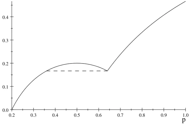
Figure 4: “Ironing” in nested market with 1 = 1=2, 2 = 4=5, 3 = 1
The reason why the largest …rm has non-convex price support can be explained as
one can calculate that the three CDFs increase inp for prices just abovep0, the minimum price. (This is ensured by condition (11).) One can also calculate the smallest price, p1 say, at which some CDF reaches 1 and above which the two remaining …rms compete as
duopolists for prices up to 1. (In the nested case, it is the smallest …rm’s CDF which …rst
reaches 1, although in the general model more detailed analysis is required to determine
which …rm …rst drops out.)
However, in some cases—in the nested case those covered by part (ii) of Proposition
3—the least competitive …rm’s candidate CDF (i.e., when we ignore the monotonicity
constraint on the CDF) starts to decrease in p before the largest CDF reaches 1, which
cannot therefore be a valid CDF. Figure 4 illustrates an example with nested reach where
1 = 1=2, 2 = 4=5 and 3 = 1, and the solid curve depicts the largest …rm’s candidate CDF if we ignored its monotonicity constraint. The correct CDF for the largest …rm is
then obtained by “ironing” this curve as shown on the …gure, so that the largest …rm does
not choose prices in the interval denoted by the dashed line, which from (15)–(16) is the
interval (9=25;16=25) in this example. This procedure is valid as long as the decreasing
candidate CDF does not become negative before the largest CDF reaches 1, and this is
ensured by the condition 2 > 3 in Proposition 3 (or more generally by condition (11) in Proposition 2). As 3= 2 !1, this gap in the least competitive …rm’s support widens, until eventually this …rm does not compete using low prices at all.
The equilibria with “ironing”—when one …rm’s price support has a gap in the middle—
provide insight into the relationship between the two parts of Proposition 2. As the nested
example in Proposition 3 illustrates, as parameters move from satisfying (11) towards
satisfying (12), an equilibrium with ironing emerges, and the lower element of the price
support of the …rm in question shrinks until it disappears, leaving an equilibrium of the
overlapping duopoly form.
5
A model with capacity constraints
As discussed in the introduction, another circumstance in which …rms have limited reach is
when they have capacity constraints, as in the Bertrand-Edgeworth model of competition.
A natural question is how equilibria in this scenario compare with equilibria in our main
model with consideration sets. To address this question in the most direct way we assume
(which avoids the need to posit a particular rationing rule). As we explain, for some con…gurations of capacities (and always when there are just two …rms), equilibria in the
Bertrand-Edgeworth model resemble those that arise in the model with consideration sets.
But for other con…gurations they are quite unlike any such equilibria.
Suppose there is a continuum population of identical consumers of measure 1 who
each consider all prices and are willing to pay 1 for a unit of homogeneous product. Firm
i= 1;2;3can costlessly supply any quantity up to its capacity i but cannot supply beyond
this. A consumer tries to buy at the lowest available price, but is not always able to do
so: once the capacity of the cheapest …rm is exhausted, remaining consumers then try to
buy from the second cheapest …rm, and then any remaining consumers buy from the third …rm.
We make the following assumptions about capacities:
0< 3 2 1 <1 ; (17)
1+ 2+ 3 1>0 ; (18)
2+ 3 <1 : (19)
Condition (17) re‡ects our labelling convention in this section, and has the substantive
assumption that no …rm can supply all consumer demand on its own.18 Here,
i is …rmi’s
supply when it o¤ers a price below both its rivals, and corresponds to “reach” in our main
model. In (18) is the excess of total capacity over demand, and unless it is positive there
is no competition between …rms and the equilibrium price for each …rm is p 1. Firm i’s
supply if it o¤ers a higher price than both its rivals is1 j kif this is positive, and this
represents the …rm’s captive customers. (Since > 0, a …rm is not capacity constrained
when undercut by both rivals, and can only supply its residual demand1 j k, if any.)
Firm i has captive customers if and only if i > , and (19) ensures that the largest …rm
has captive customers (otherwise equilibrium involves all …rms choosing the price p 0).
It is convenient to focus on a …rm’s “contested” customers, de…ned to be its capacity
minus is captive customers, and for …rmi denote this by
i = i maxf1 j k;0g= minf i; g:
18The situation where one …rm has capacity to serve all demand is analyzed as Case 1 in Hirata (2009),
Note that 3 2 1 = . Firm i’s captive-to-reach ratio is 1 i= i, so that
3 2 1, and unlike the consideration set framework here …rms are necessarily or-dered so that …rms with large reach have a large captive-to-reach ratio. Dasgupta and
Maskin (1986) ensures existence of equilibrium in this Bertrand-Edgeworth market, while
[image:25.595.202.402.208.405.2]our earlier Lemma 1 continues to apply.
Figure 5: Interpreting the capacity model in terms of consideration sets
When its rivals use CDFs Fj and Fk to choose their prices, …rmi’s expected sales with
price p 1is
qi = FjFk( i i) + (1 Fj)(1 Fk) i
+(1 Fj)Fkminf i;1 kg+Fj(1 Fk) minf i;1 jg :
For instance, if …rmj undercuts …rm i and …rmk does not, …rmi can supply the residual
demand1 j or its capacity i, whichever is the smaller. Noting that
minf i;1 jg= i + minf ;1 j ( i )g= i + k ;
we can rewrite this expression for qi as
qi = i+ [2 1 2 3]FjFk [ j]Fj [ k]Fk :
Comparing this expression to (9) shows that this market is equivalent to a market with
consideration sets where …rmi has i i captive customers, [ i+ j ]customers who
customers who consider both rivals. Noting that 1 = and that 1 1 = 1 2 3, this demand system can be depicted as the Venn diagram shown on Figure 5, where the
weights in the segments sum to total demand 1.
Here, the term 2+ 3 is strictly positive.19 Therefore, the consumer segment which “considers” all three …rms hasnegative weight 2 3 <0, and this crucial di¤erence with the consideration set model can a¤ect the structure of equilibrium. In particular, with
three …rms the capacity model is never isomorphic to a model with consideration sets.
As with expression (10), …rm i’s demand can be written succinctly as
qi(p) = i[1 + ^GjGk ^ijGj ^ikGk]; (20)
where Gj(p) jFj(p), and
^12 = 3 1 2
; ^13 = 2
1 3
; ^23= 0 and ^ = 2 3
1 2 3
: (21)
Here, ^12 ^13 ^23 = 0. Therefore, using the terminology from section 4, it is the
two largest …rms which have the greatest competitive interaction. The following result is
analogous to Proposition 2, and characterizes when it is an equilibrium for all …rms to
price low.
Proposition 4 (i) If ^12 = ^13 then in equilibrium all …rms have the same minimum price
p0 = (1 2 3)= 1, which is the captive-to-reach ratio of the largest …rm.
(ii) If ^12 > ^13 then in equilibrium only the two largest …rms o¤er the lowest price p0,
which again is the captive-to-reach ratio of the largest …rm.
There are just two ways to achieve the condition ^12 = ^13. Either ^12 = ^13 = 0, in
which case all three …rms have captive customers.20 Alternatively, ^12 = ^13 > 0, when
neither …rm 2 or 3 has captive customers, which requires 2 = 3 so that the two smaller …rms are exactly the same size. Therefore, if …rm 3 has no captive customers and is strictly
smaller than …rm 2, part (ii) of the proposition applies.
Part (ii) does not characterize the smallest …rm’s pro…t or the equilibrium strategies.
However, in the earlier version of this paper (Armstrong and Vickers, 2018, Proposition 3)
19Since
i= minf i; g, the only way the term could be negative is if both 2 and 3 were below , in
which case 2+ 3 = 2+ 3 , which is positive since 1<1.
20It is straightforward to extend this result—that when even the smallest …rm has captive customers
we calculated an equilibrium (for which we did not show uniqueness) whenever part (ii) applied. In that equilibrium the two largest …rms have price support in the whole range
[p0;1], while the smallest …rm chooses it price from a strictly interior interval [p0; p00], where
p0 < p0 < p00 <1. Thus the smallest …rm obtains strictly greater pro…t per unit of capacity than its larger rivals. This pattern of pricing is not possible in the main model with
con-sideration sets, where the only possibilities were for all …rms to price low or for there to be
overlapping duopoly. Conversely, one can show that the overlapping duopoly pattern isnot
possible in this capacity model.21 Thus the segmented price competition sometimes seen in
the consideration sets framework does not appear with Bertrand-Edgeworth competition.22
Another contrast with the main model is that here it is not possible that entry into a duopoly market can harm consumers. To see this, consider two incumbents, A and B,
with respective capacities A and B A. If A+ B 1 then there is no competition
between these …rms, consumers have zero surplus, and entry can only improve consumer
surplus. Suppose then that A+ B > 1, so that the incumbents cover the market, in
which case industry pro…t without entry (as in expression (2) above) is
( A+ B)
1 B
A :
Suppose a third …rm enters, with capacity E. Since demand was already met, entry
leaves welfare unchanged and consumers are harmed if and only if industry pro…t rises.
If E 1 B then no …rm has any captive customers after entry, equilibrium price is
p 0 and consumers bene…t from entry. Otherwise, if E < 1 B …rm A has captive
demand but …rm E does not. In the knife-edge case where E = B, part (i) applies, and
a direct calculation shows that industry pro…t falls. If E < B, so that the entrant is the
smallest …rm, part (ii) applies with minimum price p0 = (1 B E)= A. If E denotes 21If an overlapping duopoly equilibrium did exist, part (ii) of Proposition 4 applies so …rm 3 has no
captive customers and …rms 1 and 2 price low. There would then be a threshold price p1 which is …rm
2’s highest price and …rm 3’s lowest price. Since …rm 3 has no captive customers, its demand at p=p1
is 3(1 F1(p1)), and since it cannot be better o¤ with pricep=p0, we require that1 F1(p1) p0=p1.
However, the fact that …rm 2 is willing to choosep1implies that1 F1(p1)< p0=p1, which is a contraction.
22Unlike our main model with consideration sets, in the capacity framework our assumption of unit
the entrant’s pro…t, the change in pro…t due to entry is
( A+ B)p0 + E ( A+ B)
1 B
A
= E E
A+ B
A :
However, the entrant cannot make pro…t greater than E (which is its pro…t if it could
supply its capacity at price p = 1), and so the above change in pro…t is negative and
consumers bene…t from entry. Finally, if B < E < A, so the entrant is the middle …rm,
then …rm B also has no captive customers, and part (ii) applies with the same minimum
price p0 = (1 B E)= A. The change in pro…t due to entry is now
( A+ E)p0+ B ( A+ B)
1 B
A
( A+ E)p0+ B ( A+ B)
1 B
A
= (1 A B)( E B) 2
E
A
<0 :
Here, the …rst inequality follows since B B, and the second inequality follows since
the entrant has no captive customers.
More generally, our main model with consideration sets allows for richer patterns of
competition interaction than the Bertrand-Edgeworth model. In the former framework, entry can occur without reducing the number of captive customers, a …rm can have di¤erent
“overlap” with similarly-sized rivals, and a small …rm can have a high proportion of its
reach captive, none of which are possible in the capacity framework.
6
Conclusions
The aim of this paper has been to explore, in a parsimonious framework with price-setting
…rms and homogeneous products, how patterns of consumer consideration matter for
com-petitive outcomes, in particular the nature of price dispersion in mixed-strategy equilibria. The analysis has yielded a number of results that we did not initially expect. First, whereas
in existing models all …rms are direct competitors over a range of prices, we found equilibria
with segmented pricing patterns, i.e., with some …rms only pricing high and others only
pricing low.
Second, in the three-…rm case we established generically either that all …rms set the
same minimum price (in which case their pro…t was proportional to reach), or that pricing
was segmented (so that one …rm only set low prices and one set only high prices). In prior
on the knife edge between these two regimes. Third, the key to determining which of the two regimes applies was found to be the proximity or otherwise of the pairwise correlation
measures of competitive interaction, ij, and when one pair of …rms had signi…cantly greater
competitive interaction than other pairs then segmented pricing ensued. Fourth, for some
parameter con…gurations we found equilibria with a gap in one …rm’s price support, so
that that …rm sometimes prices high, and sometimes low, but never in between.
Fifth, we found plausible patterns of consumer consideration in which entry is
detri-mental to consumers because it softens competition between incumbents, leading them to
retreat to exploit their captive consumers. Likewise, there were situations where an increase
in the number of consumers who consider one pair of …rms causes a third …rm to retreat towards its captive base, showing that search externalities need not bene…t all consumers.
Sixth, our model of competition with consumer consideration sets can di¤er radically from
the familiar Bertrand-Edgeworth model of competition with capacity constraints. Indeed
in the three-…rm case the latter can be interpreted as consideration set model in which
a negative proportion of consumers consider all of the …rms. This di¤erence implies that
overlapping duopoly pricing is not a feature of the Bertrand-Edgeworth model.
The analysis could be extended in two broad directions. One would be to settings
beyond nested reach and the three-…rm case that we have analysed in detail. For example, one could seek more general conditions for equilibrium to take the overlapping duopoly
form, or one could try to establish that all …rms use the same minimum price when pairwise
competitive interactions are similar enough. The other approach would be to endogenise
the pattern of consideration sets, beyond our analysis of entry and mergers, by introducing
search by consumers and/or advertising by …rms.23 For instance, one could study a model
of non-sequential search where a consumer can choose her consideration set S …rms by
incurring a speci…ed up-front search cost (increasing in S). Such a framework would
generalize Burdett and Judd (1983, section 3.2) to allow …rms to be asymmetric and for
consumers to target speci…c …rms for consideration.
23For instance, in the context of advertising, Ireland (1993) and McAfee (1994) study a sequential model
References
Armstrong, M., and J. Vickers (2018): “Patterns of Competition with Captive
Cus-tomers,” Department of Economics Working Paper No. 864, University of Oxford.
(2019): “Discriminating Against Captive Customers,” American Economic
Re-view: Insights, forthcoming.
Baye, M., D. Kovenock,and C. De Vries(1992): “It Takes Two to Tango: Equilibria
in a Model of Sales,”Games and Economic Behavior, 4, 493–510.
Baye, M., and J. Morgan (2001): “Information Gatekeepers on the Internet and the
Competitiveness of Homogeneous Product Markets,”American Economic Review, 91(3),
454–474.
Bulow, J., and J. Levin (2006): “Matching and Price Competition,” American
Eco-nomic Review, 96(3), 652–668.
Burdett, K., and K. Judd (1983): “Equilibrium Price Dispersion,” Econometrica,
51(4), 955–969.
Butters, G.(1977): “Equilibrium Distributions of Sales and Advertising Prices,”Review
of Economic Studies, 44(3), 465–491.
Chen, Y.,and M. Riordan (2007): “Price and Variety in the Spokes Model,”Economic
Journal, 117, 897–921.
(2008): “Price-Increasing Competition,”Rand Journal of Economics, 39(4), 1042–
1058.
Chioveanu, I., and J. Zhou (2013): “Price Competition with Consumer Confusion,”
Management Science, 59(11), 2450–2469.
Dasgupta, P., and E. Maskin (1986): “The Existence of Equilibrium in Discontinuous
Economic Games, I: Theory,” Review of Economic Studies, 53(1), 1–26.
De Francesco, M., and N. Salvadori (2015): “Bertrand-Edgeworth Games Under
Hirata, D.(2009): “Asymmetric Bertrand-Edgeworth Oligopoly and Mergers,”The B.E.
Journal of Theoretical Economics (Topics), 9(1).
Honka, E., A. Hortacsu, and M. A. Vitorino (2017): “Advertising, Consumer
Awareness, and Choice: Evidence From the U.S. Banking Industry,” Rand Journal of
Economics, 48(3), 611–646.
Inderst, R. (2002): “Why Competition May Drive up Prices,” Journal of Economic
Behavior and Organization, 47(4), 451–462.
Ireland, N.(1993): “The Provision of Information in a Bertrand Oligopoly,” Journal of
Industrial Economics, 41(1), 61–76.
Janssen, M., and E. Rasmusen (2002): “Bertrand Competition Under Uncertainty,”
Journal of Industrial Economics, 50(1), 11–21.
Manzini, P., and M. Mariotti (2014): “Stochastic Choice and Consideration Sets,”
Econometrica, 82(3), 1153–1176.
McAfee, R. P.(1994): “Endogneous Availability, Cartels, and Merger in an Equilibirium
Price Dispersion,” Journal of Economic Theory, 62, 24–47.
Montez, J., and N. Schutz (2019): “All-pay Oligopolies: Price Competition with
Unobservable Inventory Choices,” mimeo.
Narasimhan, C.(1988): “Competitive Promotional Strategies,”Journal of Business, 61,
427–449.
Piccione, M., and R. Spiegler (2012): “Price Competition Under Limited
Compara-bility,” Quarterly Journal of Economics, 127(1), 97–135.
Prat, A. (2018): “Media Power,”Journal of Political Economy, 126(4), 1747–1782.
Rosenthal, R. (1980): “A Model in which an Increase in the Number of Sellers Leads
to a Higher Price,”Econometrica, 48(6), 1575–1579.
Smith, H. (2004): “Supermarket Choice and Supermarket Competition in Market
Sovinsky Goeree, M. (2008): “Limited Information and Advertising in the U.S.
Per-sonal Computer Industry,”Econometrica, 76(5), 1017–1074.
Spiegler, R. (2006): “The Market for Quacks,” Review of Economic Studies, 73(4),
1113–1131.
(2011): Bounded Rationality and Industrial Organization. Oxford University Press,
Oxford, UK.
Szech, N.(2011): “Welfare in Markets where Consumers Rely on Word of Mouth,” mimeo.
Varian, H.(1980): “A Model of Sales,” American Economic Review, 70(4), 651–659.
Vives, X. (1999): Oligopoly Theory: Old Ideas and New Tools. MIT Press, Cambridge.
Technical Appendix
Sketch proof of Lemma 1: We …rst discuss arguments to do with deletion of dominated
prices. In any equilibrium we have i i, since …rm i can ensure at least this pro…t by
choosing price equal to 1 and serving its captive customers. For this reason, no …rm would
ever o¤er a price below i, its captive-to-reach ratio, since if it did so it would obtain pro…t
below i even if it supplied its entire reach.
To see that every …rm makes positive pro…t we invoke Assumption 2. There is at least
one …rmiwhich has captive customers, and which will not set price below i >0. (Clearly
this …rm makes positive pro…t.) From the remaining …rms, at least one …rm j has captive
customers in the subset of …rms excluding i, and so this …rm can set price i and be sure
to obtain positive pro…t. Firm j therefore also has a positive lower bound on its prices.
Following the same argument, a …rm in the subset of …rms excluding both i and j can
obtain positive pro…t, and so on until the set of …rms is exhausted. In particular, each
…rm’s minimum price is strictly above zero and hence so is p0. This proves part (ii). If pricep < 1is in …rm i’s support thenqi( )in (1) cannot be ‡at for prices just above p, for otherwise the …rm would obtain strictly greater pro…t by raising its price above
p. This implies that this price must be in the support of at least one other …rm. More
precisely, if price p < 1 is in …rm i’s support it must be in the support of at least one of
its “potential competitors”, where in a given equilibrium we say that …rmj is a “potential
i at price p given the equilibrium strategies followed by …rms other than i and j. (This then implies that i is a potential competitor for j.) If for all duopoly segments we have
ij > 0, then every …rm is a potential competitor for every other …rm. However, two
…rms might have disjoint reaches, and so cannot be potential competitors. More generally,
the overlap between i and j might be contained within a third …rm’s reach, and if in the
equilibrium the third …rm always chooses price below p, then i and j do not compete at
price p. If price pin …rmi’s support wasnot in the support of at least one of its potential
competitors, …rmi’s demand would be ‡at (and positive) in this neighbourhood ofp, which
is not compatible with pmaximizing the …rm’s pro…t.
We next turn to arguments concerning the possibility of “atoms” in the price distri-butions. First observe that two …rms cannot both have an atom at price p if they are
potential competitors at this price (for otherwise each would have an incentive to undercut
the price p and gain a discrete jump in demand).
To see that each …rm’s price distribution is continuous in the interval [p0;1), suppose by contrast that …rmi has an atom at some price0< p < 1in its support. We claim that
…rm’s idemand in (1) must then be locally ‡at above p. As noted above, there cannot be
a potential competitor toiat pricepwhich also has an atom atp, and soqi does not jump
down discretely at p. In addition, any potential competitor to i at p obtains a discrete increase in demand if it slightly undercutsp, and so such a …rm would never choose a price
immediately above p. Since no potential competitor chooses a price immediately abovep,
…rmi loses no demand if it raises its price slightly above p, which is not compatible with
p maximizing the …rm’s pro…t. Therefore, …rm i cannot have an atom below 1, and this
completes the proof of part (iii). This implies that each …rm’s demand (1) is continuous
in the interval [p0;1).
Similarly, if p0 is the minimum price ever chosen in the market, then all prices in the interval [p0;1] are sometimes chosen. Ifp is in …rm i’s support but no …rm is active in an interval(p; p0)above p, then …rm ihas ‡at demand over the range (p; p0), and this cannot
occur in equilibrium. This completes the proof of part (iv).
Suppose now that there are at least three …rms. Let Pij denote the set of prices in