World Resources Determine World Prices

Munich Personal RePEc Archive

World Resources Determine World Prices

Guo, Baoping

Individual Researcher

November 2017

Online at

https://mpra.ub.uni-muenchen.de/91095/

1

World Resources Determine World Prices

Baoping Guo1

Abstract –This paper derived a general equilibrium of the Heckscher-Ohlin model for the context

of two-factor, multiple-commodity, and multiple-country (2 x N x M model). The equalized factor

price (PFE) and world commodity price at the equilibrium are just the prices Dixit and Norman

predicted, that the prices from equilibriums remains the same when the allocation of factor

endowments changes within (the 2 x N x M) IWE box. The study shows how price-trade

equilibriums reached for multiple countries and how world prices was determined. The

equilibrium and world price structure shows that world (factor endowments) resources

determine the world price. This is another core understanding of international trade.

Keywords:

IWE; Factor price equalization; Heckscher-Ohlin; Equilibrium price; equalized factor price; Dixit-Norman

1. Introduction

There are many important literatures on general equilibriums of trade and the factor price equalizations. Samuelson’s factor-price equalization theorem is a remarkable result. McKenzie (1955)’s cone of diversification of factor endowments is an important concept to understand the necessary condition of general equilibrium.

Vanek(1968)’s HOV model linked prices with trade and consumption by using shares of GNP. It also resulted in the application issue how to convert the assumption of homothetic taste into consumption balance.

Jones(1965) provided the popular system equations for the Heckscher-Ohlin model, which allowed costs going with productions smoothly and lightly.

1 _{Former faculty member of College of West Virginia, corresponding address: 8916 Garden Stone Lane, Fairfax, VA 22031,}

2

Either (1984) discussed the generalization of the Heckscher-Ohlin theories in higher-dimensional contexts. David Gale and H. Nikaio (1965) provided conditions to guarantee global univalence of factor price and commodity price by an input-output matrix that is a matrix with all positive principal minors.

Dixit and Norman (1980) provided a strong clue for what a price-trade equilibrium should be and what an equalized factor price is. It draws out unique characteristic of equalized factor price under IWE diagram.

Wu (1987) discussed the equalization of factor prices in general equilibrium when commodities outnumber factors. Woodland (2011) mentioned that from a theory perspective, factor price equalization is a prediction of the model rather than an assumption. He summarized all-important achievements in the studies of general equilibriums.

Helpman and Krugman (1985) provide a formal definition of FPE set in higher dimensions. Deardroff (1994) studied the possibility of factor price equalizations. His endowment lenses with six goods and five countries are very impressive to understand the issues.

Guo (2005) started his researches of the structure of FPE price by using the term of trade and shares of GNP. Guo (2018) presented a solution of general equilibrium of trade on the Heckscher-Ohlin 2 x 2 x 2 model. He demonstrated that the equalized factor price is quantitatively available for a giving IWE box. This is an interesting result to understand where trade equilibriums reach and what a structure an equalized factor price is.

This study generalized the Guo (2018) result. It demonstrates that general equilibriums and equalized factor prices are available for the Heckscher-Ohlin 2 x N x M frameworks. The

equilibriums are just also the Dixit-Norman’s integrated world equilibrium. The equalized factor price and common commodity price will remain the same when the allocations of factor

endowments change in the IWE box.

3

This paper is divided into five sections. Section 2 reviews the general equilibrium of trade (Guo 2018) and the price structure at the equilibrium. Section 3 derives a general equilibrium of trade for models with two factors, two commodities, and multiple countries (2 x 2 x M). Section 4 examines the 2 x N x M model. It provides equilibrium solutions for more general cases. Section 5 discusses a new understanding of international economics that world resources determine world price, under the market mechanism of commodity trade.

2. Review of the Equalized Factor Price from Integrated World Equilibrium (IWE)

With the normal assumptions of the Heckscher-Ohlin theory, Guo (2018) denoted a standard 2 x 2x 2 model in the following way:

a. The production constraint of full employment of resources are

𝐴𝑋ℎ _{= 𝑉}ℎ _{(ℎ = 𝐻, 𝐹) (2-1)}

where A is the 2x2 technology matrix, 𝑋ℎ is the 2 x1 vector of commodities of country h, 𝑉ℎ is the 2x1 vector of factor endowments of country h. The elements of matrix A is 𝑎_𝑘𝑖(𝑊), 𝑘 = 𝐾, 𝐿, 𝑖 = 1,2.

b. The zero-profit unit cost condition is

𝐴′_𝑊∗ _{= 𝑃}∗ _(2-2)

where 𝑊∗is the 2x1 vector of factor prices, 𝑃∗ is the 2x1 vector of commodity prices. Both 𝑃∗ and 𝑊∗ _{are world price when factor price equalization happened, its elements are 𝑟}∗ _{rental and 𝑤}∗

wage.

c. The definition of the share of GNP of country ℎ to world GNP,

𝑠ℎ _{= 𝑃}′ _𝑋ℎ_/𝑃′ _𝑋𝑊 _{(ℎ = 𝐻, 𝐹) (2-3)}

d. The trade balance condition is

𝑃′ _𝑇ℎ _{= 0 (ℎ = 𝐻, 𝐹) (2-4)}

or

𝑊′ 𝐹ℎ = 0 (ℎ = 𝐻, 𝐹) (2-5) where 𝑇ℎis a 2x1 vector of commodity export, 𝐹ℎ is a 2x1 vector of factor content of trade.

e. The constraint of the cone of diversification of factor endowments

𝑎_𝐾1 𝑎_𝐿1 >

𝐾𝐻

𝐿𝐻 >

𝑎_𝐾2

𝑎_𝐿2 𝑎_𝐾1 𝑎_𝐿1 >

𝐾𝐹

𝐿𝐹 >

𝑎_𝐾2

𝑎_𝐿2 (2-6)

f. The constraint of commodity price limits2

𝑎𝐾1

𝑎_𝐾2 > 𝑝1∗

𝑝₂∗ > 𝑎_𝑎𝐿1

𝐿2 (2-7)

2 _{This condition will guarantee all possible factor prices are positive. We may refer (7) to the constraint of cone of}

4

The model takes the normal Heckscher-Ohlin assumptions as (1) identical technology across countries, (2) identical homothetic taste, (3) perfect competition in the commodities and factors markets, (4) no cost for international exchanges of commodities, (5) factors are completely immobile across countries but that can move costlessly between sectors within a country, (6) constant return of scale and no factor intensity reversals, and (7) full employment of factor resources.

By using a simple competitive home country’s GNP share as3

𝑠ℎ₌1 2

𝐾𝐻𝐿𝑤+𝐾𝑤𝐿𝐻

𝐾𝑤_𝐿𝑤 (2-8) where superscript w indicates the factor endowment is the world factor endowment and 𝑠ℎ is country home’s share of GNP to world GNP.

Guo (2018) obtained the general equilibrium of trade of the Heckscher-Ohlin model as

𝑟∗ 𝑤∗ =

𝐿𝑤

𝐾𝑤 (2-9)

𝑤∗ _{= 1 (2-10)}

𝑝1∗= 𝑎𝑘1𝐿

𝑤

𝐾𝑤 + 𝑎𝐿1 (2-11) 𝑝2∗ = 𝑎𝑘2 𝐿

𝑤

𝐾𝑤+ 𝑎𝐿2 (2-12) 𝐹𝐾𝐻= 1₂𝐾

𝐻_𝐿𝑤_−𝐾𝑤_𝐿𝐻

𝐿𝑤 (2-13)

𝐹_𝐿𝐻 = 1

2

𝐾𝐻𝐿𝑤−𝐾𝑤𝐿𝐻

𝐾𝑤 (2-14)

All the endogenous price variables 𝑝₁∗ , 𝑝₂∗ , 𝑤∗ , 𝑟∗ in the model are expressed by exogenous variables (𝐾𝑤, 𝐿𝑤).

It shows that Samuelson’s equalized factor price at the equilibrium is just the Dixit-Norman’s IWE factor price. Dixit and Norman (1980) illustrated that if the allocation of the factor endowments in the IWE box changes, the factor price and the commodity price will remain same. The price

solution just reflects that.

The factor content of trade in (2-13) and (2-14) restates the Heckscher-Ohlin theorem. It says that

if 𝐾_𝐿𝐻𝐻 > 𝐾_𝐿𝑤𝑤 , then 𝐹_𝐾𝐻 > 0.

For a giving IWE box, the solution of the equilibrium is unique since there is only one trade equilibrium point in IWE diagram.

3 _{Guo used a simple utility function to maximize each country benefits with trade box, to achieve this share of GNP, we will}

5

We will use the same approach in next section to address the multi-nation issue.

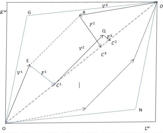
3. General Equilibrium of trade for the case of two factors, two commodities, and multiple countries

Figure 1 draws an IWE diagram for two factors, two commodities, and three countries. In this diagram, 𝑉ℎ(𝐿ℎ, 𝐾ℎ) represents the vector of factor endowments of country ℎ, h=1, 2, and 3. We can observe three trade points 𝐶1, 𝐶2, and 𝐶3 for each countries accordingly.

3.1 trade partner for a country

In a two-country system, home and foreign, they are trade partners each other. In a 3-country system, country 1, country 2, and country 3, who is the trade partner for whom? We specify that trades here are one that a country trade with the rest of the world. We do not talk about the trade in which country 1 trade with country 2 or with country 3. We talk about that country 1 trade with the rest of the world. The trade relations now are very simple; it just likes the scenario of the two-country system.

6

productive factors. Usually identified in theory textbooks as land, labor, and capital.” He stated what a trade means in a multiple-nation system, from the view of the Heckscher-Ohlin model.

Figure 2. is an IWE diagram which shows how a country trades with the rest of the world. In addition, the boundaries of shares of GNP are added to the diagram.

The factor endowment vector 𝑉1 of country 1 is arranged to start at origin point O. The rest of the world factor endowment is 𝑉2 +𝑉3, they starts at the origin point 𝑂′.

The algebra expression for the 2 x 2 x M model is as same as equation (1)-(6); the only difference is the country number. The country number now goes from 1 to 3.

3.2 Identifying the trade box

Trades will redistribute national welfares, which are measured by GNPs. The GNP is a function of price.

7

Using 𝑝₁∗ = 𝑎_𝐾1 and 𝑝₂∗ = 𝑎_𝐾2 in the definition of GNP (2-3), we obtain the first boundary of country 1’ share of GNP as

𝑠𝑏1 = 𝐾

1

𝐾𝑤 (3-1) Similarly, using 𝑝₁∗= 𝑎_𝐿1 and 𝑝₂∗ = 𝑎_𝐿2 , we obtain another boundary of country 1’s share of GNP boundary as

𝑠_𝑎1 = 𝐿1

𝐿𝑊 (3-2) Assuming country 1 is capital abundant as

𝐾1 𝐿1 >

𝐾2+𝐾3

𝐿2_+𝐿3 (3-3) The boundaries of country 1’s share of GNP satisfy

𝑠𝑏1 = 𝐾

1

𝐾𝑤> 𝑠1 > 𝑠𝑎1 =

𝐿1

𝐿𝑤 (3-4) They are indicated on the horizontal unity axis.

When 𝑠 → 𝐾1

𝐾𝑤 there are

𝑝1∗

𝑝₂∗ =𝑎_𝑎𝐾1_𝐾2, 𝑟∗ =_𝑎1_𝐾2 , 𝑤∗ = 0 (3-5) and when 𝑠 → 𝐿1

𝐿𝑤 there are

𝑝_𝑝1∗ 2∗ =

𝑎𝐿1

𝑎𝐿2, 𝑟

∗ _{= 0 , 𝑤}∗ ₌ 1

𝑎𝐿2 (3-6) So the commodity price limits are

𝑎𝐾1

𝑎𝐾2 >

𝑝₁∗

𝑝₂∗ > 𝑎𝐿1

𝑎𝐿1 (3-7)

And the wage and rental limits are:

1 𝑎𝐾2 >𝑟

∗ _{> 0 (3-8)}

0 < 𝑤∗ _< 1

𝑎𝐿2 (3-9) Prices4 _{from equilibriums should be limited by (3-7) through (3-9)}

The factor endowment allocation is at point E, where country 1 is capital abundant.

We refer to the area EUQR as the trade box. Line E𝐶1 indicates a trade. It can measure the factor contents of trade as

𝐹𝐾1 = 𝐾1 − 𝑠1𝐾𝑤 (3-10)

𝐹𝐿1 = 𝐿1 − 𝑠1𝐿𝑤 (3-11)

By trade balance (3-10), the term of factor content of trade is the relative factor price as

𝑟 𝑤 = −

𝐿1−𝑠1𝐿𝑤

𝐾1−𝑠1𝐾𝑤 (3-12)

4 _{Prices here are relative prices referring 𝑝}

8

If we know 𝑠1, we can obtain the relative factor price and trade amounts.

3.3 Settling trade equilibrium point

The country 1’ s share of GNP 𝑠1 divides the trade box into two parts. Their lengths are 𝛼 and 𝛽, separately. When 𝛼 increases, the countr 1’s share of GNP increases and the rest of the world’s share of GNP decreases, and vice versa. In trade competitions, the both sides want to reach their maximum GNP shares through free trade.

We need to ware that only trade box is the redistribution area of shares of GNP for the economy. Outside the box, they are not redistributable. There are no right commodity prices reaching them. This is an essential meaning of boundaries of shares of GNPs.

From Figure. 3, the length of 𝛽 can be expressed as

𝛽 = 𝑠𝑏1− 𝑠𝑎1− 𝛼 (3-13)

When 𝛼 = 𝛽 , both countries reach their maximum values of GNP shares in the trade box; the country 1’s share of GNP now is

𝑠1 = 𝛼 + 𝑠_𝑎1 = 1

2(𝑠𝑏1+ 𝑠𝑎1) (3-14)

Substituting (3-1) and (3-2) into (3-14) yields

𝑠1=1

2

𝐾1𝐿𝑤+𝐾𝑤𝐿1

𝐾𝑤𝐿𝑤 (3-15)

We can also interpret the result as that the best welfares of two countries should avoid the hurts of extreme trade points by 𝑠_𝑏1, 𝑠_𝑎1 as far as possible. When taking the share of GNP as 𝑠_𝑏1, then 𝑤∗ _{= 0; and when taking the share of GNP as 𝑠}

𝑎1, then 𝑟∗= 0. The middle point is the best position

to reward both factors fairly based on existing factor endowment supplies.

3.4 General equilibrium

Substituting equation (3-15) into (3-12), we can get the relative factor price ratio as

𝑟∗1 𝑤∗1 =

𝐿𝑤

𝐾𝑤 (3-16)

We can also get commodity price and export vector accordingly by equation 10) through (2-12).

3.5 The price solution is the same for all countries

9

𝑟∗2 𝑤∗2 =

𝐿𝑤

𝐾𝑤 (3-17)

This means that the relative factor price is the same for all countries.

𝑟∗1 𝑤∗1 =

𝑟∗2 𝑤∗2 =

𝐿𝑤 𝐾𝑤 =

𝑟∗

𝑤∗ (3-18) In addition, trade angle θ is the same for all countries. The shares of GNP will be different from country to country.

By assuming 𝑤∗= 1 to drop one market-clearing condition by Walras’s equilibrium, we obtain

𝑠1=1₂𝐾ℎ𝐿_𝐾𝑤_𝑤+𝐾_𝐿𝑤𝑤𝐿ℎ (ℎ = 1,2,3) (3-19)

𝑟∗ 𝑤∗ =

𝐿𝑤

𝐾𝑤 (3-20) 𝑤∗ _{= 1 (3-21)}

𝑝1∗= 𝑎𝑘1𝐿

𝑤

𝐾𝑤 + 𝑎𝐿1 (3-22) 𝑝2∗ = 𝑎𝑘2 𝐿

𝑤

𝐾𝑤+ 𝑎𝐿2 (3-23) 𝐹𝐾ℎ =1₂𝐾

ℎ_𝐿𝑤_−𝐾𝑤_𝐿ℎ

𝐿𝑤 (ℎ = 1,2,3) (3-24)

𝐹_𝐿ℎ = −1

2

𝐾ℎ𝐿𝑤−𝐾𝑤𝐿ℎ

𝐾𝑤 (ℎ = 1,2,3) (3-25)

Those are the equilibrium solution for the 2 x 2 x 3 model.

3.5 A numerical example

Let see a numerical example for a three-country economy. The technology matrix is [𝑎_𝑎𝐾1 𝑎𝐾2

𝐿1 𝑎𝐿1] = [3 11 2]

Commodity 1 is capital intensive. The factor endowments for three countries are [𝐾1

𝐿1] = [5000_4500], [𝐾 2

𝐿2] = [6000_4500], [𝐾 3

𝐿3] = [4500_5500]

By using factor abundance definition𝐾 ℎ

𝐾𝑤 > 𝐿ℎ

𝐿𝑤, country 1 and country 2 is capital abundant;

country 3 is labor abundant. Country 1 and country 2 will export commodity 1 and country 3 will export commodity 2. The commodity outputs of three countries by the full employment of factor resources separately as

[𝑥_𝑥11

21] = [11001700], [𝑥 12

𝑥22] = [15001500], [𝑥 13

𝑥23] = [ 7002400]

The correspondent limits of share of GNP of each country separately are 𝑠1𝑏 = 0.3225 > 𝑠1 > 𝑠1𝑎 = 0.2903

10

𝑠3𝑏 = 0.2903 > 𝑠3 > 𝑠3𝑎 = 0.3870

The shares of GNP of three countries separately are 𝑠1 = 0.3164

𝑠2 = 0.3487

𝑠3 = 0.3348

The sum of the three countries’ share of GNP is 1.

With those shares of GNP, the consumptions and the export will be

[𝑐11

𝑐21] = [1044.321772.19], [𝑐 12

𝑐22] = [1150.771952.83], [𝑐 13

𝑐23] = [1104.891874.97]

[𝑇1

1

𝑇21] = [ 55.67−72.19], [𝑇 12

𝑇22] = [ 349.22−452.83], [𝑇 13

𝑇23] = [−404.89525.02 ]

[𝐹𝐾

1

𝐹𝐿1] = [ 94.82−88.70], [𝐹 𝐾2

𝐹𝐿2] = [ 594.82−556.452], [𝐹 𝐾3

𝐹𝐿3] = [−669.65645.16 ]

In addition, the common commodity price and the equalized factor price at trade equilibrium are

[𝑝1

∗

𝑝2∗] = [3.80642.9354] , [ 𝑟 ∗

𝑤∗] = [0.9354_{1.000 ]}

4. The case of two factors, multiple commodities, and multiple countries

We cannot determine commodity outputs by factor endowments if the technology matrix is not square (not even). With multiple commodities (N>2), we need to know the commodity output quantities and the amounts of the factor endowments in advance if we start to process any

equilibrium analyses. Deardorff (1994) illustrates that when the allocation of factor endowment is inside the cones, but above the lenses, the factor-equalization is not available. To avoid this

situation, we assume in the following analysis that outputs be positive, that factor resources be of full employment, and that allocations of factor endowments are inside the lenses. We also

emphasize that equations (2-6) and (2-7) is the necessary condition for a price-trade equilibrium.

We still use the basic notations in section 2. The technology matrix for multiple commodities and two factors now is

𝐴 = [𝑎𝑘1 𝑎𝑘2 ⋯ 𝑎𝑘𝑛 𝑎𝐿1 𝑎𝐿2 ⋯ 𝑎𝐿𝑛

] 𝑛 = (1,2, ⋯ , 𝑁) (4-1)

11 𝑃 =

[ 𝑝1ℎ

𝑝2ℎ

⋮ 𝑝𝑛ℎ]

, 𝑋ℎ = [ 𝑥1ℎ

𝑥2ℎ

⋮ 𝑥𝑛ℎ]

ℎ = (1,2, ⋯ , 𝑀) , 𝑛 = (1,2, ⋯ , 𝑁) (4-2)

where ℎ indicates countries.

And factor endowments and factor prices are the 2 × 1 vectors 𝑉ℎ = [𝐾ℎ

𝐿ℎ], 𝑊∗ = [ 𝑟 ∗

𝑤∗] , ℎ = (1,2, ⋯ , 𝑀) (4-3)

To establish the trade equilibrium, we start at finding the boundaries of shares of GNP of country ℎ.

We cannot use equation (2-7) directly to obtain the boundaries of commodity price. Let see it in another way. We rewrite unit cost as the following,

[ 𝑎𝑘1

𝑎𝑘2

⋮ 𝑎_𝑘𝑛]

𝑟∗₊

[ 𝑎𝐿1

𝑎𝐿2

⋮ 𝑎𝐿𝑛]

𝑤∗₌

[ 𝑝1ℎ

𝑝2ℎ

⋮ 𝑝𝑛ℎ]

(4-4)

When 𝑤∗ = 0 , price reaches at its one boundary as

𝑝𝑏 = [ 𝑎𝑘1

𝑎_𝑘2 ⋮ 𝑎𝑘𝑛]

𝑟∗ _(4-5)

Substituting it into GNP function (2-2), we obtain the correspondence GNP boundary value as

𝑠𝑏ℎ(𝑝𝑏) =𝐾

ℎ

𝐾𝑤 ℎ = (1,2, ⋯ , 𝑀) (4-6)

Similarly, using another price boundary as the following,

, 𝑝𝑎 =

[ 𝑎𝐿1

𝑎𝐿2

⋮ 𝑎𝐿𝑛]

𝑤∗ _(4-7)

substituting it into the function of the share of GNP in equation (3) yields

𝑠_𝑎ℎ(𝑝𝑎) =𝐿 ℎ

𝐿𝑤 ℎ = (1,2, ⋯ , 𝑀) (4-8)

The competitive share of GNP of country ℎ, as we discussed in the last section, will be 𝑠ℎ ₌ 1

2(𝑠𝑏ℎ+ 𝑠𝑎ℎ) = 1 2

𝐾ℎ𝐿𝑤+𝐾𝑤𝐿ℎ

𝐾𝑤𝐿𝑤 ℎ = (1,2, ⋯ , 𝑀) (4-9)

With this share of GNP, we obtain factor contents of trade for country ℎ as 𝐹𝐾ℎ =1₂𝐾

ℎ_𝐿𝑤_−𝐾𝑤_𝐿ℎ

𝐿𝑤 ℎ = (1,2, ⋯ , 𝑀) (4-10)

𝐹_𝐿ℎ =1₂𝐾

ℎ_𝐿𝑤_−𝐾𝑤_𝐿ℎ

12 The commodity exports for country h will be

𝑇1ℎ = 𝑥1ℎ−1₂𝐾

ℎ_𝐿𝑤_+𝐾𝑤_𝐿ℎ

𝐾𝑤𝐿𝑤 𝑥1𝑤 ℎ = (1,2, ⋯ , 𝑀) (4-12)

𝑇2ℎ = 𝑥2ℎ−1₂𝐾

ℎ_𝐿𝑤_+𝐾𝑤_𝐿ℎ

𝐾𝑤𝐿𝑤 𝑥2𝑤 ℎ = (1,2, ⋯ , 𝑀) (4-13) The relative factor price for country ℎ can be expressed as

𝑟∗ℎ 𝑤∗ℎ= −

𝐹𝐿ℎ

𝐹_𝐾ℎ=

𝐿𝑤 𝐾𝑤 =

𝑟∗

𝑤∗ ℎ = (1,2, ⋯ , 𝑀) (4-14) Therefore, all countries’ rental-wage ratios are same. Assume world common wage as numerica as 1,

𝑤∗ = 1 (4-15) The common commodity price can be written as

[ 𝑝1∗

𝑝2∗

⋮ 𝑝𝑛∗

] = [ 𝑎𝑘1

𝑎𝑘2

⋮ 𝑎𝑘𝑛

𝑎𝐿1

𝑎𝐿2

⋮ 𝑎𝐿𝑛]

[𝐿 𝑤

𝐾𝑤

1] (4-16)

Equations (4-14) through (4-16) are the price solution of two factors, multiple commodities, and multiple countries. They are an analytical expression of the factor-price equalization theorem.

The solution shows that prices depend on world factor endowments directly, so it is Dixit-Norman IWE price.

We can observe that the sum of the shares of GNP (4-9) of all countries equals 1.

Equations (4-10) through (4-13) are an analytical expression of the Heckscher-Ohlin theorem generalized, in the case of multiple commodities and multiple countries of the two-factor economy.

For the scenario of the non-square matrix (not even), we can get trade amounts of commodities without issues. Once we know the share of GNP of a country, we can get its import and export amounts by using equation (4-10) and (4-13).

Let see a numerical example for two factors, three commodities, and two countries. In this example, the technology matrix is not a square matrix. Therefore, we need to know the output quantities in advance.

13 𝐴 = [𝑎𝑘1 𝑎𝑘2 𝑎𝑘3

𝑎𝐿1 𝑎𝐿2 𝑎𝐿3] = [ 3

1.3 1.2

0.9 2 3 ]

Suppose the commodity outputs are

[𝑥1

𝐻

𝑥2𝐻

𝑥3𝐻

] = [200100 300]

, [ 𝑥1𝐹

𝑥2𝐹

𝑥3𝐹

] = [300200 100] By full employment, the factor endowments for the two countries are

[𝐾𝐻

𝐿𝐻] = [2700_2500], [𝐾 𝐹

𝐿𝐹] = [2400_2600]

The commodity prices are in 3-demission space. When

𝑝𝑏 _{= [}𝑎_𝑎𝑘1 𝑘2

𝑎𝑘3

] = [0.92 3 ] then

𝑠𝑏𝐻 = 0.4599

When

𝑝𝑎_{= [}𝑎_𝑎𝐿1 𝐿2

𝑎𝐿3

] = [1.33 1.2] then

𝑠𝑎𝐻 = 0.5688

The share of GNP of the home country is the average value of above two as 0.5144. With this share of GNP, the consumptions, the exports, factor contents of trade, and world prices will be

[ 𝑐1𝐻

𝑐2𝐻

𝑐3𝐻

] = [257.20154.32

205.76], [ 𝑐1𝐻

𝑐2𝐻

𝑐3𝐻

] = [242.79145.67

194.23], [ 𝑇1𝐻

𝑇2𝐻

𝑇3𝐻

] = [−57.20−59.32

94.23 ],

[𝐹𝐾𝐻

𝐹𝐿𝐻] = [−129.13122.59 ], 𝑃

∗ _{= [}3.772_3.244

4.148] , [𝑟

∗

𝑤∗] = [0.9374_{1.000 ]}

5. World resources determine world prices

14

The equalized factor price does not relate to technological coefficients, not relate to country sizes. It only relates the world resources, which determine world price.

Equations (4-14) through (4-16) displays that no country in world trade stands a better position to determine or dominate world prices.

For the multiple country equilibria, each country has its trade box. Each country trades with its outside world with same trade angle θ. In the trade box of each country, there is only one

equilibrium point fitting this angle, the equilibrium price at this point is world price. The beauty of multiple-country equilibrium is that trade amounts are localized for each country and prices are global (globally unique) for all countries.

For the 2 x 2 x M model, the world prices remain the same when the allocation of factor endowments changes across countries within IWE box.

The allocation of factor endowments in the 2 x N x M model (N>2) is slightly complex. Due to the no-even technological matrix, we do not know how a mobile factor can affect how much

commodity output. We may image a mobile commodity output. It is similar to out-sourcing commodity production. The factor mobile is in a style that is a mobile of factor content of out-source commodity. Mobile factors are bundled in the propositions that are used to produce a commodity. This can guarantee the full employment of factor endowments for all countries. With the allocation of factor endowment by a mobile of factor content of out-source commodity in the IWE lenses, the world price remains the same.

The world prices by FPE (4-14) through (4-16) depend on world resources only. It displayed how the world resources decide the world commodity price and equalized factor price. It is a new logic in the field of international economics: world factor resources determine world price.

Conclusion

15

We obtained the solutions of general equilibriums of the Heckscher-Ohlin 2 x N x M models. The factor price at the equilibriums is the equalized factor price. It is also the Dixit-Norman price.

The solution is a re-examining and representing for the Heckscher-Ohlin Theorem for multiple commodities and multiple countries. It also released the concerning of availabilities of Factor Price Equalization Theorem in the scenario of multiple commodities.

Reference

Chipman, J. S. (1966), “A Survey of the Theory of International Trade: Part 3, The Modern Theory”, Econometrica 34 (1966): 18-76.

Chipman, J. S. (1969), Factor price equalization and the Stolper–Samuelson theorem. International Economic Review, 10(3), 399−406.

Deardorff, A. V. (1979), Weak Links in the chain of comparative advantage, Journal of international economics. IX, 197-209.

Deardorff, A. V. (1994), The possibility of factor price equalization revisited, Journal of International Economics, XXXVI, 167-75.

Etheir, W. (1984). Higher dimensional issues in the trade theory, Ch33 in handbook of international Economics, Vol. 1, ed. R. Jones and P. Kenen, Amsterdam: North-Holland.

Dixit, A.K. and V. Norman (1980) Theory of International Trade, J. Nisbert/Cambridge University Press.

Helpman, E. (1984), The Factor Content of Foreign Trade, Economic Journal, XCIV, 84-94.

Helpman, E. and P. Krugman (1985), Market Structure and Foreign Trade, Cambridge, MIT Press.

Guo, B. (2005), Endogenous Factor-Commodity Price Structure by Factor Endowments International Advances in Economic Research, November 2005, Volume 11, Issue 4, p 484

16

Guo, B. (2018a), Equalized Factor Price and Integrated World Equilibrium (IWE), working paper, Available at SSRN: http;//ssrn.com/abstract

Guo, B. (2018b) Trade Effects Based on Trade Equilibrium. Preprints 2018, 2018110390 (doi: 10.20944/preprints201811.0390.v1).

Gale, D. and Nikaido, H. 1965. The Jacobian matrix and the global univalence of mappings. Mathematishe Annalen 159, 81-93.

Jones, Ronald (1965), “The Structure of Simple General Equilibrium Models,” Journal of Political Economy 73 (1965): 557-572.

McKenzie, L.W. (1955), Equality of factor prices in world trade, Econometrica 23, 239-257.

Rassekh, F. and H. Thompson (1993) Factor Price Equalization: Theory and Evidence, Journal of Economic Integration: 1-32.

Samuelson, P.A. (1949), International factor price equalization once again, The Economic Journal 59, 181-197.

Schott, P. (2003) One Size fits all? Heckscher-Ohlin specification in global production, American Economic Review, XCIII, 686-708.

Takayama, A. (1982), “On Theorems of General Competitive Equilibrium of Production and Trade: A Survey of Recent Developments in the Theory of International Trade,” Keio Economic Studies 19 (1982): 1-38. 10

Trefler, D. (1998), “The Structure of Factor Content Predictions,” University of Toronto, manuscript.

Vanek, J. (1968b), The Factor Proportions Theory: the N-Factor Case, Kyklos, 21(23), 749-756. Woodland, A. (2013), General Equilibrium Trade Theory, Chp. 3, Palgrave Handbook of