From distributions to labels: A lexical proficiency analysis using learner corpora

From Distributions to Labels:

A Lexical Proficiency Analysis using Learner Corpora

David Alfter, Yuri Bizzoni, Anders Agebj¨orn, Elena Volodina, Ildik´o Pil´an University of Gothenburg, Sweden

{david.alfter,yuri.bizzoni,anders.agebjorn

elena.volodina,ildiko.pilan}@gu.se

Abstract

This paper presents work on how we can link word lists derived from learner corpora to tar-get proficiency levels for lexical complexity analysis. The word lists present frequency dis-tributions over different proficiency levels. We present a mapping approach which takes these distributions and maps each word to a single proficiency level. We are also investigating how we can evaluate the mapping from distri-bution to proficiency level. We show that the distributional profile of words from the essays, informed with the essays’ levels, consistently overlaps with our frequency-based method, in the sense that words holding the same level of proficiency as predicted by our mapping tend to cluster together in a semantic space. In the absence of a gold standard, this information can be useful to see how often a word is as-sociated with the same level in two different models. Also, in this case we have a similarity measure that can show which words are more central to a given level and which words are more peripheral.

1 Introduction

In this work we look at how information from sec-ond language learner essay corpora can be used for the evaluation of unseen learner essays. Using a corpus of learner essays which have been graded by well-trained human assessors using the Common European Framework of Reference (CEFR) (Coun-cil of Europe, 2001), we extract a list of word distri-butions over CEFR levels. For the analysis of unseen essays, we want to map each word to a so-called tar-getCEFR level using this word list.

The aim of this project is two-fold: first, we want to create a list of words linked to target proficiency levels. Second, we want to apply this list for lexical complexity analysis of unseen learner essays.

Most vocabulary lists used for second language learner evaluation, such as estimation of vocabu-lary size, are often derived from native speaker (L1) materials and thus might be ill suited to the needs of second language (L2) learners (Franc¸ois et al., 2016). It is hypothesized that second language learn-ers need to focus on aspects of a language which are not present in native speaker materials (Franc¸ois et al., 2016).

However, such word lists are important for ex-ample in essay classification or lexical complexity analysis (Pil´an et al., 2016; Volodina et al., 2016a). We thus base our approach on a learner corpus. From this corpus, we extract a list of words with their frequency distributions across proficiency lev-els. We then link each word to one single proficiency level. In contrast to traditional frequency based pro-ficiency estimations, our approach includes informa-tion about learners. We look at “diversity” of a word, i.e. by how many different learners the word has been used at each level. We hypothesize that includ-ing diversity scores in the calculation of distribution-to-label mapping yields more reliable and plausible mappings.

sep-arate approach to see to what extent both methods overlap.

The method we have chosen for evaluation is a se-mantic space approach. One of the advantages of the semantic space approach is that it gives us graded results; we can see to what extent words are simi-lar to each other, possibly identifying core vocabu-lary and peripheral vocabuvocabu-lary at the different profi-ciency stages.

2 Related work

In the area of Swedish as a second language, several vocabulary lists have been created, such as SVALex (Franc¸ois et al., 2016), SweLL list (Llozhi, 2016), Kelly list (Kilgarriff et al., 2014), the Base Vocab-ulary Pool (Forsbom, 2006), SveVoc (M¨uhlenbock and Kokkinakis, 2012) and Swedish Academic Wordlist (Jansson et al., 2012). Of those lists, only SVALex, SweLL list and Kelly list attempted to link vocabulary items to the different proficiency levels according to the Common European Framework of Reference (CEFR) (Council of Europe, 2001), in-dicating at which level words should be introduced (Franc¸ois et al., 2016).

However, the Kelly list has been compiled from web texts intended for L1 speakers and the vocabu-lary used for first language (L1) speakers may differ from what beginner second language (L2) speakers need to concentrate on (Franc¸ois et al., 2016). Also, the division into the CEFR levels is based on fre-quency and the list lacks everyday words useful for learners of Swedish as a second language (Franc¸ois et al., 2016).

SVALex and SweLL list on the other hand have been derived from L2 Swedish material. SVALex has been compiled from the COCTAILL textbook corpus (Volodina et al., 2014) and focuses on recep-tive vocabulary, while SweLL list has been derived from the SweLL corpus (Volodina et al., 2016b), a corpus of L2 Swedish learner essays, and focuses on productive vocabulary. Neither of these lists link vocabulary items to CEFR levels, but present fre-quency distributions of lexical items over CEFR lev-els (Volodina et al., 2014; Volodina et al., 2016b).

In this work we try to use such word lists with frequency distributions over CEFR levels to assign a single CEFR label to each word. This information

can be used to analyze texts and visualize the infor-mation from a lexical complexity perspective.

3 The learner corpus: SweLL

Our experiments are based on SweLL (Volodina et al., 2016b), a corpus of essays written by Swedish as a second language (L2) learners. The data cov-ers five of the six CEFR levels, namely A1-C1. Ta-ble 2 shows the distribution of essays, sentences and tokens per level. Each essay has been manually la-beled for CEFR levels by at least two L2 Swedish teachers. The inter-annotator agreement in terms of Krippendorff’s alpha (Krippendorff, 1980) for as-signing one of the five CEFR levels was 0.80 which reaches the threshold value specified in (Artstein and Poesio, 2008) for assuring a good annotation qual-ity. Furthermore, the texts have been automatically annotated across different linguistic dimensions in-cluding lemmatization, part-of-speech (POS) tag-ging and dependency parsing using the Sparv (previ-ously knows as ’Korp’) pipeline (Borin et al., 2012). The essays encompass a variety of topics and genres and they are accompanied by meta-information on learners’ mother tongue(s), age, gender, education level, the exam setting.

Level Nr essays Nr tokens

A1 16 2084

A2 83 18349

B1 76 30131

B2 74 32691

C1 90 60832

Total 339 144 087

Table 1:Number of items per CEFR level

4 Extracting the data

We extract a list of words and their frequency distri-butions over CEFR levels from the SweLL corpus. In contrast to the earlier SweLL list (Llozhi, 2016), we calculate relative frequencies for each level and extract further information such as learner counts and topics over levels.

fol-lemma pos A1 A2 B1 . . . LI A1 LI A2 LI B1 . . . T A1 T A2

g¨ora VB 0.12 0.23 0.61 . . . x2, b1, a3, c7

x1, y1 z9 . . . everyday life

. . .

. . .

heta VB 0.10 0.22 0.46 . . . x1, b3, y6, z3

k2, l1, m1

n2, p1 . . . personal info

. . .

. . .

Table 2:Extracted data: Example

lowed by the distribution over the CEFR levels A1-C1. Then, we also have columns which indicate the learner IDs (indicated by LI A1, LI A2, etc.). These columns indicate which learner used the word at which level. This information is used when nor-malizing the data. Finally, we have columns which indicate the distribution of topics (T A1, T A2, etc.) for a given word over different levels. We plan on implementing topic modeling using this information at a later stage.

5 From distributions to labels

In order to link lexical items to CEFR levels, we have to define how we map from a frequency dis-tribution over CEFR levels to a single level. The following sections describe the algorithm, the prob-lem of why we can’t directly map frequency distri-butions to labels, and word diversity normalization, which solves this problem.

5.1 Algorithm

In contrast to receptive vocabulary lists, the concept of ‘target level’, i.e. at which level a word should be understandable, is not applicable to word lists de-rived from productive vocabulary.

Instead we look at thesignificant onset of use, i.e. at which level a word is used significantly more of-ten than at the preceding level.

In order to calculate the significant onset of use, for each word we calculate the score Di at level i as the difference in frequencies between the current leveliand the previous leveli−1as shown in equa-tion 1. Ifi=A1,fi−1= 0.

Di=|fi−fi−1| (1)

IfDiis higher than a certain threshold value, we take the levelias label for the word. Based on initial

empirical investigations with L2 teachers that rate the overlap between teacher- and system-assigned levels, we have found that a threshold value of 0.4 works well; lower threshold values exclude relevant words from a certain level while higher threshold values include words which are deemed to be of a different level.

5.2 The problem

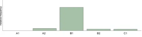
If we look at the data, we can see that mapping dis-tributions to labels is not straightforward, e.g. fig-ures 1 and 2 show the distributions of the wordsheta

(verb) ‘to be called’ andg¨ora(verb) ‘to do’. Using thesignificant onset of usealgorithm, we would pre-dict B1 as label for these words.

Figure 1:Frequency distribution of the wordheta‘to be called’

Figure 2:Frequency distribution of the wordg¨ora‘to do’

The verbsg¨oraandhetaare encountered very of-ten at the beginner level as beginners learn to intro-duce themselves (e.g. Jag heter Peter. ‘My name is Peter.’) and talk about things they do.

Thus, common sense dictates that we cannot sim-ply use frequency distributions as indicators of when learners should be assumed to be able to start using certain words productively.

5.3 Word diversity

In contrast to directly mapping frequency distribu-tions to labels, we have found that normalizing the frequencies using word diversity improved results significantly. We calculate word diversity for each word by looking at how often the word was used at each level and how manydifferentlearners used the word at each level. Word diversity of a word wat levelLis calculated by dividing the number of oc-currences of the word at level Lby the number of distinct learnersdthat used the word at that level as shown in equation 2. The intuition is that if a word is used often at a certain level, but only by one learner, it is less representative of this level than if it is used by many different learners.

diversity(w, L) = count(w, L)

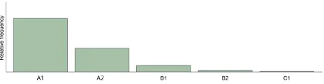
count(d, w, L) (2)

After normalizing the original frequency distribu-tion to fit into the interval 0-1, we average the word diversity distribution and the normalized frequency distribution to arrive at a new distribution. Figure 3 shows the new distribution forheta.

Figure 3:New distribution of the wordheta‘to be called’

We can see that including word diversity shifts the original frequency distribution towards the left, with a peak at A1. Incidentally, the automatically predicted level for this word is also A1; however, it should be noted that the calculation of the significant onset of use differs from simply taking the peak. For example, figure 4 shows the recalculated distribution for the relatively common verbg¨ora‘to do’. We can

see maxima at A2 and B2, but the algorithm predicts the more plausible A1.

Figure 4:New distribution of the wordg¨ora‘to do’

6 Distributional semantics

We used the gensim implementation of Word2Vec (Mikolov and Dean, 2013) to create a vector space model of our corpus of essays. Since we don’t have a gold standard to validate our results, we wanted to see to what extent we might reproduce the same es-say level labeling through a different method. We have 339 essays, each one labeled with a CEFR grade as assigned by a teacher. Given this data, we built two different kinds of semantic spaces: a sim-ple context-based space taking into account a num-ber of words at the left and right of the given lemma; and an “indexed” approach which, for each word in an essay, takes into account both its context and the proficiency level of the whole essay. In other terms, the proficiency level of an essay is treated as contex-tual information to build a word’s distributional vec-tor, in the same way as other words. We also tried a stricter approach where we constrained the system to take into consideration only the proficiency level to build the distributional vector of a lemma, under the assumption that words sharing the same proficiency-related distributional profile would tendentially clus-ter together in a semantic space, without need for further information.

It is important to understand what kind of spaces these approaches create. If we don’t take proficiency levels directly into account, we generate a traditional semantic space where words that have similar texts cluster together. The problem in creating con-sistent proficiency-related vocabularies with this ap-proach is clear: if a C1 word happens to be a syn-onym of an A1 word (and thus used in similar con-texts) it will be more similar to such A1 word than to other C1 words.

them-selves “points” in the multidimensional semantic space: thus, words that occur in the same level will tend to be near, but also a word will be nearer to the proficiency label it shares most context with. The advantage of this method is that we can directly compute the similarity between a lemma and a pro-ficiency level; the disadvantage is that contextual information could actually work as noise. For ex-ample, if a complex word asangel¨agenheter ‘con-cerns’ (noun) co-occurs with a simple word as tis-dag ‘Tuesday’, and tisdag mainly happens at level A1, thenangel¨agenheterand the point ‘A1’ will be-come closer.

If, finally, we only take into account the profi-ciency level, words that occur in the same level will be similar in the semantic space. In this case we cannot meaningfully compute a word-level similar-ity but the risks of contextual noise are reduced. It can be interesting to note that since we are using a continuous semantic space we can try to predict the proficiency level (in a direct or indirect way) of full documents by averaging the individual vectors of their words.

We can use one of these models to compute the di-rect cosine similarity between a word and a level and that we could use to check whether the most sim-ilar words to a given level, e.g. B1, are the same we labeled as B1 in our frequency-based approach. On the other hand we can use the other model to see whether words cluster together consistently with our frequency-based lists.

7 Evaluation

The first reason we used a semantic space to model L2 essays vocabulary is to see whether, using a different approach, we might obtain results con-sistent with the frequency-based learner-augmented lists we described in the first part of the paper. As we explained, we don’t expect simple distributional models to work very well on this task, but we tried to monitor the performance of a so-called “indexed method” to try to make words characteristic of spe-cific proficiency level closer between them and to the level label itself in the semantic space. If a se-mantic space model trained as described above re-produces the predictions of our frequency-based lists (for example clustering together words that are in the

same proficiency level in the lists) we could be a lit-tle more confident that our labeling is sensible. To test this we randomly selected 100 words from our frequency lists, equally distributed among the 5 pro-ficiency classes A1-C1. On these 100 words we ran two tests: one based on the word-label cosine simi-larity, and one based on the word-word cosine sim-ilarity. The first test selects, in the semantic space, the nearest proficiency label to a given word. For ex-ample given the wordeftersom‘because’, we select the label holding the nearest cosine similarity with it, for example “A2”; ifeftersom is mapped to the level A2 according to our mapping algorithm, we have an agreement among our models. We can then count how many “nearest labels” coincided with the frequency-based prediction and determine to what extent the two approaches are consistent in model-ing the data.

The second test consists in simply retrieving, for every word, itsn-nearest neighbours in the semantic space. We can then determine whether these neigh-bours belong to the same proficiency level of the given word in the frequency list. For example, we can retrieve the nearest neighbours of the word tis-dag ‘Tuesday’ and find them to be l¨ordag ‘Satur-day’ andtr¨ott ‘tired’. If these two words are of the same proficiency level astisdagin our lists, we can suppose a certain consistency between the two ap-proaches.

Table 3 shows the results for the different tests and different models. We tested two indexed models, with window size 1 and 60 respectively, and a non-indexed model with window size 10. The numbers indicate how many items were assigned the same proficiency levels in both the semantic space model and the frequency-based mapping, with the upper limit being 100. We are indicating counts, but as the upper limit is 100, the numbers can also be un-derstood as percentages. For the word-word similar-ity test, we look at the first, second and third most similar words according to the cosine similarity and check whether their proficiency label is the same as the one assigned by the frequency-based mapping. The figures in parentheses indicate the number of

close mismatches(off-by-one errors).

word-label test word-word similarity test (n-nearest neighbours) 1st nearest 2nd nearest 3rd nearest

Indexed model (w=1) 33 (29) 35 (36) 27 (46) 34 (37)

Indexed model (w=60) 51(13) 67(31) 44(37) 46(37) Non-indexed model (w=10) 18 (31) 38 (38) 24 (49) 28 (34)

Table 3:Results

over five proficiency levels, accuracies of 51% and 67% are encouraging numbers. What is maybe even more interesting is the number ofclose mismatches. These cases are interesting because they could show that the models are setting different boundaries, but tendentially agree on the general progression of the vocabulary. If the number of close mismatches is high, it means that we have many cases where A1 words (in our frequency list) are “labeled” as, or cluster with, A2 words in the semantic space: it is easy to see that similar cases are qualitatively very different from cases where an A1 word clusters with C1 vocabulary. The large presence of similar cases in our results brings us the next reason that induced us to use semantic spaces: they can give nuanced results. If we use a distributional space to label a lemma, we’ll have not only the most probable level of such lemma, but also its distance to the next and previous level. For example, both our frequency list and our best performing semantic space label resa

‘to travel’ as an A2 word. From the semantic space, we can also see that it is much closer to B1 than to A1 – we can suppose that it is a rather “advanced” word that tends to lie between A2 and B1. In the same way,fredag‘Friday’, labeled as A2 by the fre-quency lists, clusters in our space both with A2 and (less closely) A1 lemmas, showing that it is likely to be a term on the “easy” spectrum of the A2 vocabu-lary.

8 Lexical complexity analysis

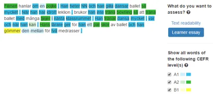
In order to analyze an unseen learner essay, we anno-tate the essay using the Sparv pipeline (Borin et al., 2012). This step results in a lemmatized and part-of-speech tagged text. Each lemma is then looked up in the previously calculated word list and marked as being of the level indicated in the word list.

We can then simply visualize this information us-ing a graphical user interface1 as shown in figure 5. After entering a text in the text box, it is possible to highlight words of certain CEFR levels. This kind of visualization can give a good impression of the distribution of word levels in a text.

Figure 5:Text evaluation: Visualization

We can also use the word list to predict the over-all proficiency level of the essay. Rather than being used on its own, it is incorporated into larger sys-tems. Recent research has shown that substituting traditional frequency based lists by distributionally mapped word lists in machine learning based auto-matic essay grading systems results in significantly better predictions (Pil´an et al., 2016).

9 Conclusion

In this paper we have shown how lists of frequency distributions of lexical items over CEFR levels can be used for lexical complexity analysis by linking each word to a single CEFR label. We have found that augmenting frequency based lists with learner counts yields more plausible mappings than taking into account only the frequency information. Using a semantic space approach we have shown that our results are consistent across different models. Fi-nally, we have shown how this information can be visualized and used for essay grade prediction.

1

References

R. Artstein and M. Poesio. 2008. Inter-coder agreement for computational linguistics. Computational Linguis-tics, 34(4):555–596.

Lars Borin, Markus Forsberg, and Johan Roxendal. 2012. Korp - the corpus infrastructure of Spr˚akbanken. In

LREC, pages 474–478.

Council of Europe. 2001. Common European Frame-work of Reference for Languages: Learning, Teach-ing, Assessment. Press Syndicate of the University of Cambridge.

Eva Forsbom. 2006. A swedish base vocabulary pool.

InSwedish Language Technology conference,

Gothen-burg.

Thomas Franc¸ois, Elena Volodina, Ildik´o Pil´an, and Ana¨ıs Tack. 2016. SVALex: a CEFR-graded Lexical Resource for Swedish Foreign and Second Language Learners. InLREC 2016.

H˚akan Jansson, Sofie Johansson Kokkinakis, Judy Ribeck, and Emma Sk¨oldberg. 2012. A Swedish Aca-demic Word List: Methods and Data. InProceedings

of the 15th EURALEX International Congress, pages

7–11.

Adam Kilgarriff, Frieda Charalabopoulou, Maria Gavrili-dou, Janne Bondi Johannessen, Saussan Khalil, Sofie Johansson Kokkinakis, Robert Lew, Serge Sharoff, Ravikiran Vadlapudi, and Elena Volodina. 2014. Corpus-based vocabulary lists for language learners for nine languages. Language resources and evaluation, 48(1):121–163.

K. Krippendorff. 1980. Content Analysis: An

Introduc-tion to Its Methodology. Chapter 12. Sage, Beverly

Hills, CA.

Lorena Llozhi. 2016. SweLL list. A list of productive vocabulary generated from second language learners’ essays. Master’s Thesis. University of Gothenburg. Tomas Mikolov and Jeff Dean. 2013. Distributed

rep-resentations of words and phrases and their composi-tionality. Advances in neural information processing systems.

Katarina Heimann M¨uhlenbock and Sofie Johansson Kokkinakis. 2012. SweVoc-a Swedish vocabulary re-source for CALL. In Proceedings of the SLTC 2012 workshop on NLP for CALL; Lund; 25th October; 2012, number 080, pages 28–34. Link¨oping University Electronic Press.

Ildik´o Pil´an, David Alfter, and Elena Volodina. 2016. Coursebook texts as a helping hand for classifying lin-guistic complexity in language learners’ writings. In

Proceedings of the workshop on Computational

Lin-guistics for Linguistic Complexity (CL4LC). COLING

2016. Osaka, Japan.

Elena Volodina, Ildik´o Pil´an, Stian Rødven Eide, and Hannes Heidarsson. 2014. You get what you anno-tate: a pedagogically annotated corpus of coursebooks for Swedish as a Second Language. In Proceedings of the third workshop on NLP for computer-assisted

language learning at SLTC 2014, Uppsala University,

number 107. Link¨oping University Electronic Press. Elena Volodina, Ildik´o Pil´an, and David Alfter. 2016a.

Classification of Swedish learner essays by CEFR lev-els. InProceedings of EuroCALL 2016.