A Method for Experimental Events that Break Cointegration: Counterfactual Simulation

A Method for Experimental Events that

Break Cointegration: Counterfactual

Simulation

Bell, Peter N

University of Victoria

7 February 2014

Online at

https://mpra.ub.uni-muenchen.de/53523/

A Method for Experimental Events that Break

Cointegration: Counterfactual Simulation

Peter Bell

University of Victoria

A Method for Experimental Events that Break Cointegration:

Counterfactual Simulation

Peter Bell

Abstract: In this paper I develop a method to estimate the effect of

an event on a time series variable. The event is framed in a

quasi-experimental setting with time series observations on a treatment variable,

which is affected by the event, and a control variable, which is not. Prior to

the event, the two variables are cointegrated. After the event, they are not.

Since the event only affects the treatment variable, the method uses

observations on the control variable after the event and the distribution of

difference in differences before the event to simulate values for the

treatment variable as-if the event did not occur; hence the name

counterfactual simulation. I describe theoretical properties of the method

and show the method in action with purpose-built data.

Keywords: Quasi-experiment, cointegration, time series,

counterfactual, simulation

1. Introduction

In this paper I develop a method to estimate the effect of an event on a time series variable.

I describe the method in terms of a quasi-experiment, with observations on treatment and control

variables, before and after the event occurs. There are many situations in economics where this

method may be helpful, from comparing stock prices to unemployment levels between countries.

I intend to apply the method to farmland ownership restrictions in Saskatchewan as part of my

I refer to my method as Counterfactual Simulation because it produces a distribution for

the treatment variable as-if the event never occurred. However, I recognize that this term was

used before in an influential paper by Christian Upper at the Bank for International Settlements

(2007). It is fair to re-use the term here because our methods and topics are different, but I

recognize the initial contribution by Dr. Upper. Writing at the beginning of the global financial

crisis in August 2007, Upper focuses on risks of contagion within interbank markets. With

remarkable prescience he notes that researchers have little data for events of interest because

important banks are often bailed-out (2007, p. 9). He provides a way forward: “Counterfactual simulations, by contrast, allow researchers to more or less freely specify the scenario they are

interested in, without regard to whether similar events have happened in the past” (2007, p. 3). Although this may seem like an obvious type of risk management activity, it is a sophisticated

process that requires a large number of assumptions, which allow for criticisms that the results

do not have a “gentlemanly distance” from the assumptions (2007, p. 18). I hope that such criticism does not impede the value that Upper’s methods can offer to studies of systemic risk.

My Counterfactual Simulation (CS) method uses an experimental design with observations

on treatment and control groups, before and after an intervention. This design is a classical

concept in the applied econometrics literature, as described in the popular textbook by Joshua

Angrist and Jörn-Steffen Pischke (2009). In particular, Angrist and Pischke use this design to

introduce difference-in-differences (diff-diff) models. The basic diff-diff setting compares the

effect of an intervention across two dimensions (treatment/control, before/after event) but it can

be generalized to include an arbitrary number of dimensions (p. 241). My CS method adds a

third dimension (time), which opens the discussion to time series econometrics.

Cointegration is a classic method from time series econometrics pioneered by Robert Engle

& Clive Granger (1987) for situations where multiple variables share similar growth rates. For

the cases I consider here, cointegration means that the diff-diff is stationary (no unit root in U(t)). The reader may notice an immediate connection between cointegration and quasi-experiments,

which is reflected in the substantial literature on structural breaks in cointegration; for example,

the textbook on Unit Roots, Cointegration, and Structural Change (Maddala & Kin, 1998). Such attention is well deserved because a structural break can confound estimation. Allen Gregory

and Bruce Hansen (1996) propose a test for structural breaks in cointegration and use it to find

discussion shows that cointegration can provide an important set of tools to model economic

variables that have dynamic statistical relationships.

My paper focuses on events that break cointegration. As I showed above, there is research

on events that move variables from one cointegration relationship to another, but it is more

difficult to gain analytic traction when the model leaves behind the stationary assumptions. New

thinking is starting to improve the situation. In particular, Ole Peters develops a new solution to

the ancient St. Petersburg paradox. Peters’ new solution resolves a problematic assumption in a cornerstone of modern economic theory by giving careful consideration to time averages versus

ensemble averages, which are different in non-stationary or non-ergodic settings (2011a, 2011b).

In this paper I use ensemble averages to make draws from the distribution of the diff-diff and

simulate data for the treatment variable. I intend to use time averages in future research.

The CS method uses simulation to develop economic insight. I do not make inference

from coefficients in a regression model; rather, I calculate distributions for variables of interest

directly and compare the simulated distributions with observed values. This focus on

simulation-based methods is related to a controversial debate in economics around the methodological risks

of strict statistical methods and imprecise distinctions between statistical significance and

economic significance (McCloskey & Ziliak, 1996).

In this paper I introduce the CS method in a theoretical framework and provide an example

of the method in action with purpose-built data. In Section 2 I introduce the CS method and

describe some basic properties with algebraic and numerical analysis. In Section 3 I build a

dataset where the CS method applies and show how to use the method to estimate the effect of an

event using an asymptotically large number of paths. I provide an appendix which contains

Matlab code to replicate all of the numerical results used in the paper.

2. Model for Data with and without Cointegration

The basic cointegration model has observations on two time series variables, X(t) and Y(t). I construct U(t) as the difference between them in Equation (1) and 𝑑𝑈

𝑑𝑡 as the diff-diff in Equation

(1) 𝑋(𝑡) − 𝑌(𝑡) = 𝑈(𝑡)

(2) 𝑑𝑈

𝑑𝑡 = 𝑑𝑋

𝑑𝑡− 𝑑𝑌 𝑑𝑡

To set the stage for my CS method, I specify the data generating process for X(t) and Y(t)

in terms of first-differences. Throughout, X(t) represents the control variable and Y(t) represents the treatment variable. I assume each variable has an individual noise term that is independent

and identically distributed over time (𝜀𝑋, 𝜀𝑌~𝑖𝑖𝑑).

Before the event, I assume that both X(t) and Y(t) have a slow moving, trend growth rate that I denote 𝛼. Think of 𝛼 as a random variable with significant autocorrelation. Since 𝛼 is the

trend growth rate for both X(t) and Y(t), as shown in Equations (3) and (4), the trends cancel in the diff-diff, Equation (5). It follows that the diff-diff is stationary.

(3) 𝑑𝑋

𝑑𝑡 = 𝛼 + 𝜀𝑋

(4) 𝑑𝑌

𝑑𝑡 = 𝛼 + 𝜀𝑌

(5) 𝑑𝑈

𝑑𝑡 = 𝜀𝑋− 𝜀𝑌

After the event I assume the treatment variable follows a different trend, which I denote 𝛽

in Equation (6). The control variable is still described by Equation (3). The trend growth rates

(𝛼, 𝛽) do not cancel in the diff after the event, as in Equation (7), and it follows that the

diff-diff is non-stationary (U(t) has a unit root). I provide an example of data with such properties in Section 3.

(6) 𝑑𝑌

𝑑𝑡 = 𝛽 + 𝜀𝑌

(7) 𝑑𝑈

𝑑𝑡 = 𝛼 − 𝛽 + 𝜀𝑋− 𝜀𝑌

To describe my CS method, I introduce three new variables. The first variable is the

change for the treatment variable at a certain time after the event as-if the event did not occur

(𝑑𝑌

𝑑𝑡(𝑡)

̃_{), which is the counterfactual variable. The second variable is an observation on the}

control variable for a specific time after the event (𝑑𝑋

𝑑𝑡(𝑡)), which is the benchmark for the

simulation. The first and second variables are associated with the same point in time. The third

variable is a draw from the distribution of the diff-diff before the event (𝑑𝑈

𝑑𝑡

̃_{), which is stationary.}

I combine the second and third variable to get a hypothetical value for the treatment variable at a

(8) 𝑑𝑌

𝑑𝑡̃ =(𝑡) 𝑑𝑋

𝑑𝑡(𝑡) − 𝑑𝑈

𝑑𝑡

̃

To establish properties of the counterfactual variable (𝑑𝑌

𝑑𝑡̃(𝑡)), I replace the two terms on

the right hand side of Equation (8) with their definitions. The observation for the control

variable (𝑑𝑋

𝑑𝑡) is based on Equation (3) and the draw from the diff-diff ( 𝑑𝑈

𝑑𝑡

̃_{) is based on Equation}

(5). Together, this produces Equation (9).

(9) 𝑑𝑌

𝑑𝑡̃ = 𝛼 + 𝜀(𝑡) 𝑋− 𝜀𝑋̃+ 𝜀𝑌

To move one step further, I recall the assumption that the noise terms are independent.

Independence means that random draw of the sum of variables is equal to a sum of two random

draws (𝜀𝑋̃ = 𝜀+ 𝜀𝑌 ̃ + 𝜀𝑋 ̃𝑌). This insight yields Equation (10), which reveals important properties of the counterfactual variable and the CS method.

(10) 𝑑𝑌

𝑑𝑡̃ = (𝛼 + 𝜀(𝑡) ̃) + (𝜀𝑌 𝑋− 𝜀̃)𝑋

In Equation (10), the first term (𝛼 + 𝜀̃)𝑌 behaves like the true variable (𝑑𝑌

𝑑𝑡(𝑡)) from

Equation (4). However, the second term (𝜀𝑋− 𝜀̃𝑋) has different behaviour that I describe as

estimation error. This estimation error has zero mean because the terms are drawn from the same distribution (𝜀𝑋, 𝜀̃~𝑖𝑖𝑑𝑋 ) but is not equal to zero because the variables represent two different draws from the same distribution. The estimation error has variance that is twice as

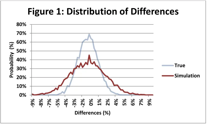
Figure 1 shows that the counterfactual variable does indeed have larger variance than the

true variable. To calculate this result I assume the noise terms have a normal distribution with

standard deviation 1.5% (𝜀𝑋, 𝜀𝑌~𝑖𝑖𝑑 𝑁(0,0.015)). The soft-blue “True” line represents the model in Equation (4), differences for the treatment variable before the event. The dark-red

“Simulation” line represents the distribution of the counterfactual variable ( 𝑑𝑌

dt̃(𝑡)) from

Equation (8).

(11) 𝑌(𝑇)̃ = 𝑌(𝑆) ∏ [1 +𝑑𝑌

𝑑𝑡̃ ](𝑡) 𝑇

𝑡=𝑆+1

So far I have only described the counterfactual variable in terms of differences. However,

the CS method provides a way to calculate the levels for the counterfactual variable. Equation

(11) describes how to use the method to simulate the level of the counterfactual variable. In

Equation (11), time t=S denotes the time when the event occurs, time t=T denotes the time that we want to simulate the counterfactual for (T>S). I calculate the level at time T by compounding the differences of the counterfactual differences from time S+1 to T, which is a standard

calculation for compounding growth rates. Equation (11) shows that the CS method creates an

entire distribution for the levels of the treatment variable at a certain time as-if the event did not

occur (𝑌(𝑇)̃).

Based on Figure 1, I expect that the simulated levels will have different properties from the

true levels for the treatment variable. I explore this using simulation in Figure 2.

0% 10% 20% 30% 40% 50% 60% 70% 80%

-9% -8% -7% -5% -4% -3% -2% 0% 1% 2% 4% 5% 6% 7% 9%

Pr

o

b

ab

il

ity

(

%

)

Differences (%)

Figure 1: Distribution of Differences

True

Figure 2 shows the distribution for the level of the treatment variable under simulation.

The diagram shows the distributions for a specific point in time (t=100), which may vary over time if the levels are non-stationary. Again, “True” refers to the treatment variable under Equation (4) and “Simulation” refers to data generated by the CS method (𝑌(100)̃ ). Notice that the two distributions have very similar centers, but the distribution from my CS method clearly

has larger variance. This suggests the estimation error identified in Equation (10) accumulates in

the differences and appears in the levels, as in Equation (11). Together, Figures 1 and 2 show

that data produced by the CS method has two sources of noise – the true noise in the data

generating process and additional noise (estimation error) introduced through the construction of

the counterfactual.

3. Simulation Example

I briefly describe the data generating process in simple terms. Before the event, I assume

that growth rates for both the treatment and control variables have a flat trend. After the event,

the treatment series (Y(t)) begins to follow a new trend with more frequent and larger decreases. This resembles a situation where two economic variables are similar at first, then an event

adversely affects one variable and causes it to deteriorate over time. I assume that I know all the

0% 2% 4% 6% 8% 10% 12% 14%

40 55 70 85 ₁₀0 ₁₁5 ₁₃0 ₁₄5 0_{16 17}5 ₁₉0 ₂₀5 ₂₂0 ₂₃5 ₂₅0

Pr

o

b

ab

il

ity

(%

)

Levels ($)

Figure 2: Distribution of Levels

True

relevant distributions for this demonstration but, in empirical applications, researchers will have

to contend with uncertainty about their estimates.

I construct data for the period before the event based on Equation (3) and (4) as follows. I

assume that 𝜀𝑋, 𝜀𝑌~𝑖𝑖𝑑 𝑁(0, 0.015). To build trend growth rates (𝛼) with autocorrelation, I use a moving average. Denote 𝑎(𝑖)~𝑖𝑖𝑑 𝑈(−0.05, 0.05) and 𝑘 = 10, then I define 𝛼(𝑡) by

Equation (12).

(12) 𝛼(𝑡) = ∑ 𝑎(𝑖)

𝑘 𝑡

𝑖=𝑡−𝑘

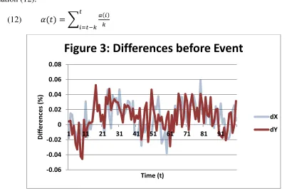
Figure 3 shows one round of data generated by my model for variables before the event.

Visual inspection suggests the two variables have similar growth rates, but do they pass a

statistical test for cointegration? I use the Dickey-Fuller test in Equation (13) to check this. The

null hypothesis for the test is is that the slope coefficient (b) is zero, which implies that the diff-diff are stationary (no unit root in U(t)) and the X, Y data are cointegrated. The alternative is that the slope is non-zero, the diff-diff are non-stationary and the data are not cointegrated.

(13) 𝑑𝑈

𝑑𝑡(𝑡) = 𝑎 + 𝑏 𝑑𝑈

𝑑𝑡(𝑡 − 1) + 𝑒(𝑡)

I find that, yes, the data in Figure 3 are cointegrated. The estimation results presented in

Table 1 show that the slope coefficient (b) is not different from zero at a 95% confidence level. My data generating process is working as intended for the period before the event.

-0.06 -0.04 -0.02 0 0.02 0.04 0.06 0.08

1 11 21 31 41 51 61 71 81 91

D

iff

e

re

n

ce

s

(%

)

Time (t)

Figure 3: Differences before Event

dX

Table 1: Cointegration Test with Data Before Event

Coefficient Estimate 95% Lower Bound 95% Upper Bound

Intercept (a) -0.001 -0.005 0.003

Slope (b) 0.027 -0.175 0.229

To create data without cointegration, I introduce a new trend for the treatment variable (𝑑𝑌

𝑑𝑡).

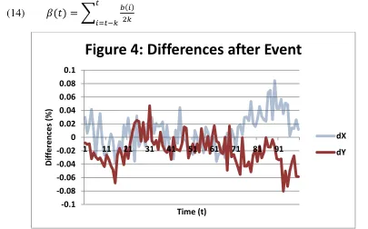
This new trend has higher probabilities of larger decreases, which can be seen in Figure 4: the

treatment variable has repeated decreases larger than 5% around time 90, which is different from

the behaviour of the treatment variable in Figure 3. The control variable (𝑑𝑋

𝑑𝑡) follows the same

trend as before, Equation (12). I denote the new trend as 𝛽 and construct it as a different path

from the same family of 𝛼. Let 𝑏(𝑖)~𝑖𝑖𝑑 𝑈(−0.05,0.05), then 𝛽(𝑡) is defined by Equation (14).

(14) 𝛽(𝑡) = ∑ 𝑏(𝑖)

2𝑘 𝑡

𝑖=𝑡−𝑘

Figure 4 shows one round of data for the variables after the event. The data is clearly

different from Figure 3 at some time intervals, such as times 70—90, but it is not clear if the differences are sufficient to register as not-cointegrated within the Engle-Granger framework.

Therefore, I use the Dickey-Fuller test to determine if the diff-diff in Figure 4 are stationary.

Table 2 shows that the data in Figure 4 is, indeed, not cointegrated. Technically, the diff-diff has

significant (positive) autocorrelation, which means it is not-stationary. This provides evidence

that my data generating process is working as intended for the period after the event.

-0.1 -0.08 -0.06 -0.04 -0.02 0 0.02 0.04 0.06 0.08 0.1

1 11 21 31 41 51 61 71 81 91

D

iff

e

re

n

ce

s

(%

)

Time (t)

Figure 4: Differences after Event

dX

Table 2: Cointegration Test with Data After Event

Coefficient Estimate 95% Lower Bound 95% Upper Bound

Intercept (a) 0.014 0.006 0.022

Slope (b) 0.523 0.350 0.696

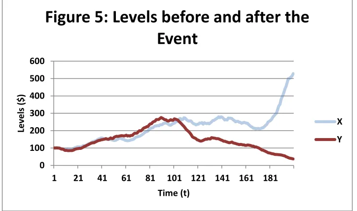
Figure 5 shows the levels for X(t) and Y(t) based on the differences shown in Figures 3 and 4. The Figure shows the entire simulation, which is 200 time steps long. The event occurs at

time 100. Notice how X(t) and Y(t) start to diverge after time 100 – this is because Y(t) is following a new trend with downward-bias.

Figure 6 shows an example of the CS method in action. The Figure zooms in on the

second half of Figure 5, after the event occurs. The dotted line (Y-Hat) is one version of the counterfactual variable from Equation (11). Notice how the dotted line tracks closely around the

control variable (X(t)), this occurs because the dotted line is built from the trend growth (𝛼) in the control group (X(t)). The simulated data (Y-Hat)has very different behaviour than the

observed data (Y-Observed), which illustrates the type of results that my CS method can produce. However, Figure 6 only shows a single path from the CS method. The method can

produce arbitrarily many paths. In fact, the method can produce an entire distribution for the

treatment variable ((𝑌(100)̃ ). I simulate 10,000 paths to estimate the distribution at each time

step. There are several ways to use this distribution to estimate the effect of the event ( event-effect). One way to measure the event-effect is to compare the observed level (Y(T)) and the

0 100 200 300 400 500 600

1 21 41 61 81 101 121 141 161 181

Level

s

($)

Time (t)

Figure 5: Levels before and after the

Event

X

median simulated value (𝑌(𝑇)̅̅̅̅̅̅), which is appropriate because it is robust to outliers. I denote this

measure for event-effect as E(T) and define it in Equation (15). (15) 𝐸(𝑇) = 𝑌(𝑇) − 𝑌(𝑇)̅̅̅̅̅̅

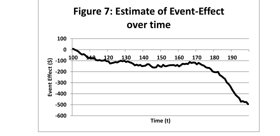
Since the measure of event-effect (E(T)) depends on time, the CS method provides a way to explore how the event-effect varies over time. Figure 7 shows the event-effect (E(T)) over the entire period after the event (100<T<200) using my simulations. Notice how the event-effect takes large negative values around time 190, which is the same time that the control variable

(X(t)) increases and the treatment decreases (Y(t)). This is the precisely the type of behaviour that the CS method is designed to capture.

0 100 200 300 400 500 600 700

100 110 120 130 140 150 160 170 180 190

Level

s

($)

Time (t)

Figure 6: Example of Single Path from

Method

X

Y-Observed

Y-Hat

-600 -500 -400 -300 -200 -100 0 100

100 110 120 130 140 150 160 170 180 190

E

v

e

n

t

E

ff

e

ct

($)

Time (t)

Figure 7 provides evidence to address the original research question: how has the event

affected the treatment variable over time and where would the treatment variable be if the event

never occurred?

4. Conclusion

In this paper I develop a method for quasi-experiments where an event breaks cointegration.

This is not just a structural change within a cointegration relationship; rather, it can deal with

situations where there is no cointegration after the event. The method extends the distribution of

the diff-diff before the event to the period after the event to simulate values for the treatment

variable as-if the event never occurred, hence the name Counterfactual Simulation (CS). I

explore properties of the CS method using analytic and numerical analysis. I show that the

counterfactual variable has two sources of noise: noise from the true data generating process, and

noise from estimation error. I argue that the simulated variable will have larger variance based

on theoretical grounds and show that this is true in simulation.

I also demonstrate how to use the method with purpose-built data. I simulate a time series

with length 100 both before and after the event, and show that the diff-diff are indeed stationary

before but not after. I show a single path for the counterfactual variable and discuss how to use

the distribution of the counterfactual variable to estimate the effect of the event over time. I

present a measure for the event-effect and show that it has intuitive behaviour in simulation.

This paper provides a foundation for the CS method that can be enhanced in several ways.

For example, it is possible to model uncertainty around the estimates of the distribution of the

diff-diff before the event or develop a formal testing procedure to determine if an event is

significant and conduct power analysis for the test. Both of these endeavours would be valuable

precursors to empirical applications of the method, of which there are many in our data-rich

world. The method raises other questions for me, such as the need for certain assumptions in the

classic model of cointegration (does each variable have to be individually stationary?) or the

References

Angrist, J.D. & Pischk, J.S. (2009). Mostly Harmless Econometrics. Princeton, NJ: Princeton University Press.

Bell, P. (2014). Farmland Ownership Restrictions: Between a Rock and a Hard Place.

Unpublished manuscript. University of Victoria, Canada. Retrieved from

http://mpra.ub.uni-muenchen.de/53033/

Engle, R.F. & Granger, C.W.J. (1987). Cointegration and error correction: Representation,

estimation, and testing. Econometrica, 55, 251—276.

Gregory, A.W. & Hansen, B.E. (1996). Residual-based tests for cointegration in models with

regime shifts. Journal of Econometrics, 70(1), 99—126.

Maddala, G.S. & Kin, In-Moo (1998). Unit Roots, Cointegration, and Structural Change. Cambridge, UK: Cambridge University Press.

McCloskey, D., Ziliak S.T. (1996). The Standard Error of Regressions. Journal of Economic Literature, 34, 97–114.

Peters, O. (2011a). The time resolution of the St. Petersburg paradox. Philosophical Transactions of the Royal Society A, 369(1956). 4913-4931.

Peters, O. (2011b). Menger 1934 Revisited. Unpublished manuscript, Imperial College London. Retrieved from http://arxiv.org/abs/1110.1578

Upper, C. (2007). Using Counterfactual simulations to assess the danger of contagion in

interbank markets. BIS Working Paper No. 234. Retrieved from

Code Appendix:

Counterfactual Simulation

Peter Bell

University of Victoria

% Code has three sections. Code written for Matlab 2010. %

%

%% Section 1: Simulate a single path to show breakpoint in cointegration.

% Set random seed to allow replication of results.

s = RandStream('mcg16807','Seed',0) RandStream.setDefaultStream(s)

% Set length of path and trend growth rates.

% Note: a~U(-0.1,0.1) and b~U(-0.12,0.08) to reflect beta is down-trend.

n1 = 100; n2 = 100; k = 10;

a = (randi(20,[n1+n2+k,1])-10)/100; b = (randi(20,[n1+n2+k,1])-12)/100;

for i = 1:n1+n2

alpha(i) = mean(a(i:i+k)); beta(i) = mean(b(i:i+k));

end

% The idiosyncratic noise terms are iid, N(0,0.015).

sigmaX=0.015; sigmaY=0.015; epsX=sigmaX*randn(n1+n2,1); epsY=sigmaY*randn(n1+n2,1);

% The differences before the event (dX0) have the same trend.

dX0 = alpha(1:n1)' + epsX(1:n1); dY0 = alpha(1:n1)' + epsY(1:n1); dU0 = dX0 - dY0;

% The differences after the event (dX1) have different trends.

dX1 = alpha(n1+1:n1+n2)' + epsX(n1+1:n1+n2); dY1 = beta(n1+1:n1+n2)' + epsY(n1+1:n1+n2); dU1 = dX1 - dY1;

% I preform regression on the diff-diff before and after the event.

dU0Lag = lagmatrix(dU0,1);

regB0 = [ones(n1-1,1), dU0Lag(2:n1)]; [b0,bInt0] = regress(dU0(2:n1), regB0); dU1Lag = lagmatrix(dU1,1);

regB1 = [ones(n1-1,1), dU1Lag(2:n1)]; [b1,bInt1] = regress(dU1(2:n1), regB1);

% I build the levels of the variables to show affects of the event.

X(1)=100; Y(1)=100;

dX = [dX0; dX1]; dY = [dY0; dY1]

for i = 2:n1+n2

Y(i) = Y(i-1)*(1+dY(i-1)) X(i) = X(i-1)*(1+dX(i-1))

end

% To collect key data variables together.

coint1 = [b1,bInt1];

%% Section 2: demonstrate method. %

% First I simulate a single path with the CS method.

% I build the diff-diff as-if I know it's true distribution.

dUHat = sigmaX*randn(n2,1)-sigmaY*randn(n2,1);

% I build hypothetical changes based on observed control and diff-diff.

dYHat = dX(n1+1:n1+n2)+dUHat; YHat(1) = Y(n1)

for timeCount = 2:n2

YHat(timeCount) = YHat(timeCount-1)*(1+dYHat(timeCount-1));

end

% To collect key variables.

simPath = [X(n1+1:n1+n2)' Y(n1+1:n1+n2)' YHat']

% Second I show how to calculate policy-effect using the CS method.

numSim = 100;

for i = 1:numSim

dUHat = sigmaX*randn(n2,1)-sigmaY*randn(n2,1); dYHat = dX(n1+1:n1+n2)+dUHat;

YHat(1) = Y(n1); for timeCount = 2:n2

YHat(timeCount) = YHat(timeCount-1)*(1+dYHat(timeCount-1)); end

simLevel(i,1)=YHat(5);

end

% To collect key variables.

simResults = [ Y(n1+5) median(simLevel) mean(simLevel)]

% Third, I calculate levels-effect over time

for j = 1:100 numSim = 100; for i = 1:numSim

dUHat = sigmaX*randn(n2,1)-sigmaY*randn(n2,1); dYHat = dX(n1+1:n1+n2)+dUHat;

YHat(1) = Y(n1); for timeCount = 2:n2

YHat(timeCount) = YHat(timeCount-1)*(1+dYHat(timeCount-1)); end

simLevel(i,1)=YHat(j); end

simEffect(j,1) = Y(n1+j)-median(simLevel)

end

clear all

% As in Section 1.

s = RandStream('mcg16807','Seed',0) RandStream.setDefaultStream(s) n2 = 100; k = 10;

sigmaX = 0.015; sigmaY = 0.015;

% First simulation: differences. This is one step in each path, simualted % ten thousand times. Shows the difference of distribution of treatment % (dy) as if no event and as estimated using my method.

aPrime = (randi(20,[k,1])-10)/100; alphaPrime = mean(aPrime);

numSimDiff = 10000

for i =1:numSimDiff

epsX1=sigmaX*randn(1,1); epsX2=sigmaX*randn(1,1); epsY=sigmaY*randn(1,1);

dYObs = alphaPrime(1) + epsY; dYHat = dYObs + epsX1 - epsX2; simDiffs(i,1) = dYObs;

simDiffs(i,2) = dYHat;

end

% Second simulation, levels. Each path has 100 time steps and I simulate % ten thousand paths. The results shows the distribution for the Y

% variable as-if there was no event, and as-estimated using my method.

numSimDiff = 10000; nStep=100; k=10;

for simCount =1:numSimDiff

aPrime = (randi(20,[nStep+k,1])-10)/1000; for aCount = 1:nStep

alphaPrime(aCount) = mean(aPrime(aCount:aCount+k)); end

epsX1=sigmaX*randn(nStep,1); epsX2=sigmaX*randn(nStep,1); epsY=sigmaY*randn(nStep,1); dYObs = alphaPrime' + epsY; dYHat = dYObs + epsX1 - epsX2; YObs(1)=100; YHat(1)=100; for levelCount = 2:nStep

YObs(levelCount) = YObs(levelCount-1)*(1+dYObs(levelCount-1)); YHat(levelCount) = YHat(levelCount-1)*(1+dYHat(levelCount-1)); end

simLevels(simCount,1) = YObs(nStep); simLevels(simCount,2) = YHat(nStep);

end