Stress Testing and Modeling of Rating Migration under the Vasicek Model Framework Empirical approaches and technical implementation

Munich Personal RePEc Archive

Stress Testing and Modeling of Rating

Migration under the Vasicek Model

Framework - Empirical approaches and

technical implementation

Yang, Bill Huajian and Du, Zunwei

18 June 2015

Online at

https://mpra.ub.uni-muenchen.de/65168/

Stress Testing and Modeling of Rating Migration

under the Vasicek Model Framework



- Empirical approaches and technical implementation

(Pre-typeset version)

(Final version is published in "Journal of Risk Model Validation", Vol.9 / No.2, 2015)

Bill Huajian Yang Zunwei Du

Abstract

Under the Vasicek asymptotic single risk factor model, stress testing based on rating transition probability involves three components: the unconditional rating transition matrix, asset correlations, and stress testing factor models for systematic downgrade (including default) risk. Conditional transition probability for stress testing given systematic risk factors can be derived accordingly. In this paper, we extend Miu and Ozdemir’s work ([14]) on stress testing under this transition probability framework by assuming different asset correlation and different stress testing factormodel for each non-default rating. We propose two Vasicek models for each non-default rating, one with a single latent factor for rating level asset correlation, and another multifactor Vasicek model with a latent effect for systematic downgrade risk. Both models can be fitted effectively by using, for example, the SAS non-linear mixed procedure. Analytical formulas for conditional transition probabilities are derived. Modeling downgrade risk rather than default risk addresses the issue of low default counts for high quality ratings. As an illustration, we model the transition probabilities for a corporate portfolio. Portfolio default risk and credit loss under stress scenarios are derived accordingly. Results show, stress-testing models developed in this way demonstrate desired sensitivity to risk factors, which is generally expected.

Keywords: Stress testing, systematic risk, asset correlation, rating migration, Vasicek model, bootstrap aggregation

1. Introduction

Stress testing is important for financial institutions either for regulatory requirements or for internal capital allocation ([1], [3], [7], [18]). In practice, stress testing focuses on systematic risk, with shocks originating from the market or macroeconomic factors ([5], [7], [19]).

Let

{

R

_i

|

1



i



k

}

denote a rating system with k ratings, with lower indexes i indicating lower default risk. Thus

R

₁is the best quality rating and

R

kis the worst rating, i.e., the default rating.

For a credit portfolio, stress testing can be implemented through modeling the conditional transitional probabilities under systematic risk ([2], [14]). The transition probabilities for an entity with a non-default rating

R

iare assumed to be governed by a latent random variable

z

i, called the firm’s

normalized asset value, which splits into two parts as:

where

s

i represents the systematic risk (i.e., the common risk to all entities in the rating), while



i

represents the idiosyncratic risk. The constant



i is called the asset correlation. It is assumed that



Bill Huajian Yang, and Zunwei Du, Enterprise Stress Testing, Royal Bank of Canada

Mail address: 155 Wellington Street W 16th floor, Toronto, ON, Canada, M5V 3K7

The views expressed in this article are not necessarily those of Royal Bank of Canada or any of its affiliates. Please direct any comments to [email protected], phone: 416-313-1245

) 1 , 0 ( ~ ), 1 , 0 ( ~ , 1 0

,

1 s N N

s

there exist threshold values{bij}such that a firm’s rating migrates from

R

itoRj or worse (called

downgrade (including default) risk) when

z

ifalls below the threshold value bi(kj1).

Modeling for stress testing purposes for a credit portfolio under this framework involves: (a) Determining the threshold values{bij}(or equivalently, the unconditional transition

probabilities).

(b) Estimating the asset correlation



ifor each non-default rating.

(c) Modeling the downgrade risk by a multifactor model for each non-default rating. (d) Deriving conditional transition probabilities given scenario risk factors thus assessing

portfolio level credit loss.

While threshold values{bij}can be estimated by using historical point-in-time migration matrices (see

section 2), the estimation of asset correlations and modeling of conditional downgrade risk by factor models are more challenging. Miu and Ozdemir ([14]) propose approaches to deriving the conditional transition probabilities based on a factor model for the systematic risk s:

s  f(x₁,x₂,...,xm)e, e~ N(0,



e2) (1.2)

by assuming the same systematic risk and same asset correlation for all non-default ratings. Miu and Ozdemir also show how parameters of model (1.2) and those from (a)-(c), including threshold values

}

{bij , can be estimated simultaneously in one single process of likelihood maximization.

We extend Miu and Ozdemir’s work to a more granular rating level, by assuming different asset correlation



i and different systematic risk

s

i for each default rating. Specifically, for a

non-default rating

R

i, let

d

i

(

s

i

)

denote the downgrade probability given systematic risk

s

i. We proposed

two Vasicek models, each with a latent random effect, for stress testing purposes:

d

i

(

s

i

)





(

a

i₀



a

i₁

s

i

)

,

s

i

~

N

(

0

,

1

)

(1.3)

( ) ( ), ~ (0, 2( ))

2 1 1

0 i i s im m i i i

i i

i s a a x a x a x e e N e

d     



(1.4)

where



denotes the standard normal cumulative distribution, and

x

1

,

x

2

,

...,

x

mare scenario or

macro risk factors. As shown in later sections, asset correlation



i and conditional transition

probabilities can be derived accordingly from these two stress testing models, given the threshold values {bij} (see Lemma 3.1 and Theorem 3.3).

The advantages for the proposed approaches are the following:

(1) Asset correlations and stress testing factor models are differentiated between non-default ratings, achieving desired risk sensitivity for the stress testing models under stress scenarios. (2) Similar to the results by Miu and Ozdemir ([14]), analytical formulas for conditional transition

probabilities are derived.

(3) Parameters in (a)-(c) are estimated separately, expert judgements and adjustments for threshold values {bij}and asset correlations are made possible.

Models (1.3)-(1.4) can be fitted effectively by using, for example, SAS non-linear mixed procedure ([21]), assuming a binomial distribution for the event count given the event probability. We will propose a two-step fitting procedure in section 3.3 for training the model (1.4): first by a master model for all non-default ratings targeting the portfolio default risk, and then calibrating this master model to rating level for each non-default rating, targeting the downgrade risk.

The paper is organized as follows: We review in section 2 the Vasicek asymptotic single risk factor model (ASRF) for modeling of rating migration. In section 3, we propose the stress testing models (1.3)-(1.4), and derive the analytical formulas for conditional transition probabilities. Parameter estimation methodologies, including the bootstrap aggregation technique (called bagging, for addressing the time series serial correlation), are reviewed in section 4. In section 5, we validate the proposed approaches by building stress testing models for a US corporate portfolio. Portfolio credit loss and default risk on stress scenarios are assessed accordingly.

The author thanks Dr. Clovis Sukam for his critical reading of the manuscript.

2. Rating Migration under the Vasicek Asymptotic Single Risk Factor Model Framework 2.1. The Vasicek Asymptotic Single Risk Factor Model

Under the Vasicek asymptotic single risk factor model ([2], [9], [11], [12], [13], [14], [20]), default risk for an entity is driven by a latent variable z, the normalized asset value of the entity.Adefault event occurs in horizon if this normalized asset value falls below a threshold value,called default point. For a group of risk homogenous entities, z splits into two parts:

where s represents the systematic risk (i.e., the common risk), common to all entities in the group, while



represents the idiosyncratic risk. The constant



is called the asset correlation of the group.

2.2. The Unconditional Rating Migration Matrix

We assume that entities in the same rating are risk homogeneous. Thus model (2.1) applies. Given a non-default rating

R

i, we assume that there exist k threshold values

bi1 bi2 ...bi(k1) bik() (2.2)

such that an entity will migrate to ratingRjor worse in horizon if z falls below bi(kj1),

i.e.,zbi(kj1).

Denote bypij the unconditional transition probability of migrating from

R

i toRj, anddijthe

unconditional transition probability from

R

i toRjor worse. This means

p

ik

(



d

ik

)

is the

unconditional default probability for rating

R

i. The following propositions hold and can be found in

([2], [14]).

Proposition 2.1

. (a) If

j



1

,

dij 1

.

(b) If

j



1

,

dij P(zbi(kj1)(bi(kj1))

) 1 . 2 ( ) 1 , 0 ( ~ ), 1 , 0 ( ~ , 1 0

,

1 s N N

s

Proposition 2.2

(a)

p

ik



d

ik





(

b

i1

)

and

pi1 1(bi(k1))

(b) If

1



j



k

then

pij (bi(kj1))(bi(kj))dij di(j1)

.

Consequently, given the unconditional transition matrixT (pij), the threshold values{bij}in (2.2)

can be determined sequentially, first

b

i1 by Proposition 2.2 (a), then

b

i2 by Proposition 2.2 (b) and

Proposition 2.1 (b), and so on.

2.3. Calibration of the Unconditional Rating Migration Matrix

The unconditional transition probabilities{pij}

can be estimated using the historical

point-in-time migration matrices.

This is because:

dij P(zbi(kj1)) Es(P(zbi(kj1) |s))

)

3

.

2

(

)]

|

(

[

))]

|

(

)

|

(

[

) 1 ( )

(

) ( )

1 ( ) 1 (

s

b

z

b

P

E

s

b

z

P

s

b

z

P

E

d

d

p

j k i j

k i s

j k i j

k i s

j i ij ij

  

 

 





















where

E

s

(

)

denotes the expectation with respect to s. Since

P(bi(kj)  zbi(kj1)|s)

is the point-in-time transition probability of migrating from

R

itoRjgiven the systematic risk s, we

conclude that the unconditional transition probabilitypijcan be estimated by taking the average of the

historical transition rate of moving from rating

R

i to ratingRj.

This average migration matrix, estimated from historical point-in-time transition matrices as above, are usually subjected to experts’ reviews. Adjustments may be required before it is used to derive the threshold values{bij}. In general, the following rules are imposed:

(a) Transition probabilities pij have to be floored at a positive number to ensue that the threshold

values {bij}are different for a given rating

R

i.

(b) The unconditional default probability

p

ikis an increasing function of i, i.e., better quality

ratings have lower default probabilities

(c) Given a risk rating

R

i, the transition probabilitypijis a decreasing (not necessarily strict)

function for the distance

|

i



j

|

between i and j, where

i



j

. This means an entity is more likely to migrate to a closer rating than a farther away rating in the same direction.

2.4. Conditional Rating Migration Given Systematic Risk

Given model (2.1), let pij(s) denote the transition probability of moving from

R

i toRj conditional

systematic risk s. The two propositions below for dij(s) and pij(s)follow similarly as Propositions

2.1 and 2.2 via model (2.1), and can be found in ([2], [14]).

Proposition 2.3

(a) If

j



1

,

d_ij(s)1

.

(b) If

j



1

,

d

ij

(

s

)





[(

b

i₍kj₁₎



s



)

/

1





]

Proposition 2.4.

(a)

p_ik(s)d_ik(s)[(b_i1s



)/ 1



]

(b)

p

i₁

(

s

)



1





[(

b

i₍k₁₎



s



)

/

1





]

(c) If

1



j



k

then

p

ij

(

s

)





[(

b

i₍kj₁₎



s



)

/

1





]





[(

b

i₍kj₎



s



)

/

1





]



d

ij

(

s

)



d

i₍j₁₎

(

s

)

3. Stress Testing Models 3.1 The Vasicek Models

For simplicity, we denote the downgrade probability di(i1)(s)for a non-default rating

R

i by

d

i

(

s

)

.

Given a non-default rating

R

i, we propose two Vasicek models for stress testing purposes:

d

i

(

s

)





(

a

0



a

1

s

)

,

s

~

N

(

0

,

1

)

(3.1)

di(s)(a0 a1x1a2xs amxm e), e~ N(0,



e2)

(3.2)

where

x

1

,

x

2

,

...,

x

mare macro variables or market factors in horizon, subjected to an appropriate

transformation by



1when necessary. The latent random residual e is independent of

x

1

,

x

2

,

...,

x

m.

With the model (3.2), we are required to estimate parameters

a

0

,

a

1

,

a

2

,

...,

a

mand



e. Note that,

models (3.1) and (3.2) are at rating level. We are required to fit models (3.1) and (3.2) for each non-default rating independently.

With the rating level Vasicek model (3.1), the asset correlation



can be calculated as in the next lemma below.

Lemma 3.1 ([17]) (a)

E

s

[



(

a

₀



a

₁

s

)]





(

a

₀

/

1



a

₁2

)

, where

s

~

N

(

0

,

1

)

(b) ([22])



_i a₁2/(1a₁2) under model (3.1).

3.2 Conditional Transition Probabilities Given Factor Model (3.2)

Given model (3.2) for a rating

R

i, let

i i m

i

x

a

a

u









1

0

Denote by

d

i

(

x

₁

,

x

₂

,

...,

x

m

)

the downgrade probability for the rating

R

i given the macro condition m

x

x

Proposition 3.2

. ([22])

d

i

(

x

1

,

x

2

,

...,

x

m

)



E

(



(

u



e

)

|

x

1

,

x

2

,

...,

x

m

)





(

u

/

1





e2

)

Let bi bi(ki), the threshold value corresponding to the downgrade probability for rating

R

i. Given

threshold values {bij}and the market condition

x

1

,

x

2

,

...,

x

m, the conditional migration probabilities

can be derived (using models (3.1)-(3.2)) as in the theorem below. We get similar but slightly different from the results by Miu and Ozdemir ([14]).

Theorem 3.3. The following statements hold under model (3.2):

(a)

(

,

,

...,

)

1

[

/

1

(

( 1)

)

/

(

1

)(

1

2

)

]

2

2 1

1 m e ik i e

i

x

x

x

u

b

b

p













_











(b)

(

,

,

...,

)

[

/

1

(

1

)

/

(

1

)(

1

2

)

],

.

2

2

1 m e i i e

ik

x

x

x

u

b

b

p





















(c) If

1



j



k

then

]

)

1

)(

1

(

/

)

(

1

/

[

]

)

1

)(

1

(

/

)

(

1

/

[

)

...,

,

,

(

2 ) ( 2 2 ) 1 ( 2 2 1 e i j k i e e i j k i e m ij

b

b

u

b

b

u

x

x

x

p









































  

Proof. By model (3.2), and Proposition 2.3 (b), we have











           1 / 1 / 1 / ) ( i i b e u s e u s b

We just prove the statements (b) and (c), the proof for (a) is similar. By Proposition 2.4 (a), we have

] ) 1 )( 1 ( / ) ( 1 / [ ) ..., , , ( ] 1 / ) ( [ ] 1 / ) [( ) ( 2 1 2 2 1 1 1 e i i e m ik i i i ik b b u x x x p b b e u s b s p













                 

by Lemma 3.1 (a). This proves statement (b). For statement (c), we have

] 1 / ) ( [ ] 1 / ) ( [ ] 1 / ) [( ] 1 / ) [( ) ( ) ( ) 1 ( ) ( ) 1 (













                          i j k i i j k i j k i j k i ij b b e u b b e u s b s b s p

by Proposition 2.4 (c) for

1



j



k

.

) ..., , ,

( 1 2 m

jk x x x

p 

] ) 1 )( 1 ( / ) ( 1 / [ ] ) 1 )( 1 ( / ) ( 1 /

[u _e2  b_{i(k j 1)}b_i  _e2 u _e2 b_{i(k j)}b_i  _e2



 _{  }

by Lemma 3.1 (a). This proves statement (c) □

3.3 Two-Step Fitting Procedure for the Multifactor Vasicek Model (3.2)

(i) Let

p

_all

(

s

)

denote the portfolio level default probability given systematic risk s.

First, fit a model over the portfolio for all non-default ratings, targeting the portfolio level default probability

p

_all

(

s

)

:

(

)

(

)

(

),

~

(

0

,

2

)

1

0 i i e

m

i

all

s

a

a

x

e

w

e

e

N

p





















(3.3) where w sums up the fixed effects, and e is the model residual.

(ii) Next, calibrate the above model to each non-default rating

R

i targeting the downgrade

probability as:

d

i

(

s

)





(

c

i

w



e

i

),

e

i

~

N

(

0

,



e_i2

)

(3.4)

where

e

i denotes the model residual.

Master model (3.3) captures the sensitivity with respect to the portfolio level default risk, ensuring fair risk weights are allocated among risk factors. In general, default is barely observed for high quality ratings, a model targeting default risk has to be fitted on portfolio level. With model (3.4), the master model is calibrated back to the rating level for each non-default rating, targeting the

downgrade risk.

4

Parameter Estimation

4.1 Binomial Likelihood Approaches

Let

S



{(

x

1i

,

x

2i

,

...,

x

mi

,

k

i

,

n

i

}

,

i



1

,

2

,

...,

N

, be a time series sample, where

x

1

,

x

2

,

...,

x

mare

market or macroeconomic variables, and

n

i

,

k

i are respectively the numbers of entities and numbers

of downgrades in one-year horizon at time index i. Given the downgrade event probability

p

(

s

)





(

u



ce

),

e

~

N

(

0

,

1

)

where u is a deterministic linear function of

x

1

,

x

2

,

...,

x

m, the likelihood of observing k downgrades

for a non-default rating with n entities is: k n k

s

p

s

p

k

n

_















))

(

1

(

)

(

Its expected value with respect to random factor e gives the unconditional likelihood:

de e e u e u k n de e s p s p k n n k bin k n k k n k ) ( )) ( 1 )( ( ) ( )) ( 1 ( ) ( ) , (





                            





where



(

)

denotes the standard normal density. The negative natural logarithmic likelihood is given by the sum ([6], [10], [14]):

With the maximum likelihood parameter estimation approach, we are required to estimate the model parameters for models (3.1) and (3.2) by minimizing -log L. SAS non-linear mixed procedure (NLMIXED, [21]) provides a tool for fitting this type of models, while maximizing the binomial likelihood.

4.2 The Serial Correlation and Bootstrap Aggregation Methodologies

A model describes the joint distribution between the target and explanatory variables. Given a modeling sample, independence between data points is generally expected. However, serial correlation for a times series sample is in general significant. This causes an issue for parameter estimation ([15], [16, pp.159-175]).

Instead of fitting the models (3.1) and (3.2) directly on the time series sample, we propose a bootstrap approach, assuming that the time series variables are stationary. This approach is analogous to the bagging (bootstrap aggregation) technique ([4], [8]):

(a) Generate B (a sufficiently large number, for example, 200) bootstrap samples using the original time series. Each bootstrap sample is of the same size as the original sample, and is created by randomly sampling from the original sample with replacement. Block sampling may be required when variables used are not evaluated at the same time.

(b) For each bootstrap sample, fit a model of form (3.1).

(c) Calculate the average of each parameter over all bootstrapped models, and select the model with parameters that are the closest to these parameter averages.

For model (3.2), we follow the two-step fitting procedure proposed in section 3.3, and sequentially fit the models (3.3) and (3.4) using the bootstrap technique proposed as above.

5

An Empirical Example: Stress Testing for a Corporate Portfolio

In this section, we validate our proposed approaches to stress testing a corporate portfolio. The sample is created synthetically for a US corporate portfolio. The sample includes the portfolio quarterly data covering the years between 2001 and 2013 in one-year horizon: the first one-year observation period starts at the beginning of the 1st quarter 2001 and ends at 4-th quarter 2001, the second one-year observation period starts at the beginning of the 2nd quarter of 2001 and ends at 1st quarter 2002, and so on. The last one-year observation period starts at the beginning of the 1st quarter 2013 and ends at 4-th quarter 2013.

This is a low default portfolio, with an average portfolio default rate below 1%. There are 21 ratings, with the first rating 1 as the best; and the last rating 21 as the default rating.

Our stress testing for the portfolio follows the steps as proposed in section 1.

(a) Determining the threshold values {bij}

Using all the historical point-in-time migration matrices, we calculate the average migration matrix, and take it as the preliminary unconditional transition matrixT (pij). Minor adjustments are made

(b) Estimating the asset correlation



_i for each non-default rating

We estimate asset correlation for each non-default rating by using Lemma 3.1 (b) via model (3.1). Model (3.1) is fitted using the bootstrap technique as proposed in section 4.2. The two tables below show the estimated asset correlations for all 20 non-default ratings: the asset correlation is over 30% for ratings between 17-20, is about 20% for ratings 1-2 and 16, and is around 10% for ratings 3-15.

Table A. Sample asset correlation for non-default ratings 1-10

RTG 1 2 3 4 5 6 7 8 9 10

Asset Corr 0.20 0.21 0.07 0.13 0.07 0.11 0.11 0.09 0.07 0.09

Table B. Sample asset correlation for non-default ratings 11-20

RTG 11 12 13 14 15 16 17 18 19 20

Asset Corr 0.13 0.08 0.10 0.09 0.12 0.19 0.30 0.58 0.64 0.49

(c) Fitting the multifactor model (3.2) for each non-default rating

The risk factors we select are the following:

(1) US Growth GDP

(2) US Unemployment Rate

(3) US Government 10-year bond yield

(4) US 30-year BBB corporate bond credit spread

We follow the two-step fitting procedure proposed in section 3.3 and the bootstrap technique

proposed in section 4.2: First fit a master model of the form (3.3) for all non-default ratings targeting portfolio level default risk, using the bootstrap technique; then calibrate the selected master model (3.3) to model (3.4) for each non-default rating, targeting downgrade risk and using the bootstrap technique.

(d) Deriving conditional transition probabilities and assessing portfolio credit loss

We derive the conditional transition probabilities by using Theorem 3.3. Conditional portfolio level default rate and loss are calculated respectively as:

i i

i i

i i

i

i

n

n

loss

p

EAD

LGD

n

p

p

/

,

(

)(

)

20

1 20

1





 





where for a given rating

R

i, the numbers

n

i

,

p

i are respectively the size and the model predicted

probability of default, and

EAD

i

,

LGD

i are the exposure at default (EAD) and loss given default,

and n is the portfolio size. .

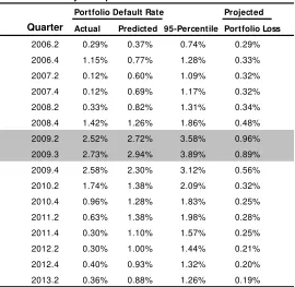
The table below shows the results for model projected portfolio loss and model predicted portfolio default rate.

probability given by the predicted portfolio level default probability. The last column shows the model projected portfolio scenario loss, reported as a percentage of the portfolio total EAD. As shown in the table below, both the model predicted and realized portfolio default rates peak at 2009.3. The projected loss peaks at 2009.2 rather than 2009.3. Note that, projected loss is not necessarily 100% concordant to the predicted default probability due to the LGD factor. The loss rate is generally higher for the entities that get hit in the first round of market shocks. As market moves further into the downturn period, more entities, including those with better risk profiles, start to default, resulting in a relatively higher portfolio default rate but slightly lower loss rate.

[image:11.612.156.426.200.463.2]

Table C. Projected portfolio default rate and loss

Portfolio Default Rate Projected

Quarter Actual Predicted 95-Percentile Portfolio Loss

2006.2 0.29% 0.37% 0.74% 0.29%

2006.4 1.15% 0.77% 1.28% 0.33%

2007.2 0.12% 0.60% 1.09% 0.32%

2007.4 0.12% 0.69% 1.17% 0.32%

2008.2 0.33% 0.82% 1.31% 0.34%

2008.4 1.42% 1.26% 1.86% 0.48%

2009.2 2.52% 2.72% 3.58% 0.96%

2009.3 2.73% 2.94% 3.89% 0.89%

2009.4 2.58% 2.30% 3.12% 0.56%

2010.2 1.74% 1.38% 2.09% 0.32%

2010.4 0.96% 1.28% 1.83% 0.25%

2011.2 0.63% 1.38% 1.98% 0.28%

2011.4 0.30% 1.10% 1.57% 0.25%

2012.2 0.30% 1.00% 1.44% 0.21%

2012.4 0.40% 0.93% 1.32% 0.20%

2013.2 0.36% 0.88% 1.26% 0.19%

Conclusion. Risk sensitivity is a key measure for a stress-testing model. In this paper, we

differentiate asset correlations between non-default ratings, and fit stress testing factor models at the rating level, targeting the downgrade risk. We thus achieve desired risk sensitivity and robustness for the stress testing models under stress scenarios. By targeting the downgrade risk rather than default risk, we address the issue of low default counts for high quality ratings. The proposed models can be fitted effectively by using, for example, SAS non-linear mixed procedure. Bootstrap aggregation technique is used to address the serial correlation issue for the time series sample. We believe the proposed approaches provide a step-by-step, effective, and practical tool for practitioners in the fields of financial stress testing.

REFERENCES

[1] Basel Committee on Banking Supervision (2009). Principles for Sound Stress Testing Practices and Supervision

http://www.bis.org/publ/bcbs155.pdf

[3] Blaschke, W., Jones , M. T., Majnoni, G., and Peria, S. M.(2001). Stress Testing of Financial Systems: An Overview of Issues, Methodologies, and FSAP Experiences, IMF Working Paper, WP/01/88

http://www.imf.org/external/pubs/ft/wp/2001/wp0188.pdf

[4] Breiman, L. (1996). Bagging Predictors. Machine Learning 24: 123-140 http://www.cs.utsa.edu/~bylander/cs6243/breiman96bagging.pdf

[5] Bunn, P. (2005). Stress testing as a tool for assessing systematic risks, Financial Stability Review, 2005:6, pp.116-126

http://www.bankofengland.co.uk/publications/Documents/fsr/2005/fsr18art8.pdf

[6] Demey, P., Jouanin, J., Roget, C, and Roncalli, T. (2004). Maximum likelihood estimate of default correlations, Risk, November 2004

http://thierry-roncalli.com/download/risk-mledc.pdf

[7] Drehmann, M. (2008). Stress tests: Objectives, challenges and modelling choices, Economic Review, 2008:Vol 60 (2), pp. 60-92

http://www.riksbank.se/Upload/Dokument_riksbank/Kat_publicerat

/Artiklar_PV/2008/drehmann2008_2_eng.pdf

[8] Friedman, J., Hastie, T., and Tibshirani, R. (2008). The Elements of Statistical Learning, 2nd edition, Springer

[9] Gordy, M. B. (2003). A risk-factor model foundation for ratings-based bank capital rule. Journal of Financial Intermediation12, pp.199-232.

[10] Gordy, M., Heitfield, E. (2002). Estimating default correlations from short panels of credit rating performance data. Federal Reserve Board Working paper, January 2002 [11] Jacobson, T., Linde, J., Roszbach, K. (2011) Firm Default and Aggregate Fluctuations, Board of Governors of the Federal Reserve System, August 2011

[12] Merton, R. (1974). On the pricing of corporate debt: the risk structure of interest rates. Journal of Finance, Volume 29 (2), 449-470

http://www.jstor.org/discover/10.2307

/2978814?uid=2129&uid=2&uid=70&uid=4&sid=21102236625247

[13] Meyer, C. (2009). Estimation of intra-sector asset correlation. The Journal of Risk Model validation, Volume 3 (3), Fall

http://www.risk.net/digital_assets/5021/jrm_v3n3a3.pdf

[14] Miu, P., Ozdemir, B. (2009). Stress testing probability of default and rating migration rate with respect to Basel II requirements, Journal of Risk Model Validation, Vol. 3 (4) Winter 2009, pp

.3-38

[15] Miu, P., Ozdemir, B. (2008). Estimating and validating long-run probability of default with respect to Basel II requirements. The Journal of Risk Model validation, Volume 2/Number 2, 3-41

http://www.risk.net/digital_assets/5008/jrm_v2n2a1.pdf

[16] Pindyck, R. S., Rubinfeld, D. L. (1998). Econometric Models and Economic Forecasts, 4th Edition, Irwin/McGraw-Hill

[17] Rosen, D., Saunders, D. (2009). Analytical methods for hedging systematic credit risk with linear factor portfolios. Journal of Economic Dynamics & Control, 33 (2009), 37-52 http://www.r2-financial.com/wp-content/uploads/2010/07/LinearFactor.pdf

[18] Sorge, M. (2004). Stress-testing financial systems: an overview of current methodologies, BIS Working papers, No. 165

[19] Tarashev, N., Borio, C., and Tsatsaronis, K. (2010). Attributing systematic risk to individual institutions,” Technical Report Working Papers No 308, BIS, May 2010.

http://www.bis.org/publ/work308.pdf

[20] Vasicek, O. (2002). Loan portfolio value. RISK, December 2002, 160 - 162.

SAS Institute Inc.

http://www.ats.ucla.edu/stat/sas/library/nlmixedsugi.pdf