Abstract Short term forecasting algorithms are widely used for prediction of vehicular traffic flows for adaptive traffic management. However, despite the increasing interest in the promotion of cycling in cities, little research has been carried out into the use of traffic forecasting algorithms for bicycle traffic. Structural time series models allow the various components of a time series such as level, seasonal and regression effects to be modelled separately to allow analysis of previous trends and forecasting. In this paper, a case study at a segregated bicycle lane in Dublin, Ireland was performed to test the forecasting accuracy of structural time series models applied to continuous observations of cyclist traffic volumes. It has been shown that the proposed models can produce accurate peak period forecasts of cyclist traffic volumes at both 1 hour and fifteen minute resolution and that the percentage errors are lower for hourly forecasts. The inclusion of weather metrics as explanatory variables had varying effects on the forecasting accuracies of the models. These results directly aid the design of traffic signal control systems accommodating cyclists.
I. INTRODUCTION
Continuous short term forecasting of traffic conditions is essential for enhancement of traffic management systems through the use of Intelligent Transport System (ITS) technologies. In the last several decades, much research interest has focused on the development of algorithms for forecasting of motor vehicle traffic [1]. However, very little research attention has been given to the development of forecasting algorithms for non-motorized modes of transport such as cycling and their integration with current ITS technologies. Encouraging cycling in cities is being increasingly recognized as an effective way of mitigating both the external costs of motorized transport such as air pollution and traffic congestion [2] and the detrimental health effects of sedentary lifestyles [3]. However, current dynamic traffic management systems are unable to make operational modifications based on observed cyclist traffic and this poses a potential limitation to the capacity of a transport network to accommodate cyclists safely and efficiently. In recent years, more cities are beginning to collect cyclist count data using technologies such as selective inductive loop detectors and pneumatic tubes and this presents an opportunity for ITS engineers to integrate intelligent management of cyclist traffic into existing traffic management systems. However, as the dynamics of bicycle
Ronan Doorley, Brian Caulfield and Bidisha Ghosh are with the Department of Civil, Structural, and Environmental Engineering, Trinity College, Dublin, Ireland (e-mail: [email protected]; [email protected]; [email protected]).
Vikram Pakrashi is with the Department of Civil and Environmental Engineering, School of Engineering, University College Cork, Ireland (email: [email protected]).
traffic are clearly different to those of motor vehicle traffic, considerable research is required in order to identify optimal forecasting algorithms.
Univariate traffic flow models may be developed by using theoretical techniques based on traffic process theory or by using empirical techniques which employ statistical and/or heuristic methods. The empirical techniques can be further classified into non-parametric and parametric approaches. The non-parametric techniques, which include artificial neural networks and non-parametric regression, do not make any assumptions regarding the functional form of the dependent and independent variables and are data intensive [4]. The parametric techniques include time series models such as Box-Jenkins models and exponential smoothing models. Structural time series models are a relatively new class of time series models which are solved in state space form and have been shown to be effective in short term forecasting of urban traffic conditions [5]. A further advantage of models in state space form is the meaningful depiction of the characteristics of the system underlying the observations such as trend and seasonality. This current study proposes the use of structural time series modelling for short term forecasting of bicycle traffic conditions.
II. THEORETICAL BACKGROUND A. State Space Models
Structural time series models are a class of time series models whereby observations are modelled as a linear combination of a vector of state variables perturbed by random disturbances [6]. These state variables represent components of a dynamic system which have direct physical interpretation such as trend, seasonal and/or slope components. In the Basic Structural Model, (BSM) described by Harvey [7], the state of the system is described by three components local level, local trend and seasonal index. A BSM with seasonal period, s can be written in the form:
(1)
(2)
(3)
(4)
=
+
+
+
=
1+
1+
=
1+
=
+
1
=1
where yt is the modeled time series, t is the observation
disturbance variance, t, t and t denote the local level, local
slope and seasonal index respectively and t, t and t are
their respective disturbance variances. If any of these disturbance variances are zero, the component is deterministic otherwise they vary stochastically. For the purpose of traffic flow modeling, it can be assumed that there is no slope component [5] and so, (1) reduces to:
(5) If the observations in a time series are thought to be dependent on external factors; explanatory variables may also be included in the BSM:
(6)
where j is a regression coefficient, xj,t is an exogenous variable and k is the total number of exogenous variables.
B. Filtering and Smoothing
In state space modelling, the Kalman filter [8] is used to recursively update the current estimates and predictions of the state variables and the observations as new data are observed. Since the BSM is a Gaussian Linear Model, all of the relevant distributions are Gaussian and so, only the means and covariances are required. The filtering values of the state variables at time t and their covariance matrix are derived from the conditional distributions of the state variables at time t given y1, y2 t. The one-step ahead
forecasts of the state variables and observations at time t and their covariance matrices are derived from the respective predictive distributions of the state variables and the observations at time t given y1, y2 t-1.The Kalman smoother is used to retrospectively update the estimates of the state variables at time t given all available observations. The smoothed values of the state variables at time t and their covariance matrix are derived from the conditional distributions of the state variables at time t given y1, y2 t T where T>t [6]. Multi-step ahead forecasts may
be obtained by continuing the Kalman filtering process and treating all observations for t>T as missing values which are easily dealt with in state space analysis [9].
III. METHODOLOGY
A. Data Collection
In this study, a univariate BSM is proposed for short term forecasting of cyclist traffic volumes. Cyclist counts from selective inductive loop detectors on a segregated cycle lane in Dublin city were used for model development and testing. The detectors are located in the South section of Dublin City Centre, along a busy section of the canal route into the city. Cyclist volumes were recorded in both away from the city center. Hourly cyclist volumes were recorded in both directions between Monday, October 3rd,
2011, 00:00 and Thursday, August 30th, 2012, 23:00.
Hourly measurements of rainfall (mm), mean wind speed (km/hr) and temperature (°C) from a nearby weather station were available for the same period and so these could be included in models as explanatory variables [10]. Fifteen minute cyclist volumes were recorded between Wednesday, September 14th, 2011, 12:30 and Thursday
April 18th, 2012, 23:45. In each case, weekends were
excluded from the analysis as different dynamics and significantly lower cyclist volumes were observed in comparison to weekdays. Exclusion of weekend data is typical in traffic modelling [5]. The observations for the final 24 hours of each series were used for evaluation of the accuracy of the models.
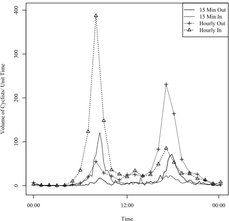
The original observations of each series for a single day, January 9th, 2012 are shown in Fig. 1 in order to clearly
daily peak corresponds to the evening rush hour between 16:00 and 19:00 w
the morning rush hour between 07:00 and 10:00. The mean ( ) and coefficient of variation (CV) for the four time series are shown in Table 1, for both peak and off-peak observations. The ratio of mean cyclist volumes during peak hours to mean cyclist volumes during off-peak hours direction. This shows that the morning peaks are more pronounced than the evening peaks. It can also be seen that the CVs are significantly higher during off-peak periods for both directions.
B. Analysis
All analysis was carried out using R [11] and the dlm
[image:2.612.315.550.482.709.2]package [6]. Maximum likelihood estimation was used to estimate the hyperparameters (disturbance variances) of models based on the data. This was carried out by using the optim function of the R base package to minimize the negative loglikelihood of the state space model as a
Figure 1. Original observations for Jan 9th, 2012
=
+
+
=
+
+
,=1
+
Time
Volume of Cyclists/ Unit Time
00:00 12:00 00:00
0
100
200
300
400 15 Min Out
TABLE I. DESCRIPTION OF PEAK AND OFF-PEAK CYCLIST VOLUMES
Direction peak CVpeak off-peak CVoff-peak
15 min Out 33.6 0.5 5.5 1.0
In 48.6 0.7 6.2 1.0
Hourly Out 139.5 0.4 22.8 0.9
In 203.5 0.6 25.6 0.8
function of the hyper-parameters, given the observed time series [6]. Once the model equations had been specified, Kalman filtering and smoothing were used to recursively update the conditional and predictive distributions of the states and observations.
IV. APPLICATION OF THE PROPOSED BSMMODEL A. BSM without Explanatory Variables
All four time series of cyclist volume observations were modelled using BSMs. Initial efforts at model building included various combinations of level, slope and seasonal index components. It was found that for all four time series, the slope components varied only slightly around near zero values and so the slope components were omitted from later models. The model chosen for all four series in this part of the study is specified by (2), (4) and (5). Table 2 shows the maximum likelihood estimates for the hyper-parameters of the four models. The seasonal disturbance variance was zero fifteen minute interval series and so this seasonal component was deterministic. All other components included in the four models were stochastic. An advantage of state space models is that they allow retrospective analysis of the behavior of the system underlying the observations. In Fig. 2, the smoothed trend, seasonal and irregular components of the two time series of sub-plots for one week from Monday, 31st October, 2011,
00:00 to Monday 7th November, 2011, 00:00. The first day, October 31st, was a public holiday in Ireland and so bicycle
traffic was unusually low and this is reflected by a sharp dip in the smoothed level component.
For the final 24 hours of each series, one-step-ahead forecasts were made for each time step and compared to the actual observations. The MAPE, RMSE and MAD for the predictions are shown in Table 3 for the peak hours, the off-peak hours and the full 24 hours. The MAPE values during the peak hours are comparable to those found with structural time series modeling of motor vehicle traffic volumes [5]. For the off-peak hours, the absolute errors are considerably lower but the MAPEs are higher. This is because there were a high proportion of near-zero observations with relatively high variance in the off-peak periods, as evidenced by the higher CV of the off-peak observations. Since MAPE normalizes the errors by the actual observations; small errors on near-zero values can cause the MAPE to increase dramatically. For this reason, high MAPEs during the off-peak periods should not be considered to be of substantial importance. The peak period MAPEs were lower for the hourly series than for the fifteen minute series, suggesting a
TABLE II. HYPER-PARAMETERS OF BSM MODELS
Direction
15 min Out 8.22 2.99 0.00
In 8.26 10.54 0.04
Hourly Out 6.63 133.13 1.32
In 32.35 235.97 12.11
trade-off between resolution and accuracy. The peak period RMSE and MAD
simply because the morning peak was more concentrated than the evening peak and so the value being predicted was greater.
Multi-step forecasts were also performed for the same periods with all predictions made from 00:00 (midnight). This means that, for the peak periods, the forecasts were 7-10 hours ahead for the In series and 16-19 hours ahead for the Out series. The mean and 95% confidence intervals for the full 24 hours of each prediction are shown in Fig. 3 along with the actual observations for the same day. In all four cases, the mean of the predictive density predicts the shape of the actual observations well. The 95% confidence intervals widen as the forecasting period increases. This is mainly due to increasing uncertainty regarding the level component. The error measures for the multi-step ahead forecasts are also shown in Table 3. Similarly to the 1-step ahead forecasts, the MAPEs were reasonably low for the peak periods but higher for the off-peak periods. When compared to the 1-step ahead forecasts, there were no significant changes in the MAPEs of the peak periods due to the longer forecasting periods for the fifteen minute series, the peak MAPE actually decreased. The peak period MAPEs of the hourly series were lower than those of the fifteen minute series, particularly in the Out direction.
T here are currently
no cyclist volume forecasting algorithms in regular use and so comparison with industry standards was not possible. The peak period multi-step ahead MAPEs for both of the hourly series are close to those found in a previous study by the authors which used a seasonal ARIMA model [12] to model cyclist volume observations at the same location [13]. However, state space models have several distinct advantages over ARIMA models which justify the increased computational load. These include the lack of a stationarity requirement and increased flexibility. Any ARIMA model may be represented in state space form but state space models may also cover a much wider range of models of varying complexity. For example, unlike ARIMA models, space models can handle explanatory variables with ease and this is explored in the next section.
B. BSM with Explanatory Variables
Figure 2. Smoothed level, seasonal and irregular components for the fifteen minute cyclist volume series ((a), (c) and (e)) and the hourly cyclist volume series ((b), (d) st October, 00:00 to Monday, 7th November, 00:00
individually and all together. The models were specified by (2), (4) and (6). The explanatory variables were lagged by one hour as this was deemed to be the most important time difference in terms of impact on the decision of whether or not to make a trip by bicycle. The smoothed values of the regression coefficients, , for both directions are shown in Table 4. Although the directions of the estimated impacts of the weather variables make qualitative sense, the 95% confidence intervals indicate that these impacts were not statistically significant, with the exception of temperature in . This does not necessarily indicate that the weather variables considered do not affect cyclist traffic volumes as the local level component would also respond to
any external factors which cause a gradual change in the level of the series.
Peak period predictions from midnight were also made for each model and the MAPEs, RMSEs and MADs are shown in Table 4. Inclusion of the explanatory variables had varying effects on the peak forecasting accuracy of the models. When rain was included as an explanatory variable in the models, all measures of error either improved or stayed the same for both directions. The inclusion of the temperature variable affected some error measures positively and some negatively in both series, with no clear pattern. When all three variables were included, all measures of error
(a)
Mon Tues Wed Thu Fri Mon
-20
0
20
40
60
80
Day
Original Smoothed Level 95% CIs
(b)
Mon Tues Wed Thu Fri Mon
-100
0
100
200
Original Smoothed Level 95% CIs
Day
(c)
Mon Tues Wed Thu Fri Mon
0
20
40
60 Smoothed Seasonal 95% CIs
Day
Volume of Cyclists /15 minutes
(d)
Mon Tues Wed Thu Fri Mon
-50
0
50
100
200
Smoothed Seasonal 95% CIs
Day
Volume of Cyclists /hour
(e)
Mon Tues Wed Thu Fri Mon
-20
-10
0
10
20 Irregular
Day
(f)
Mon Tues Wed Thu Fri Mon
-100
-50
0
50
100 Irregular
TABLE III. FORECASTING ERRORS OF BSMS WITHOUT EXPLANATORY VARIABLES
1-Step Ahead Forecasts
Cyclist Volume
Series
Direction
MAPE (%) RMSE (cyclists/hour) MAD (cyclists/hour)
Peak Hours Peak Off-Hours
24
hours Peak Hours
Off-Peak Hours
24
hours Peak Hours
Off-Peak Hours
24 hours
15 Min Out 15.5 (evening) 48.6 43.7 30.5 (evening) 11.0 14.9 23.5 (evening) 7.2 9.3 In 17.8 (morning) 42.9 39.0 26.4 (morning) 10.9 13.8 22.2 (morning) 7.5 9.4
Hourly Out 10.3 (evening) 37.6 34.2 16.0 (evening) 9.5 10.5 15.5 (evening) 6.6 7.7 In 10.8 (morning) 36.6 33.2 37.1 (morning) 10.2 16.2 29.4 (morning) 7.6 10.3
Multi-Step Ahead Forecasts
Cyclist Volume
Series Direction
MAPE (%) RMSE (cyclists/hour) MAD (cyclists/hour)
Peak Hours
Off-Peak Hours
24
hours Peak Hours
Off-Peak Hours
24
hours Peak Hours
Off-Peak Hours
24 hours
15 Min Out 19.2 (evening) 45.6 41.7 32.8 (evening) 9.6 14.7 25.8 (evening) 6.6 9.0 In 14.3 (morning) 33.9 30.9 23.7 (morning) 9.0 11.9 19.3 (morning) 6.2 7.8
Hourly Out 10.5 (evening) 28.9 26.6 17.5 (evening) 9.2 10.6 14.9 (evening) 6.2 7.3 In 13.2 (morning) 68.6 61.4 43.7 (morning) 10.9 18.5 35.2 (morning) 9.1 12.4
Figure 3. 24-hour multi-step ahead forecasts for the fifteen minute cyclist volume series (a) Out and (b) In, and the hourly series, (c) Out and (d) In.
(a)
00:00 12:00 00:00
-20
0
20
40
60
80
Time
Volume of Cyclists /15 minutes
Observations Forecasts 95% CIs
(b)
00:00 12:00 00:00
-50
0
50
100
Time
Volume of Cyclists /15 minutes
(c)
00:00 12:00 00:00
-100
0
100
200
300
Time
Volume of Cyclists /hour
(d)
00:00 12:00 00:00
-100
0
100
200
300
400
Time
TABLE IV. REGRESSION COEFFICIENTS AND 1-STEP AHEAD AND MULTI-STEP AHEAD PEAK PERIOD FORECAST ERRORS FOR BSMS INCLUDING
EXPLANATORY VARIABLES.
Direction Explanatory Variables [95% CI] MAPE (%) RMSE MAD
1-Step Multi-step 1-Step Multi-step 1-Step Multi-step
Out
None - 10.3 10.5 16.0 17.5 15.5 14.9
Rain -0.24 [-1, 0.52] 10.3 10.5 16.0 17.5 15.5 14.8
Temperature 0.53 [0.13, 0.93] 10.1 10.6 15.8 17.5 15.4 15.0
Wind -0.12 [-0.3, 0.06] 10.5 10.7 16.2 17.8 15.8 15.1
Rain Temperature
Wind
-0.09 [-0.87, 0.69] 0.55 [0.15, 0.95] -0.08 [-0.26, 0.1]
10.2 10.5 16.0 17.4 15.5 14.8
In
None - 10.8 13.2 37.1 43.7 29.4 35.2
Rain -0.43 [-1.61, 0.75] 10.7 13.1 37.1 43.5 29.4 35.0
Temperature 0.53 [-0.05, 1.11] 10.7 13.6 37.5 44.6 29.5 36.2
Wind -0.05 [-0.31, 0.21] 10.7 13.3 37.0 43.9 29.3 35.5
Rain Temperature
Wind
-0.29 [-1.47, 0.89] 0.55 [-0.05, 1.15] -0.08 [-0.34, 0.18]
10.9 13.6 37.2 44.4 29.6 36.0
. These results indicate that the effectiveness of using weather metrics as explanatory variables in BSMs in this context depends highly on the choice of variables and the pertinent measure of accuracy. Further research will be required in order to determine whether different combinations of variables, lag periods and study location may result in more consistent improvements in predictive accuracy.
V. CONCLUSION
This study has shown that structural time series modelling may be an effective tool for retrospective analysis and forecasting of bicycle traffic on segregated cycle paths. Peak period 1-step and multi-step forecasts for morning and evening rush hour periods were performed with good accuracy. Further studies are required in order to test the prediction accuracy across different locations with varying traffic conditions. The particular explanatory variables explored in this study were not found to consistently improve prediction accuracy but future work may use a similar framework to test the usefulness of other variables which may be expected to influence cyclist volumes on cycle paths. The potential for accurate short term predictions during peak traffic periods may be exploited in order to improve real-time optimization of traffic signal control systems and provide enhanced safety and priority to cyclists and to steer the network equilibrium towards conditions which make cycling the most attractive mode of transport.
ACKNOWLEDGMENT
This research was supported by the Environmental Protection Agency, Ireland.
REFERENCES
[1] E. I. Vlahogianni, J. C. Golias, and M. G. Karlaftis, "Short-term traffic forecasting: Overview of objectives and methods," Transport Reviews, vol. 24, pp. 533-557, Sep 2004.
[2] P. Bickel, R. Friedrich, A. Burgess, P. Fagiani, A. Hunt, G. D. Jong, et al., "Developing Harmonised European Approaches forTransport Costing and Project Assessment " 2006.
[3] G. Deenihan and B. Caulfield, "Estimating the health economic benefits of cycling," Journal of Transport & Health, vol. 1, pp. 141-149, 6// 2014.
[4] W. Y. Szeto, B. Ghosh, B. Basu, and M. O'Mahony, "Multivariate Traffic Forecasting Technique Using Cell Transmission Model and SARIMA Model," Journal of Transportation Engineering-Asce, vol. 135, pp. 658-667, Sep 2009.
[5] B. Ghosh, B. Basu, and M. O'Mahony, "Multivariate Short-Term Traffic Flow Forecasting Using Time-Series Analysis," Ieee Transactions on Intelligent Transportation Systems, vol. 10, pp. 246-254, Jun 2009.
[6] G. Petris, S. Petrone, and P. Campagnoli, Dynamic linear models. New York: Springer, 2009.
[7] A. C. Harvey, Forecasting, Structural Time Series Models and the Kalman Filter. Cambridge: Cambridge University Press, 1989.
[8] R. E. Kalman, "A new approach to linear filtering and prediction problems," Journal of basic Engineering, vol. 82, pp. 35-45, 1960.
[9] J. Durbin and S. J. Koopman, Time Series Analysis by State Space Methods. London, U.K.: Oxford University Press, 2001. [10] World Climate. (2012, November 7th). Available:
http://www.worldclimate.com
[11] R Core Team, "R: A Language and environment for statistical computing. R Foundation For Statistical Computing," ed. Vienna, Austria, 2013.