doi:10.4236/jgis.2011.34029 Published Online October 2011 (http://www.SciRP.org/journal/jgis)
Performance Improvement of GPS GDOP Approximation
Using Recurrent Wavelet Neural Network
Sadaf Tafazoli, Mohammad Reza Mosavi*
Department of Electrical Engineering, Iran University of Science and Technology, Tehran, Iran E-mail:*[email protected]
Received May 5, 2011; revised June 26, 2011; accepted July 14, 2011
Abstract
One of the most important factors affecting the precision of the performance of a GPS receiver is the relative positioning of satellites to each other. Therefore, it is essential to choose appropriate accessible satellites utilized in the calculation of GPS positions. Optimal subsets of satellites are determined using the least value of their Geometric Dilution of Precision (GDOP). The most correct method of calculating GPS GDOP uses inverse matrix for all combinations and selecting the lowest ones. However, the inverse matrix method, es-pecially when there are so many satellites, imposes a huge calculation load on the processor of the GPS navigator. In this paper, the rapid and precise calculation of GPS GDOP based on Recurrent Wavelet Neural Network (RWNN) has been introduced for selecting an optimal subset of satellites. The method of NNs pro-vides a realistic calculation approach to determine GPS GDOP without any need to calculate inverse matrix. Keywords:Rapid and Precise Calculation, GPS GDOP, RWNN
1. Introduction
Global Positioning System (GPS) is a satellite based po-sitioning system which was rapidly grown in the past two decades. It can cover almost all around the world, using satellite signals in order to measure accurate time, alti-tude, longitude and latitude in every desirable point on earth, sea or air as well as space.
The methods of calculating the coordinates in a GPS receiver are based on the utilizing four visible satellites in a set of visible satellites and errors may usually hap-pen when one or more satellites are invisible or the in-formation sent by them are unclear. There are various algorithms for the classification of visible satellites that can be used to classify appropriate satellites in one group. Considering the geostationary position of satellites in earth's orbit, five to eight GPS satellites are visible at any position on earth. To calculate the coordinates of that point on the earth the four-satellite groups can be used differently [1,2].
In the common algorithm used for the most GPS re-ceivers, the first selected satellite is the one whose con-necting line joining the satellite to its receiver is more vertical. After selecting the base satellite, the other three satellites are determined based on their most appropriate geometric configuration. At the beginning of locating
and after appropriate selection of four satellites accord-ing to the said algorithm, the error occurraccord-ing within a specified limit is acceptable; but the increase in the time of the original selection increases proportionally the oc-curred error. Therefore, it is required that the selection is repeated within specified intervals. To reduce the errors of calculation, it is necessary to reduce the temporal in-terval existing between the classification and frequent selections of appropriate satellites. The increase rate of calculation error after selection, and fixation of satellites depends on the different parameters including manufac-turing technology of receiver, quality of receiver, applied algorithms, and number of tracking channels. Any in-crease in tracking channels of a receiver inin-creases the ability of the receiver in selecting and classifying satel-lites. Therefore, the receivers having more tracking channels cause less error than other receivers. As the vehicles using the GPS moves, the initial selected satel-lites disappear in horizon and become invisible to the human eye. At this stage, other appropriate satellites shall be selected [3,4].
S. TAFAZOLI ET AL. 319
The use of Neural Networks (NNs) is a solution for complicated issues, for which no mathematical models are available. NNs use several simple computing units called neuron (nervous cells) patterned after the cells of human brain. The neurons of each NN process and con-vert the stimulations or input data to send them to the outputs. These outputs may be connected to the inputs of other neurons. These neurons connecting to each other form a NN. A NN consists of one input and one output layer. The data are received by a NN through its input layer and processes by all layers before receiving the output layer [6].
The objective of this paper is to suggest a rapid method for calculating GPS GDOP using the NNs. This method strongly decreases the load of GPS GDOP clas-sical method calculations for selecting an optimal subset of satellites by GPS navigator processors. This paper has been organized as follows. In the Section 2, the concept of GPS GDOP has been studied in brief. In the Sections 3, 4 and 5, the manner of rapid and precise calculation of GPS GDOP based on RWNN to select an appropriate subset of navigator satellites. To study the workability of this method, it has been tested and compared in the Sec-tion 6. Finally, the SecSec-tion 7 provides us with the con-clusion.
2. The Concept of GPS GDOP
GPS receivers report usually the geometric quality of satellites based on Position Dilution of Precision (PDOP). PDOP shows the vertical and horizontal DOP, i.e. geo-graphical longitude, latitude, and altitude. Low DOP increases and high DOP decreases the probability of pre-cision. If the sides of the pyramid formed by four satel-lites are almost equal (equiangular pyramid), this con-figuration leads to an appropriate GPS GDOP and vice versa. GPS GDOP is a very effective tool for GPS. All receivers use the algorithms based on GPS GDOP to find the best subset of visible satellites used for tracking. To locate satellites, azimuth (AZ) and angle of elevation ( ) can be used. To define the concept of GPS GDOP, it is helpful to use sample calculations expressing a compromise between precision and the position of satel-lite. For this purpose, the matrix of
E
H is defined as follows [7]:
Cos( 1) * Sin( 1) Cos( 1) * Cos( 1) Sin( 1) 1 Cos( 2) * Sin( 2) Cos( 2) * Cos( 2) Sin( 2) 1 Cos( 3) * Sin( 3) Cos( 3) * Cos( 3) Sin( 3) 1 Cos( 4) * Sin( 4) Cos( 4) * Cos( 4) Sin( 4) 1
E Az E Az E
E Az E Az E
H
E Az E Az E
E Az E Az E
(1) GPS GDOP shall be defined as follows:
1 trace[adj( )]
GDOP trace( )
det( )
T T
T H H H H
H H
(2)
GPS GDOP provides us with a simple interpretation of the fact that how much a unit of measurement error par-ticipates in the occurrence of positioning error for a specified position, and it determines the factor of meas-urement noise amplitude.
3. Rapid and Precise Calculation of GPS
GDOP Using Neural Networks
To prepare experimenting data, all input and output variables are normalized within an interval of [0,1] to reduce the experimenting time. whereas, H HT is a 4 × 4 matrix, it has four eigenvalues i
We know that four eigenvalues for the matrix of (i1, 2, 3, 4).
T
1H H is equal to i1
. Considering that the trace of a matrix is equal to the sum of its eigenvalues, the fol-lowing equation is formed as follows [8]:
1 1 1
1 2 3 4
GDOP 1
(3) The mapping with the definition of four variables is as follows:
1 1 2 3 4 trace( )
T
x H H (4)
2 2 2 2 2
1 2 3 4
2 trace T
x (H H)
H
(5)
3 3 3 3 3
31 234 trace ( )
T
x H (6)
4 1 2 3 4 det( )
T
x H H (7)
GPS GDOP can be shown as a functional mapping of from
4
R R1 f directly to GPS GDOP; i.e.
1 fn f
:
Input:
1, 2, 3, 4
T
x x x x
Output: yGPS GDOP
The mapping from
f
to GPS GDOP is strictly non-linear and cannot be determined analytically, but it can be approximated using a NN. The NN used in this paper has been designed for the mapping offrom
4 1
R R
f
to GPS GDOP. The Figure 1 shows the overall diagram block of GPS GDOP approximation using NNs including Recurrent NN (RNN), Wavelet NN (WNN), and Recurrent Wavelet NN (RWNN).
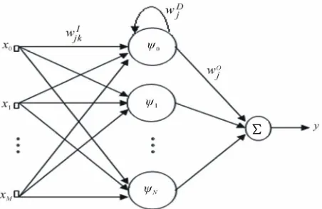
4. RWNN Architecture
Figure 1. The overall diagram block of GPS GDOP approximation using NNs.
Figure 2. RWNN architecture with (M + 1, N + 1, 1) struc-ture.
weighted sum of several wavelets. The hidden layer is composed of finite number of wavelets representing the signal.
The components of the proposed RWNN essentially include: xk-value of the k-th input neuron; j-output of.the j-th hidden.neuron; wIjk-interconnection weight between the k-th input neuron and j-th hidden neuron;
O j
w -interconnection weight between the
j
-th hidden neuron and the output neuron; wDj -recurrent weight forj
-th hidden neuron.The net internal activity of neuron
j
at time n, is given by:)] 1 ( [ , )
( ) ( 0 )
(
wIjk nxk n wDj abnetj n
M k n j
net (8)
where, net nj( ) is the sum of input to the
j
-th recurrent neuron, , j is the output of the -th recur-rent neuron and is computed by passing through the wavelet function( )n
a b net
j
( ) j net n , (.)
a b j
, obtaining:
,
( ) ( ) ( )
( ) j j a b j
j
net n b n
net n
a n
(9)
where, and are the dilation and transla-tion coefficients of the -th wavlon in hidden layer, respectively. The RWNN output of the Figure 2 network is computed:
( )
j
a n b nj( )
j
,
0
( ) N
O
j a b j J
y n w n net n
(10)The wavelet function which we have considered here is the called “Gaussian-derivative” function as:
2 1 2 ( )x xe x
(11)
5. Learning Algorithm for RWNN
The basic principle of the RWNN is to use the gradient steepest descent method to minimize the cost function. The training of RWNN is traditionally based on minimi-zation of the cost function. Suppose a set of training samples is available, the problem can be characterized as choosing the weights (or coupling strengths) of a given network such that the following total squared error is minimized [9]:
∑
22
1 1
( ) ( ) ( ) ( )
2 2
E n e n d n y n
(12) where and represent the desired and actual output of the output neuron, respectively. is a time varying error. The output weights can be adjusted ac-cording to:( )
d n y n( )
( )
e n
, ( )
( 1) ( )
( )
( )
( ) ( ) ( ) ( )
( )
O O
j j O
j
O O
j O j a
j
E n
w n w n
w n
y n
w n e n w e n net n
w n
b j
(13) where, is a learning rate. The recurrent weights are updated as follow:
( ) ( )
( 1) ( ) ( ) ( )
( ) ( )
D D D
j j D j D
j j
E n y n
w n w n w n e n
w n w n
(14) To determine the partial ( )
( ) D j y n w n
derivative, is
dif-ferentiated the network dynamics with respect to as follow:
( ) D j w n
, [ ( )]
( )
( )
( ) a b j O
j
D D
j j
net n y n
w n
w w
n (15)
where , ( )
( ) a b j
D j
net n
w n
[image:3.595.60.286.254.401.2]S. TAFAZOLI ET AL. 321
for differentiation, obtaining:
, , , [ ( )] [ ( )] ( ( ) ( ) ( ) ( ) ( ) ( )
a b j a b j j
D D
j
j j
j a b j D
j
net n net n net n
net n
w n w n
net n net n w n ) (16) Or: , , , , ( ) ( ) ( ) ( ) ( 1)
( 1) ( )
( ) a b j a b j
D
j j
a b j D
a b j j D
j
net n net n
a n w n
net n
net n w n
w n (17)
Equation (17) is non-linear dynamic recursive equa-tion and can be solved recursively with given initial con-dition as: , (0) 0 (0) a b D j w
(18)
The inputs weight can be adjusted as follow:
,
( )
( 1) ( )
( ) ( ) ( ) ( ) ( ) ( ) ( ) ( ) ( ) ( ) I I
jk jk I
jk
I
jk I
jk
a b j
I O
jk j I
jk
E n
w n w n
w n
y n
w n e n
w n
net n
w n e n w n
w n (19)
where , ( )
( ) a b j
I jk net n w n
is obtained as:
, , , , , ( ) ( ) ( ) ( ) ( ) ( ) ( ) ( ) ( )
( ) ( 1)
( ) ( )
( ) ( )
a b j a b j j
I I
j
jk jk
j
a b j I
jk
a b j D a b j
k j I
j jk
net n net n net n
net n
w n w n
net n net n
w n
net n net n
x n w n
a n w n
(20) With initial conditions:
, (0) 0 (0) a b I jk w
(21)
The translation coefficient of the -th wavlon in hidden layer can be adjusted according to:
j
' , ( ) ( 1) ( )
( ) ( ) ( ) ( ) ( ) 1 ( ) ( ) ( ) [ ( )] ( ) j j j j j O
j j a b j
j
b E n
b n b n
b n
y n
b n e n
n
b n e n w n net n
a n
(22)The dilation coefficient of the -th wavlon in hidden layer is updated as follow:
j
'
, 2
( )
( 1) ( )
( ) ( ) ( ) ( ) ( ) ( ) ( ) ( ) ( ) ( ) [ ( )] ( ) j j j j j j j O
j j a b j
j E n
a n a n
a n y n a n e n
a n
net n b n a n e n w n net n
a n (23)
6. Testing the Proposed Method
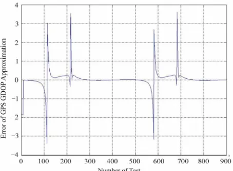
[image:4.595.57.539.68.719.2]The parameters of the proposed NNs have been opti-mized on the test data based on try and error method. Figure 3 shows the approximation error values using RWNN for 900 data.
The Table 1 shows four significant statistical charac-teristics of approximation error including maximum, minimum, average, and RMS for the approximation of GPS GDOP for 900 test data using RWNN.
[image:4.595.67.288.102.262.2]The approximation with RNN and WNN has been done and the comparative results have been shown in Table 2. Root Mean Square (RMS) was used to evaluate approximations results [10]. RMS value is computed using:
2Real NN 1
1
RMS GDOP GDOP
i T i
T (24)
where T is number of tests.
As it is visible over this Table, the RWNN is more
Table 1. Maximum, minimum, average and RMS error for the approximation of GPS GDOP for 900 test data deter-mined using RWNN.
Parameters Value Maximum 3.5928 Minimum -3.4024 Average 0.0544
RMS 0.4590
Table 2. Comparison of RNN, WNN and RWNN perform-ance for GPS GDOP approximation.
[image:4.595.58.288.355.691.2] [image:4.595.342.510.610.660.2]Figure 3. The approximation error values of GPS GDOP determined based on RWNN for 900 data with (4, 3, 1) structure.
Table 3. Comparison CPU time of classical method and NN approach for GPS GDOP approximation.
Model Name CPU Time [msec.]
Matrix inversion method 1.080 NN approach 0.029
efficiency in comparing with RNN and WNN; this is because of the RMS approximation error shortage over them.
Table 3 presents the comparison CPU time of classi-cal method and NN approach for GPS GDOP approxi-mation. The simulation results demonstrate that NN ap-proach is accurate and faster than classical method.
7. Conclusions
In this paper, the rapid and precise calculation of GPS GDOP using RWNN has been studied for the selection of an appropriate subset of navigator satellites. The method of NNs is a realistic computing approach used for the calculation of GPS GDOP without any need to inverse matrix, which imposes a huge computing load on the processor of the navigator. The performance of the proposed NN has been studied on the test data of the paper. The results show that the proposed method is fully
capable to select an optimal subset of GPS satellites with the best geometric configuration. The results of simula-tion show that the efficiency of RWNN is better than RNN and WNN.
8. References
[1] R. Yarlagadda, I. Ali, N. Al-Dhahir and J. Hershey, “GPS GDOP Metric,” IEE Proceedings—Radar, Sonar and Navigation, Vol. 147, No. 5, 2000, pp. 259-264.
doi:10.1049/ip-rsn:20000554
[2] M. Zhang and J. Zhang, “A Fast Satellite Selection Algo-rithm: Beyond Four Satellites,” IEEE Journal of Selected Topics in Signal Processing, Vol. 3, No. 5, 2009, pp. 740-747. doi:10.1109/JSTSP.2009.2028381
[3] D. Simon and H. El-Sherief, “Navigation Satellite Selec-tion Using Neural Networks,” Journal of Neurocomput-ing, Vol. 7, 1995, pp. 247-258.
doi:10.1016/0925-2312(94)00024-M
[4] M. R. Mosavi, “High Performance Methods for GPS GDOP Approximation Using Neural Network,” Journal of Geoinformatics, Vol. 4, No. 3, 2008, pp. 9-16.
[5] D. J. Jwo and C. C. Lai, “Neural Network-Based Geome-try Classification for Navigation Satellite Selection,”
Journal of GPS Navigation, Vol. 56, No. 2, 2003, pp. 291-304. doi:10.1017/S0373463303002200
[6] M. R. Mosavi, “GPS Receivers Timing Data Processing using Neural Networks: Optimal Estimation and Errors Modeling,” Journal of Neural Systems, Vol. 17, No. 5, 2007, pp. 383-393. doi:10.1142/S0129065707001226 [7] B. W. Parkinson, “Global Positioning System: Theory and
Applications,” The American Institute of Aeronautics and Astronautics, Vol. 1, 1996.
[8] D. J. Jwo and C. C. Lai, “Neural Network-Based GPS GDOP Approximation and Classification,” Journal of GPS Solutions, Vol. 11, No. 1, 2007, pp. 51-60.
doi:10.1007/s10291-006-0030-z
[9] M. R. Mosavi, “An Adaptive Correction Technique for DGPS using Recurrent Wavelet Neural Network,” IEEE Conference on Systems, Man, and Cybernetics, 2007, pp. 3029-3033. doi:10.1109/ICSMC.2007.4413579