A Clustering Algorithm for Key Frame Extraction Based on Density Peak

ISSN Online: 2327-5227 ISSN Print: 2327-5219

DOI: 10.4236/jcc.2018.612012 Dec. 26, 2018 118 Journal of Computer and Communications

A Clustering Algorithm for Key Frame

Extraction Based on Density Peak

Hong Zhao

, Tao Wang

, Xiangyan Zeng

1_{School of Computer and Communication, Lanzhou University of Technology, Lanzhou, China} 2_{Department of Mathematics and Computer Science, Fort Valley State University, Fort Valley, GA, USA}

Abstract

Aiming at the problem of video key frame extraction, a density peak cluster-ing algorithm is proposed, which uses the HSV histogram to transform high-dimensional abstract video image data into quantifiable low-dimensional data, and reduces the computational complexity while capturing image fea-tures. On this basis, the density peak clustering algorithm is used to cluster these low-dimensional data and find the cluster centers. Combining the clus-tering results, the final key frames are obtained. A large number of key frame extraction experiments for different types of videos show that the algorithm can extract different number of key frames by combining video content, overcome the shortcoming of traditional key frame extraction algorithm which can only extract a fixed number of key frames, and the extracted key frames can represent the main content of video accurately.

Keywords

Key Frame, Clustering Algorithm, HSV Color Histogram

1. Introduction

With the rapid development of multimedia and Internet technology, we are in the era of data explosion. At every moment, there are a lot of data generating such as video, text, images, blogs in all walks of life. Vivid digital video has gradually replaced the monotonous text information, which has become one of the main ways for people to spread information. Either personalized recom-mendation or content-based video retrieval, it is difficult to analyze a large amount of video data. Key frames are video pictures that can represent the main content of video simply and effectively, they provide a suitable abstraction and framework for video indexing, browsing and retrieval. The use of key frames How to cite this paper: Zhao, H., Wang,

T. and Zeng, X.Y. (2018) A Clustering Algorithm for Key Frame Extraction Based on Density Peak. Journal of Computer and Communications, 6, 118-128.

https://doi.org/10.4236/jcc.2018.612012

DOI: 10.4236/jcc.2018.612012 119 Journal of Computer and Communications greatly reduces the amount of data required in video browsing and provides an organizational framework for dealing with video content [1]. Key frame extrac-tion has been recognized as one of the important research issues in video infor-mation retrieval [2].

Clustering algorithm is the process of dividing a set of data objects into mul-tiple groups or clusters, which makes the objects in the same cluster have high similarity and the similarity of objects between different clusters is extremely low. From the point of view of pattern recognition, clustering is the discovery of potential patterns in data, helping people to group and classify them to achieve a better understanding of the distribution of data. As a kind of data mining tool, clustering analysis has been widely used in many fields such as biology, informa-tion security, intelligent business and web searching. Different clustering algo-rithms are based on different assumptions and data types, and each clustering algorithm has its limitations and biases. The choice of clustering algorithm often depends on the type of data and the purpose of clustering. For example, some clustering algorithms may work better on one application scenario, but not in another. Clustering algorithm is used to extract video key frames, and the frame images with high similarity in the video are clustered into one class, and these cluster centers are key frames.

Density-based clustering method classifies areas with sufficient high density into clusters, looking for high-density areas separated by low-density areas, and clusters with arbitrary shape can be easily obtained. The density peak clustering algorithm DPCA (clustering by fast search and find of density peaks) [3] is a new density-based clustering algorithm, which can find clusters with different densities by visualized method, quickly find the density peak points (i.e. cluster centers) of data sets, and efficiently allot sample points and eliminate outliers [4].

DOI: 10.4236/jcc.2018.612012 120 Journal of Computer and Communications large. All the image data has to be loaded into memory for calculation, so it is not only computationally large, but also prone to memory leaks. In view of this, this paper proposes a density peak clustering algorithm which combines the characteristics of HSV histogram, uses the HSV histogram to simplify calcula-tion and effectively improves the quality and efficiency of key frame extraccalcula-tion.

2. HSV Histogram Method

2.1. RGB Color Model

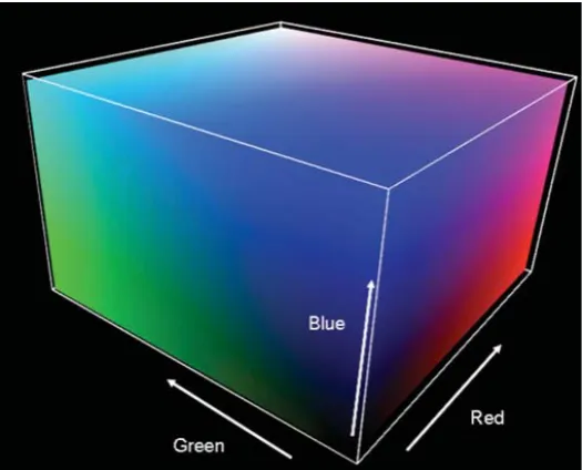
According to the tricolor theory, the human eye is more sensitive to red, green and blue, and the majority of colors can be synthesized by different proportions of red, green and blue. The RGB color space is shown in Figure 1. Any color light in nature can be mixed by adding R, G and B three primary colors in dif-ferent proportions. For instance, when the three primary components are all ze-ro, they are mixed into black light, and when the three primary components are both the maximum, they are mixed into white light. Therefore, any color cor-responds to a point in the RGB color space.

RGB color model is the most commonly used color model in image processing. As far as editing images are concerned, it is the best color model. Its physical meaning is clear and suitable for the work of color kinescope, but it does not adapt to the visual characteristics of human beings and does not con-form to the visual judgment of human eyes on color. For a color, the human eye is most concerned about its chroma, depth, brightness, and synthesizes three parameters to evaluate the color. People without professional knowledge of color cannot directly judge these colors by RGB value, so RGB color space is not in line with people’s perception of color psychology [7]. In addition, the RGB color space is uneven, so the visual difference between two colors cannot be expressed directly by the distance between two color points in the color space [8].

DOI: 10.4236/jcc.2018.612012 121 Journal of Computer and Communications

2.2. HSV Color Model

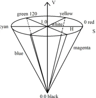
HSV color space is a color model oriented to visual perception, in which the color perception of human eye mainly includes three elements: hue, saturation and value [9]. The HSV color model corresponds to a conical subset in the cy-lindrical coordinate system, as shown in Figure 2. The V-axis represents bright-ness, the distance from the V-axis represents saturation S, and the angle of rota-tion around the V-axis represents hue H. The top surface of the cone corres-ponds to V =1_{, and the color with the maximum brightness and saturation is} located on the circumference of the top surface of the cone [10]. Androutsos et al. roughly divided the HSV color space by experiment: the areas with brightness greater than 75% and saturation greater than 20% were bright color areas, the areas with brightness less than 25% were black areas, the areas with brightness greater than 75% and saturation less than 20% were white areas, and the others were color areas [11]. The HSV model is similar to the painter’s method of color matching. By changing the color intensity and depth, different tones of a pure color can be obtained. That is, adding white to a pure color to change the color intensity and adding black to change the color depth. It can be seen that the three elements of hue, saturation and brightness in the HSV color space have a clear structure, are easy to understand and closely related to the way people feel the color. In order to capture the features of video frames better, this paper uses HSV color model to carry out subsequent experimental analysis.

2.3. HSV Histogram

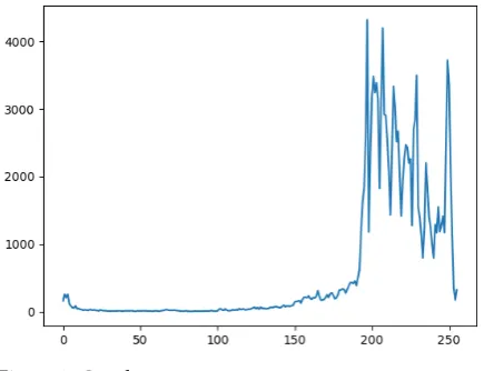
Color histogram is a widely used color feature in image processing, which de-scribes the proportion of different colors in the entire image, and does not care about the spatial location of each color [12]. As shown in Figure 3, the gray his-togram is to count all the pixels in the image and get a unified concept of the overall gray level. Among them, the horizontal axis represents the grayscale val-ue (generally taken 0 - 255), and the vertical axis is the number of pixels corres-ponding to each gray value in the image.

DOI: 10.4236/jcc.2018.612012 122 Journal of Computer and Communications

Figure 3. Gray histogram.

Choosing the appropriate number of color cells (i.e. bin of histogram) and color quantization methods are related to the performance and efficiency re-quirements of specific applications. In general, the more color intervals there are, the stronger the histogram’s ability to distinguish colors. However, color histograms with many intervals not only increase the computational burden, but are also not conducive to indexing in large image database. Moreover, for some applications, the use of very fine color space partitioning method may not nec-essarily improve the retrieval effect, especially for those applications that cannot tolerate the omission of relevant images.

In the HSV color model, it is necessary to draw the histogram of its three components (H, S, V) separately, and when there are quite a few colors in the picture, the dimension of each histogram will be higher, so the HSV color space needs quantifying first. According to the characteristics of HSV color model, the following treatments are made in this study:

1) Considering the human visual resolution ability, the hue H component is divided into 12 parts, and the saturation S and value V components are divided into 5 equal parts.

2) Considering the value range of each component and the subjective color perception, the following quantization is performed.

0 [346,15]

1 [16,45]

2 [46,75]

3 [76,105] 4 [106,135] 5 [136,165] 6 [166,196] 7 [196,225] 8 [226,255] 9 [256,285]

10 [286,315]

11 [316,345]

H H H H H H H H H H H H H ∈   _∈   ∈  _∈   _∈  ∈  =  _∈   _∈  ∈   _∈  ∈   _∈  ,

0 [0,0.2]

1 [0.2,0.4]

2 [0.4,0.6]

3 [0.6,0.8]

4 [0.8,1]

H H S H H H ∈   _∈  =_ ∈  _∈  ∈  ,

0 [0,0.2]

1 [0.2,0.4]

2 [0.4,0.6]

3 [0.6,0.8]

4 [0.8,1]

DOI: 10.4236/jcc.2018.612012 123 Journal of Computer and Communications 3) Based on the perceptual characteristics of human eyes to color, that is, the sensitivity of human eyes to the H component is greater than the S component, the sensitivity to the S component is greater than the V component, and then these three color components are merged into one-dimensional feature vectors, as shown in Equation (1).

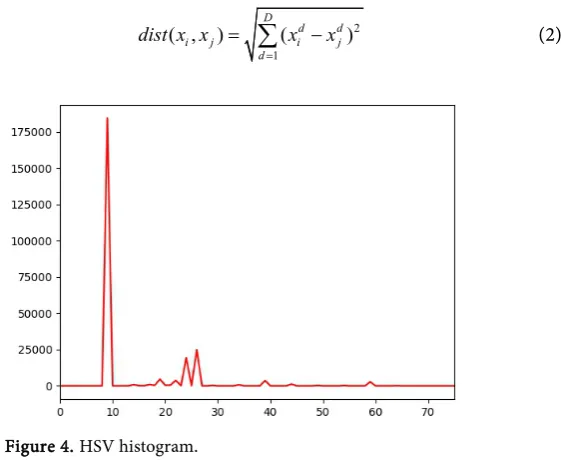
5 3 2

F= H+ S+ V ₍₁₎ Therefore, the value range of F is 0 - 75. As shown in Figure 4, a frame of video is converted into a histogram of 76 bin, in which the horizontal axis represents 76 dimensions of one-dimensional feature vector F and the vertical axis represents the number of pixels appearing on each dimension in an image.

3. Density Peak Clustering Algorithm

The main idea of density clustering algorithm is to find high density regions se-parated by low density regions. DPCA, a density peak clustering algorithm, can use visualization to help find clusters with different densities. It requires that each cluster has a maximum density point as the cluster center, each cluster cen-ter attracts and connects the points with lower density around it, and different cluster centers are relatively far away [2]. That is, the density peak clustering al-gorithm is based on two assumptions: 1) the density of cluster centers is greater than that of their neighbors, and 2) the distance between different cluster centers and the higher density point is relatively large. Therefore, there are two main quantities that need to be calculated: local density ρi and distance from higher

density points δi.

3.1. Distance Metric

Every data object has 76-dimensional attribute values, which can be expressed as 1

{ , , , ,d D} i i i i

x = x  x  x (that D = 76). The distance between sample point xi

and xj is calculated by Euclidean distance, as shown in Equation (2).

2 1

( , ) D( d d)

i j i j d

dist x x x x

=

=

∑

DOI: 10.4236/jcc.2018.612012 124 Journal of Computer and Communications

3.2. Local Density

The local density ρi of the data object xi is defined as follows:

( ( , ) )

j

i i j cutoff x U

dist x x dist

ρ χ

∈

=

∑

where χ( )x _{is an indicator function, which is defined as follows:} 1 0

( )

0 0

x x

x

χ =  ≤_>



The distcutoff item indicates the cutoff distance, and in literature [2], it is pointed out that the value range of empirical parameter t∈[1% 2%] . The distance between any two data objects in dataset U is calculated and sorted in-crementally, the value of distcutoff takes the numeric value at the t position in the incremental sequence. The local density formula describes that the local den-sity ρi of each data object xi is equal to the number of data points where the

distance from the object xi is less than the cutoff distance distcutoff .

3.3. Distance from Higher Density Points

The distance δi from higher density point of data object xi is defined as

fol-lows:

,

:

max ( ( , ))

min ( ( , )) otherwise

j

j i

i j i j

x U j i i

i j

j

dist x x

dist x x

ρ ρ

ρ ρ

δ ∈ ≠

>

≥ ∀ 

 = 

 (4)

When the local density ρi of data object xi is the global maximum value,

the relative distance δi is the maximum distance between any other data object

j

x and xi. Otherwise, some data objects xj whose local density is greater than ρi are found, and the relative distance δi is the minimum distance

be-tween data objects xj and xi.

It can be seen that DPCA aims to find data objects with large local density and relative distance as cluster centers. These cluster centers attract and connect the points with low density around them, and they are relatively far away from each other. The local density ρi and relative distance δi of each data object xi

are calculated, and a two-dimensional decision map is generated based on these two attribute values, where the horizontal axis is the local density ρi and the

vertical axis is the relative distance δi. Some data points in the upper-right

corner of the decision map can represent different cluster centers because of their high local density and large relative distance from other clusters.

4. Experimental Results

4.1. Video Frames Processing with HSV Histogram

DOI: 10.4236/jcc.2018.612012 125 Journal of Computer and Communications

F on one channel according to Equation (1) (F∈[0,75]).Then the number of pixels appearing on each HSV color level F is counted based on the HSV histo-gram method, and each frame of the video is converted into a HSV histohisto-gram, which is expressed as a 76-dimensional eigenvector in numerical form, that is

1

{ , , , ,d D} i i i i

x = x  x  x (D = 76).

4.2. DPCA Clustering Process

Each frame of the video has been converted into a 76-dimensional feature vec-tor, so the size of the input data is 511 76× _{. The distance of any two sample} points is calculated according to the distance metric Equation (2) and stored in the distance matrix M, which is a 511 511× _{symmetric matrix. The value on} the diagonal line of matrix M is all zero, M i j[ , ] corresponds to the distance between data object xi and xj, and M i j[ , ]=M j i[ , ].

The empirical parameter t∈[1% 2%]∼ , and some experiments has been car-ried out at t=1% _and t=2% _{respectively. The distance of any two data} ob-jects in dataset U is calculated and sorted incrementally, the value of distcutoff takes the numeric value at the t position in the incremental sequence. Therefore, the larger t is, the larger the cutoff distance dcutoff is, and the greater the local density ρi of data object xi is. The experimental results are shown in Table

1.

Next, the local density ρi of each data object xi is calculated using the

density calculation Equation (3), and the relative distance δi of each data

ob-ject xi is calculated with the relative distance calculation Equation (4). Finally,

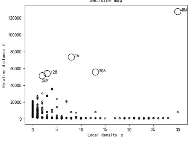
the decision map is generated. Figure 5 and Figure 6 are decision maps when t = 1% and t = 2% respectively.

DOI: 10.4236/jcc.2018.612012 126 Journal of Computer and Communications

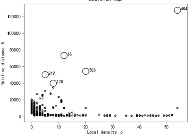
Figure 6. Decision maps corresponding to t = 2%.

Table 1. Effect of empirical parameter t on cutoff distance.

t dcutoff

1% 1766.30

1.5% 2419.76

2% 3196.17

When t takes different values, the local density and relative distance of each sample point and the distribution of sample points on decision maps will be dif-ferent. In order to make the local density of data sample large, t = 2% was adopted as the experimental scheme in this study. In Figure 6, the sample point 484 in the upper right corner has the maximum local density, which indicates that the number of sample points similar to the sample point 484 in dataset U is the largest. In addition, sample points 16 and 306 have large local density and relative distance, they can also be selected as cluster centers. These three cluster centers can represent different clusters, and their corresponding video frames are also strong representative. Therefore, the 16, 306 and 484 frames of the video are key frames.

DOI: 10.4236/jcc.2018.612012 127 Journal of Computer and Communications

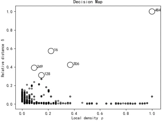
Figure 7. Normalized decision maps corresponding to t = 2%. Table 2. Local density and relative distance of five cluster centers.

Frame ρi δi

16 12 73,045.71

128 8 39,697.45

249 5 49,962.86

306 20 53,948.63

484 54 127,402.09

Since this study is mainly to find the key frames of video, it is not concerned about which sample points are included in every cluster, so it is only necessary to examine whether each sample point has potential to be a cluster center. In order to prevent the influence of different attributes during the experiment, the nor-malization of local density ρi and relative distance δi can be considered. The

normalized decision map is shown in Figure 7.

5. Conclusion

DOI: 10.4236/jcc.2018.612012 128 Journal of Computer and Communications can form clusters with arbitrary shape without the need to set up the initial pa-rameters artificially.

Acknowledgements

This work was supported by the Natural Science Foundation of China under Grant Nos. 51668043 and 61262016 and the Gansu Natural Science Foundation of China under Grant No.18JR3RA156.

Conflicts of Interest

The authors declare no conflicts of interest regarding the publication of this pa-per.

References

[1] University, T. (2012) Key Frame Extraction Using Unsupervised Clustering Based on a Statistical Model. Tsinghua Science & Technology, 10, 169-173.

[2] Cao, C.Q. (2012) Research on Key Frame Extraction in Content-Based Video Re-trieval. M.S. Thesis, Taiyuan University of Technology, Taiyuan.

[3] Rodriguez, A. and Laio, A. (2014) Machine Learning. Clustering by Fast Search and Find of Density Peaks. Science, 344, 1492. https://doi.org/10.1126/science.1242072 [4] Zhang, J.Q. and Zhang, H.Y. (2017). Clustering by Fast Search and Find of Density

Peaks Based on Manifold Distance. Computer Knowledge & Technology, 13, 179-182.

[5] Jiang, L.C., Shen, G.Q. and Zhang, G.X. (2009) Image Retrieval Algorithm Based on HSV Block Color Histogram. Mechanical and Electrical Engineering, 26, 54-57. [6] Zhuang, Y.T., Rui, Y., Huang, T.S. and Mehrotra, S. (2002) Adaptive Key Frame

Extraction Using Unsupervised Clustering. International Conference on Image Processing.

[7] Wei, B.G. and Li, X.Y. (1999) Research Progress of Color Image Segmentation.

Computer Science, 4, 59-62.

[8] Xu, X.U. (1999) A Method of Dominant Colors Extraction and Representation for CBIR Systems. Journal of Computer Aided Design & Computer Graphics, 11, 385-388.

[9] Zhang, Y.J. (2012) Image Engineering: Image Analysis. 2nd Edition, Tsinghua Uni-versity Press.

[10] Castleman, K.R., Zhu, Z.G. and Lin, X. (2002) Digital Image Processing. 3rd Edi-tion, Electronics Industry Press.

[11] Androutsos, D., Plataniotis, K.N. and Venetsanopoulos, A.N. (1999) A Novel Vec-tor-Based Approach to Color Image Retrieval Using a Vector Angular-Based Dis-tance Measure. Elsevier Science Inc.

[12] Wu, C.Y., Tai, X.Y. and Zhao, J.Y. (2004) Image Retrieval Based on Color Features.