So close, so different : characterization of the K2 36 planetary system with HARPS N

& February 7, 2019

So close, so different: characterization of the K2-36 planetary

system with HARPS-N

M. Damasso

, L. Zeng

, L. Malavolta

, A. Mayo

, A. Sozzetti

, A. Mortier

, L. A. Buchhave

, A. Vanderburg

,

M. Lopez-Morales

_{, A. S. Bonomo}

_{, A. C. Cameron}

_{, A. Co}

_ffi

_net

_{, P. Figueira}

_{, D. W. Latham}

_{, M. Mayor}

_{, E.}

Molinari

, F. Pepe

, D. F. Phillips

, E. Poretti

, K. Rice

, S. Udry

, and C.A. Watson

1 _{INAF - Osservatorio Astrofisico di Torino, Via Osservatorio 20, I-10025 Pino Torinese, Italy}

e-mail:mario.damasso@inaf.it

2 _{Department of Earth and Planetary Sciences, Harvard University, Cambridge, MA 02138} 3 _{INAF - Osservatorio Astronomico di Padova, Vicolo dell’Osservatorio 5, 35122 Padova, Italy}

4 _{Dipartimento di Fisica e Astronomia “Galileo Galilei", Universita’di Padova, Vicolo dell’Osservatorio 3, 35122 Padova, Italy} 5 _{UC Berkeley Astronomy Department, Berkeley, CA 94720-3411}

6 _{Astrophysics Group, Cavendish Laboratory, University of Cambridge, JJ Thomson Avenue, Cambridge CB3 0HE, UK} 7 _{DTU Space, National Space Institute, Technical University of Denmark, Elektrovej 327, DK-2800 Lyngby, Denmark} 8 _{Department of Astronomy, The University of Texas at Austin, 2515 Speedway, Stop C1400, Austin, TX 78712} 9 _{Harvard-Smithsonian Center for Astrophysics, 60 Garden Street, Cambridge, MA 02138, USA}

10 _{NASA Sagan Fellow}

11 _{Centre for Exoplanet Science, SUPA, School of Physics and Astronomy, University of St Andrews, St Andrews KY16 9SS, UK} 12 _{Observatoire de Genève, Université de Genève, 51 ch. des Maillettes, 1290 Sauverny, Switzerland}

13 _{European Southern Observatory, Alonso de Cordova 3107, Vitacura, Santiago, Chile}

14 _{Instituto de Astrofísica e Ciências do Espaço, Universidade do Porto, CAUP, Rua das Estrelas, 4150-762 Porto, Portugal} 15 _{INAF – Osservatorio Astronomico di Cagliari, Via della Scienza 5 - 09047 Selargius CA, Italy}

16 _{INAF - Fundación Galileo Galilei, Rambla José Ana Fernandez Pérez 7, 38712 Breña Baja, Spain} 17 _{INAF-Osservatorio Astronomico di Brera, Via E. Bianchi 46, 23807 Merate, Italy}

18 _{Centre for Exoplanet Science, University of Edinburgh, Edinburgh, UK}

19 _{Astrophysics Research Centre, School of Mathematics and Physics, Queen’s University Belfast, BT7 1NN, Belfast, UK}

ABSTRACT

Context.K2-36 is a K dwarf orbited by two small (Rb=1.43±0.08R⊕andRc=3.2±0.3R⊕), close-in (ab=0.022 AU andac=0.054

AU) transiting planets discovered by the Kepler/K2 space observatory. They are representatives of two distinct families of small planets (Rp<4R⊕) recently emerged from the analysis of Kepler data, with likely a different structure, composition and evolutionary

pathways.

Aims.We revise the fundamental stellar parameters and the sizes of the planets, and provide the first measurement of their masses and bulk densities, which we use to infer their structure and composition.

Methods.We observed K2-36 with the HARPS-N spectrograph over∼3.5 years, collecting 81 useful radial velocity measurements. The star is active, with evidence for increasing levels of magnetic activity during the observing time span. The radial velocity scatter is∼17 m s−1_{due to the stellar activity contribution, which is much larger that the semi-amplitudes of the planetary signals. We tested}

different methods for mitigating the stellar activity contribution to the radial velocity time variations and measuring the planet masses with good precision.

Results.We found that K2-36 is likely a∼1 Gyr old system, and by treating the stellar activity through a Gaussian process regres-sion, we measured the planet massesmb=3.9±1.1M⊕andmc=7.8±2.3M⊕. The derived planet bulk densitiesρb=7.2+2−2..51 g cm

−3_and

ρc=1.3+0−0..75 g cm

−3_{point out that K2-36 b has a rocky, Earth-like composition, and K2-36 c is a low-density sub-Neptune.}

Conclusions.Composed of two planets with similar orbital separations but different densities, K2-36 represents an optimal laboratory for testing the role of the atmospheric escape in driving the evolution of close-in, low-mass planets after∼1 Gyr from their formation. Due to their similarities, we performed a preliminary comparative analysis between the systems K2-36 and Kepler-36, which we deem worthy of a more detailed investigation.

Key words. Stars: individual: K2-36 (TYC 266-622-1, EPIC 201713348) - Planets and satellites: detection - Planets and satellites: composition - Techniques: radial velocities

1. Introduction

Launched in 2009, the Kepler space observatory has discovered thousands of transiting extrasolar planets, and unveiled the huge diversity that characterizes the exoplanetary systems. Such large numbers of new worlds has enabled statistical studies to shed light on the different observed architectures, forming an

impor-tant repository of data on the formation and evolutionary history of the planetary systems.

One striking feature that has emerged from observations is that the distribution of the radii of small (Rp<4 R⊕), close-in planets is bi-modal (Owen & Wu 2013, and the following stud-ies by Fulton et al. 2017; Zeng et al. 2017; Zeng et al. 2017b).

By refining the stellar and the planet radii using parallaxes from

Gaia, Fulton & Petigura (2018) have better characterized these two quite distinct populations, identified as super-Earths and sub-Neptunes. They have determined that the centres of the two groups lie at 1.2-1.3R⊕and∼2.4R⊕, respectively, and were able to locate the radius gap that separates the two families as lying between∼1.8-2 R⊕(as also confirmed by Berger et al. 2018). The bi-modality in the size distribution is likely indicative of existing differences in the bulk compositions of the two classes of planets, which in turn could also be related to the formation history and the mass loss mechanisms in action during the sys-tem evolution, such as photo evaporation (e.g. Lopez & Fortney 2013; Owen & Wu 2017; Van Eylen et al. 2018).

There is ambiguity in the compositions of the sub-Neptune family, since they may be either gas dwarfs, with a rocky core surrounded by an H2/He gaseous envelope, or water-worlds mainly composed of H2O-dominated ices or/and fluids, or a combination of an ice mantle and an H2/He gaseous envelope. According to Zeng et al. (2018, submitted) many of the 2-4R⊕ planets could actually be water-worlds. Nonetheless, the key in-formation that is still missing for the bulk of the small planets are their masses, which would allow for a determination of their average densities, necessary to constrain their compositions and internal structures. Therefore, the characterization of these small exoplanets through the measurement of their masses is funda-mental to understanding the origins and diversity of planets in the Milky Way Galaxy.

Within this framework, we present a characterization study of the K2-36 planetary system (Sinukoffet al. 2016) based on radial velocities (RVs) extracted from spectra collected with the HARPS-N spectrograph. This system is of special interest in that the star K2-36 hosts two small, close-in transiting planets discov-ered by K2 that are exemplar members of the two planet fami-lies identified in the Kepler sample (Rb=1.43±0.08R⊕andRc

=3.2±0.3R⊕). K2-36 offers the exciting opportunity to measure the mass of planets below and above the radius gap that belong to the same system, testing the hypothesis that the gap represents the transition between rocky planets and lower density bodies with enough volatiles to measurably change their bulk compo-sition. K2-36 is a magnetically active star with an RV scatter of ∼17 m s−1_{, which is much larger than the expected} semi-amplitude of the planetary signals on the basis of the observed planet radii. Thus, it represents a very challenging case study concerning the characterization of small-size, low-mass planets, even with transit ephemeris known to high precision.

The paper is organized as follows. In Section 2 we describe the photometric and spectroscopic datasets used in this work. In Section 3 we provide a new determination of the fundamental stellar parameters for K2-36, making use of Gaiadata, and in Section 4 we present refined planetary parameters from a reanal-ysis of the K2 light curve. We discuss in Section 5.2 the results of the stellar activity analysis, and present in Section 6 the mea-surements from RV data of the mass and bulk density of the two K2-36 planets. In Section 7 we discuss the implications of our results concerning the composition and bulk structure of the K2-36 planets. The main conclusions are outlined in Section 8.

2. Dataset

2.1. K2 photometry

K2-36 was observed by the K2 mission during Campaign 1 in 2014 (May 30-Aug 21). In our work we used the 30 minute

0.992 0.994 0.996 0.998 1.000 1.002 1.004 1.006 1.008

Relative Flux

6810 6820 6830 6840 6850 6860 6870 6880 BJD - 2450000

0.99875 0.99900 0.99925 0.99950 0.99975 1.00000 1.00025

Relative Flux

1.5 1.0 0.5 0.0 0.5 1.0 1.5 0.9985

0.9990 0.9995 1.0000 1.0005

Relative Flux

P=1.4226d

b

1.5 1.0 0.5 0.0 0.5 1.0 1.5 Hours from Midtransit 0.00025

0.00000 0.00025

Residuals

1.5 1.0 0.5 0.0 0.5 1.0 1.5 P=5.3409d

c

1.5 1.0 0.5 0.0 0.5 1.0 1.5 Hours from Midtransit

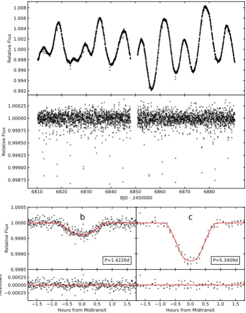
Fig. 1.Upper panel: K2-36 light curve observed by K2, showing the modulation induced by the stellar rotation.Middle plot: K2-36 flattened light curve, with the rotation modulation filtered-out. The observed dim-ming events correspond to the transits of the two planets.Bottom panel: transit light curves for K2-36 b and K2-36 c folded at their best-fit or-bital periods (Table 2). The curves in red are our best-fit transit models, and the residuals are also shown.

cadence K2SFF1_{light curve processed as described by} Vander-burg & Johnson (2014) and VanderVander-burg et al. (2016), and refined by simultaneously fitting for spacecraft systematics, stellar vari-ability, and the planetary transits. The light curve is shown in the upper panel of Fig. 1. A gap is visible between epochs BJD 2 456 848 and 2 456 850.9, during which the observations were interrupted in order to downlink the data. During that time Ke-pler changed orientation, which also changed the heating due to the Sun and introduced an offset in the photometry. The middle panel in Fig. 1 shows the flattened light curve corrected for the modulation due to the stellar rotation, and it is that we used to model the planetary transit signals.

2.2. HARPS-N spectroscopy

We observed K2-36 over three seasons, between the end of Jan-uary 2015 and the end of May 2018, with the high-resolution and stabilised spectrograph HARPS-N (Cosentino et al. 2014) at the Telescopio Nazionale Galileo (TNG) on the island of La Palma. A total of 83 echelle spectra have been secured on fiber A, all with an exposure time of 1800 seconds. Their average signal-to-noise ratio S/N per pixel is 34, as measured at wavelength

λ ∼550 nm. Two of them have S/N<15 (taken at epochs BJD 2 457 810.586681 and 2 457 890.464286), and they have been

discarded from further analysis due to their low quality. Fiber B was used to collect sky spectra. The spectra were reduced with version 3.7 of the HARPS-N Data Reduction Software (DRS).

We performed an analysis to identify the RV measurements potentially contaminated by moonlight. This check is particu-larly necessary for a target such as K2-36, which lies close to the ecliptic plane. The procedure adopted for this analysis is the same as the one described in Section 2.1 of Malavolta et al. (2017a). We have found one potentially contaminated spectrum at epoch BJD 2 457 054.632798, but since our analysis is not conclusive we have decided to include it in the final dataset, which thus consists of 81 spectra.

3. Stellar parameters

Adaptive optics imaging did not detect stellar companions near K2-36 (Sinukoff et al. 2016), and there is no evidence in the cross-correlation function (CCF) of the HARPS-N spectra for more than one component. We derived new values for the funda-mental stellar parameters from the analysis of HARPS-N spectra and using data from theGaiaDR2 catalogue. The atmospheric parameters were first determined separately using three different algorithms.

Equivalent widths. In the classical curve-of-growth ap-proach, we derive temperature Teff and microturbulent velocity

ξtby minimizing the trend of iron abundances (obtained from the equivalent width of each line) with respect to excitation potential and reduced equivalent width, respectively. The surface gravity loggis obtained by imposing the same average abundance from neutral and ionized iron lines. We used ARESv22 _{(Sousa et al.} 2015) to measure the equivalent widths, and usedMOOG3 (Sne-den 1973) jointly with the ATLAS9grid of stellar model atmo-spheres from Castelli & Kurucz (2004) to perform line analy-sis and spectrum syntheanaly-sis, under the assumption of local ther-modynamic equilibrium (LTE). We followed the prescription of Andreasen et al. (2017) and applied the gravity correction from Mortier et al. (2014). The analysis was performed on the result-ing co-addition of individual spectra. We getTeff =4800±59 K, logg=4.73±0.15 (cgs), and [Fe/H]=-0.15±0.03 dex.

Atmospheric Stellar Parameters from Cross-Correlation Functions (CCFpams). This technique is described in Mala-volta et al. (2017b), and the code is publicly available4. We get

Teff = 4841±37 K, logg = 4.60±0.10 (cgs), and [Fe/H]= -0.19±0.04 dex. We report here the internal errors, which are likely underestimated.

Stellar Parameter Classification (SPC). The SPC technique (Buchhave et al. 2012, 2014) was applied to 55 spectra with high S/N, and the weighted average of the individual spectroscopic analyses yielded stellar parameters ofTeff =4862±50 K, logg= 4.57±0.10 (cgs), and [m/H]=-0.05±0.08 dex. For the projected rotational velocity we can reliably impose only the upper limit

vsini?<2 km s−1_.

3.1. The age of K2-36

Inferring the age of this planetary system is relevant for inves-tigating its origin and evolution, but it is a difficult issue for a K dwarf when using only stellar evolution isochrones. Based on the rotational modulation observed in theK2 light curve (Sect.

2_{Available at http://www.astro.up.pt/∼sousasag/ares/} 3_{Available at http://www.as.utexas.edu/∼chris/moog.html} 4_{https://github.com/LucaMalavolta/CCFpams}

5.1) and on a rotation-age relationship (Scott Engle, private com-munication), the age of K2-36 is found to be 1.5±0.4 Gyr, which agrees with our measured average level of chromospheric activ-ityhlogR0_HKi=-4.50 dex.

Using the relation of Mamajek & Hillenbrand (2008) based on gyrochronology (eqs. [12]-[14]), and adopting Prot=16.9±0.2 as the rotation period of K2-36 (Sect. 5.1), we derive an age of 1.09±0.13 Gyr, although the color index of K2-36 (B−V=0.96, corrected for the extinctionE(B−V)=0.03 using the 3D Pan-STARRS 1 dust map of Green et al. 2018) is slightly out the range of validity for that calibration (0.5<B−V<0.9). This result is in agreement with the previous estimate.

We also carried out Galactic population assignment using the classification scheme by Bensby et al. (2003, 2005), the K2-36’s systemic radial velocity from HARPS-N spectra, andGaiaDR2 proper motion and parallax. We obtain a thick disk–to–thin disk probability ratio thick/thin = 0.1, implying that K2-36 is sig-nificantly identified as a thin-disk object, presumably not very old.

Finally, we searched for evidence of the lithium absorption line at 6707.8 Å (Fig. 2). We compared the co-added spectrum with four models, each differing only in the assumed Li abun-dance. The lithium line is not detectable within the noise of the continuum, and we set an upper limit ofA(Li)<0.0. The lithium depletion in K2-36 is comparable to, or lower than, that observed for stars of the same temperature and spectral type in 600-800 Myr-old open clusters with similar metallicity (e.g., Soderblom et al. 1995; Sestito & Randich 2005; Somers & Pinsonneault 2014; Brandt & Huang 2015). We thus set an approximate lower limit for the age of K2-36 att=0.6 Gyr.

3.2. Age-constrained final set of stellar parameters

We used our estimated age of K2-36 to derive a final set of funda-mental stellar parameters, including the stellar mass and radius. To this purpose we have constrained the stellar age to be in the range of 600 Myr to 2 Gyr. The parameters were obtained with the packageisochrone(Morton 2015), following the prescrip-tions of Malavolta et al. (2018). The photospheric parameters of the star obtained with the three different techniques outlined earlier in this Section were used as priors together with the pho-tometric magnitudes V, K, WISE1 and WISE2, and the parallax fromGaia, within a Bayesian framework. The stellar evolution models Dartmouth (Dotter et al. 2008) and MIST (Dotter 2016; Choi et al. 2016; Paxton et al. 2011) were used, thus a total of six different sets of posteriors for the fitted parameters have been derived. The final results are listed in Table 1 and repre-sent the 50th, 15.86thand 84.14th percentiles (the last two used for defining the error bars) after combining all the posteriors to-gether (32310 samples) to take into account the differences ex-isting between the different stellar evolution models. Our model provides an estimate of the extinctionAVat the distance of the star,AV=0.09+₋0₀._.09₀₇ mag. This value is consistent with zero and is in agreement with the results of the 3D dust mapping with Pan-STARRS 1.

4. Photometric transit analysis

6702 6703 6704 6705 6706 6707 6708 6709 6710 6711 Wavelength (Å)

0.5 0.6 0.7 0.8 0.9 1.0

R

el

at

iv

e

fl

ux

Li=1.00 Li=0.50 Li= 0.00 Li=-1.00

6707 6708

Wavelength (Å) 0.88

0.90 0.92 0.94 0.96 0.98 1.00 1.02

R

el

at

iv

e

fl

ux

Li=1.00 Li=0.50 Li= 0.00 Li=-1.00

Fig. 2.Top panel: portion of the HARPS-N co-added spectrum of K2-36 containing the LiI line at 6707.8 Å, compared to four different syntheses (lines of various colors and styles), each differing only for the assumed lithium abundance.Bottom panel: zoom-in view of the region around 6707.8 Åto enable easier comparison between the observed data and model spectra for low Li abundances.”

parameters per planet (time of transit, period,Rp/R?, semi-major axis, and inclination). Our model also assumes zero eccentricity and non-interacting planets. The parameters were estimated

us-ingemcee(Foreman-Mackey et al. 2013), a python package to

perform Markov chain Monte Carlo (MCMC) analysis. Conver-gence was determined by requiring the Gelman-Rubin statistic (Gelman & Rubin 1992) to be less than 1.1 for all parameters. The only difference between our analysis and that of Mayo et al. (2018) is that we included a prior on the stellar density ρ in the light curve model fit. Specifically, at each step in the MCMC simulation we took the stellar density estimated from the transit fit at that step and applied a Gaussian prior to penalize values dis-crepant from our spectroscopic estimate ofρ. Table 2 summa-rizes the fit results. We see that, while our results are consistent with those in Mayo et al. (2018), the prior on the stellar den-sity reduced the uncertainties in planetary radii, inclinations and transit durations. Planet radii are consistent within 1σwith those derived by Sinukoffet al. (2016), and have a similar precision.

Based on their radii, K2-36 b and K2-36 c are each repre-sentative of one of the two planet populations in the radius dis-tribution, below∼1.8R⊕and above∼2R⊕, as characterized by Fulton & Petigura (2018). We note that the mutual inclination between the orbital planes of the planets (∆I ≤3◦_{) is in} agree-ment with the results of Dai et al. (2018) based on the analysis of Kepler/K2 multi-planet systems (not including K2-36). They

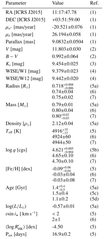
Table 1.Summary of the fundamental stellar parameters of K2-36.

Parameter Value Ref.

RA [ICRS J2015] 11:17:47.78 (1) DEC [ICRS J2015] +03:51:59.00 (1)

µα∗[mas/year] -20.521±0.076 (1) µδ[mas/year] 26.194±0.058 (1) Parallax [mas] 9.0832±0.0504 (1)

V[mag] 11.803±0.030 (2)

B−V 0.992±0.064 (2)

Ks[mag] 9.454±0.025 (3)

WISE/W1 [mag] 9.379±0.023 (4) WISE/W12 [mag] 9.442±0.020 (4) Radius [R] 0.718+−00..008006 (5a)

0.74±0.04 (6) 0.75±0.02 (7) Mass [M] 0.79±0.01 (5a)

0.80±0.04 (6) 0.80+0.02

−0.03 (7)

Density [ρ] 2.12±0.04 (5a)

Teff[K] 4916+−3537 (5)

4924±60 (6) 4944±50 (7) logg[cgs] 4.621+0.005

−0.004 (5b)

4.65±0.10 (6) 4.70±0.10 (7) [Fe/H] [dex] -0.09+0.06

−0.04 (5)

-0.03±0.04 (6) -0.03±0.08 (7) Age [Gyr] 1.4+0.4

−0.5 (5a)

1.5±0.4 (5c) 1.1±0.2 (5d) log(L/L) -0.57±0.01 (5a) vsini?[ km s−1_{] <2 (5)}

2±1 (6)

hlogR0

HKi[dex] -4.50 (5)

Prot[days] 16.9±0.2 (5)

Notes. (1) Gaia DR2 (Gaia Collaboration et al. 2016, 2018); (2) APASS DR9 (Henden et al. 2015); (3) 2MASS Catalog (Skrutskie et al. 2006); (4) WISE Catalog; (5) this work; (5a) this work, derived from isochrones by imposing an age in the range 600 Myr-2 Gyr; (5b) de-rived from isochrones, and not from spectral analysis; (5c) based on a rotation-age relationship, and consistent with the measuredhlogR0

HKi;

(5d) based on the activity-age calibration of Mamajek & Hillenbrand (2008); (6) Sinukoffet al. (2016); (7) Mayo et al. (2018).

found that when the innermost planet is closer to the host star thana/R?=5,∆Ican be likely greater than∼5◦_{, and this effect} could also depend on the orbital period ratio, with pairs with

5. Stellar activity analysis

5.1. Stellar rotation from K2 light curve

Looking at the light curve of K2-36 (Fig. 1, upper panel), the modulation induced by the stellar rotation can be clearly seen. The data before the gap show a two-maxima pattern that repeats every ∼17 days, suggesting that this could be the actual stel-lar rotation period Prot. The scatter of the data before the gap isσphot=2.4%, which increases toσphot=3.9% for data collected after the gap. A positive trend is seen in the second batch of data, that suggests that the active regions on the stellar photosphere are evolving with a timescale comparable with the stellar rotation period. However, we note that the light curve extracted with the alternative pipelineEVEREST(Luger et al. 2016) shows a weaker trend (light curve not shown here), implying that it could be not entirely astrophysical in origin. The highest increase in the rel-ative flux of the light curve maxima is limited to ∼0.2%, and it is observed between the last two rotation cycles. To determine

Protwe computed the autocorrelation function (ACF) of the light curve using the DCF method by Edelson & Krolik (1988) (Fig. 3). The ACF has been explored up to the 80-day time span. The highest ACF peak occurs at∼16.7 days. We modelled this peak with a Gaussian profile5_{in order to determine the error onP}

rot, that we assume to be equal to the Gaussian RMS width. We get

Prot=16.7±1.9 days.

Since the light curve shows evidence for quasi-periodic vari-ations on a timescale of the order ofProt, this makes it interesting to analyse the data using a Gaussian process (GP) regression as done, e.g., by Haywood et al. (2014), Cloutier et al. (2017), or Angus et al. (2018) to model space-based photometry, adopting a quasi-periodic kernel defined by the covariance matrix

K(t,t0)=h2·exp

−(t−t 0₎2

2λ2 −

sin2 π(t−t 0₎

θ !

2w2

+ +σ2

phot,K2(t)·δt,t0 (1)

wheret andt0_{represent two different epochs. The four} hyper-parameters areh, which represents the amplitude of the corre-lations; θ, which parametrizes the rotation period of the star;

w, which describes the level of high-frequency variation within a complete stellar rotation; and λ, which represents the decay timescale of the correlations and can be physically related to the active region lifetimes. The flux error at timet is indicated by

σphot,K2(t), andδt,t0is the Kronecker delta. We introduced a free parameter to model the offset due to the gap in the K2 obser-vations. Since the computing time for a GP regression scales as N3, where N is the number of data points, we analysed the 6-hr binned light curve instead of the full dataset.

All the GP analyses presented in this work (see also Sect. 5.2 and 6) were carried out using the publicly available Monte Carlo sampler and Bayesian inference tool MultiNestv3.10 (e.g. Feroz et al. 2013), through thepyMultiNest wrapper (Buch-ner et al. 2014), by adopting 800 live points and a sampling effi -ciency of 0.5. All the logarithms of the Bayesian evidence (lnZ) mentioned in our work were calculated by MultiNest. The GP component of our code is the publicly availableGEORGEv0.2.1 python module (Ambikasaran et al. 2016). The results of the analysis are summarized in Table 3. The rotation period, that

5_{using LMFIT, a Non-Linear Least-Squares Minimization and}

Curve-Fitting for Python.

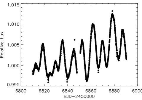
we left free to vary between 0 and 20 days, is consistent with, but more precise than, the ACF estimate (Prot=16.9±0.2 days). The best-fit value for the evolution timescale of the active re-gions is well constrained (λ = 106+₋14₁₁ days) and of the order of a few rotation periods. The best-fit value for the offset is 0.0036±0.0004, and Fig. 4 shows the light curve corrected for the offset. Within the framework of a quasi-periodic model, the corrected light curve shows that the active regions on one hemi-sphere are evolving faster than those on the opposite side of the stellar disk, because the relative height of one maximum has in-creased by∼1.2% over the observation time span.

Using our measure for the stellar radius and the upper limit for vsini? (which coincides with the best-fit value of Sinukoff et al. 2016), the expected maximum rotation period isProt=17.7 days. This result implies that the projected inclination of the spin axis isi?∼90◦.

Since the star is active, we searched for flares in the K2 light curve, without finding any clear evidence of large events.

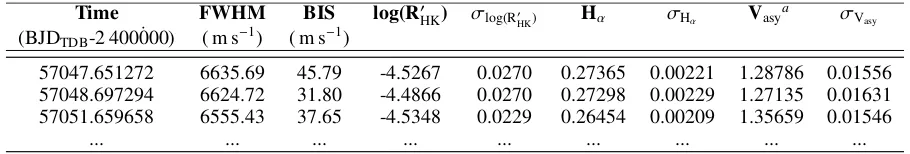
5.2. Stellar activity spectroscopic diagnostics

We characterized the activity of K2-36 during the time span of the HARPS-N observations by analysing a set of standard spec-troscopic indicators. We considered the full width at half maxi-mum (FWHM) of the CCF, the bisector inverse slope (BIS) and Vasy indicators, that quantify the CCF line asymmetry (Vasy is defined by Figueira et al. 2013), the chromospheric activity in-dex log R0_HK, and the activity indicator based on the Hαline (de-rived following the method described in Gomes da Silva et al. 2011). The time series of all the indicators are listed in Table 4 and shown in Fig. 5. Extending to HARPS-N the results by San-terne et al. (2015) valid for the HARPS spectrograph, the uncer-tainties of the FWHM and BIS are fixed to 2σRV, whereσRVare the RV internal errors. Positive trends are clearly visible for the FWHM, log R0_HK, and Hα index, pointing out that the level of activity of K2-36 increased during the time span of our observa-tions. These trends could be part of a long-term activity cycle, but our time span of∼3.5 years is not extended enough to con-firm this. We note that the dispersion in the FWHM, BIS, Vasy and Hαdata increased with time, as a consequence of the increas-ing levels of activity. We calculated the frequency spectrum of these datasets using the Generalised Lomb-Scargle (GLS) algo-rithm (Zechmeister & Kürster 2009), after correcting the trends in the FWHM, logR0_HK, and Hα data by subtracting from each seasonal data chunk the corresponding average value. The peri-odograms are shown in Fig. 5. For the FWHM, BIS, and Vasy we find the highest peak at 8.6 days; for logR0

HKthe peak with the highest power occurs at 16.7 days, and for the Hαindex the

main peak is at 12.9 days, even though peaks of slightly lower power occur atProtand its first harmonic. In conclusion, these indicators appear modulated overProtor Prot/2. We note that a strong correlation exists between logR0

HKand Hα(ρSpear=0.8). We fitted all the indicators with a quasi-periodic GP model, as explained in Sect. 4. Since they have been extracted from the same spectra used to measure the RVs, the outcomes of such analysis are important to eventually set up the analysis of the RVs, in order to properly remove the stellar activity contribution. Results of the GP regression are listed in Table 3.

6. RV analysis

Fig. 3.Autocorrelation function of the K2-36 light curve shown in Fig. 1.

Fig. 4. K2-36 light curve corrected for the offset introduced by the gap in the K2 observations (see Fig. 1 for comparison). An offset of ∼0.36% has been determined through a Gaussian process regression, as described in Section 4.

are not collected during the same seasons. Following Mann et al. (2018), a guess for the RV variability could be estimated as∼

σphot·vsini?, whereσphotis the scatter observed in the K2 light curve. The expected RV variability for K2-36 due to stellar ac-tivity is therefore∼2-5 m s−1_{. According to the calibration for} K-dwarfs derived by Santos et al. (2000), the expected radial velocity scatter for K2-36 is∼9 m s−1_{. We anticipate here that} the signal due to the stellar activity largely dominates the ob-served RVs variations, and it is 5-8 times larger than the semi-amplitudes of the planetary signals, which are of the order of the average RV internal errors (∼2-3 m s−1). When dealing with such an active star it is interesting to compare the results ob-tained from RV extracted with two different procedures, that in principle could be sensitive to stellar activity in different ways for this specific case. Therefore, we have calculated the systemic RVs through the CCF-based recipe of the on-line DRS, using a mask suitable for stars with spectral type K5V, and relative RVs with the TERRA pipeline (Anglada-Escudé & Butler 2012), measured against a high S/N template spectrum. We corrected the TERRA RVs for the perspective acceleration using parallax and proper motion from Gaia DR2. The complete list of RVs

Table 2.Best-fit values obtained from modelling the transit light curve of the K2-36 planets. Data from literature are shown for comparison.

Parameter Best-fit value Reference

Pp,b[days] 1.422614±0.000038 (1)

1.42266±0.00005 (2) 1.422619±0.000039 (3)

T0,b[BJD-2 454 833] 1977.8916±0.0013 (1)

1977.8914±0.0013 (3)

Tdur,b[days] 0.05157+−00..00460034 (1)

Pp,c[days] 5.340888±0.000086 (1)

5.34059±0.00010 (2) 5.340883+0.000088

−0.000089 (3)

T0,c[BJD-2 454 833] 1979.84001±0.00071 (1)

1979.84015+0.00072

−0.00073 (3)

Tdur,c[days] 0.0564+−00..00350027 (1)

Rb/R∗ 0.01828+−00..0007200099 (1)

0.0180+0.0026

−0.0013 (3)

Rc/R∗ 0.04119+0−0..00430029 (1)

0.04+0.17

−0.01 (3)

Rb(R⊕) 1.43±0.08 (1)

1.32±0.09 (2) 1.47+0.22

−0.11 (3)

Rc(R⊕) 3.2±0.3 (1)

2.80+0.43

−0.31 (2)

4.0+14.0

−1.0 (3)

ib[deg] 84.45+−00..7848 (1)

86.3+2.7

−6.2 (3)

ic[deg] 86.917+−00..066056 (1)

85.5+3.9

−3.3 (3)

bb 0.66+−00..0609 (1)

bc 0.89+0−0..0102 (1)

ab[R?] 6.63±0.11 (1)

ab[AU] 0.0223±0.0004 (1)

ac[R?] 16.01+0−0..2627 (1)

ac[AU] 0.054±0.001 (1)

Teq,b[K] 1224±13 (1a)

Teq,c[K] 788±9 (1a)

InsolationSb[S⊕] 529±23 (1)

InsolationSc[S⊕] 90±4 (1)

Notes.(1) This work. (1a) This work, assuming the Bond albedoAb=0.3

(2) Sinukoffet al. (2016). (3) Mayo et al. (2018)

is presented in Table 5. We summarize general properties of the two RV datasets in Table 6, and show the time series in Fig. 6. One common feature is the increase of the scatter observed in the last two seasons with respect to the first. This is a consequence of the increasing stellar activity discussed in Sect. 5.2. The scatter over the time span is similar for all the methods, and the internal errors calculated with TERRA are on average lower than those of the DRS.

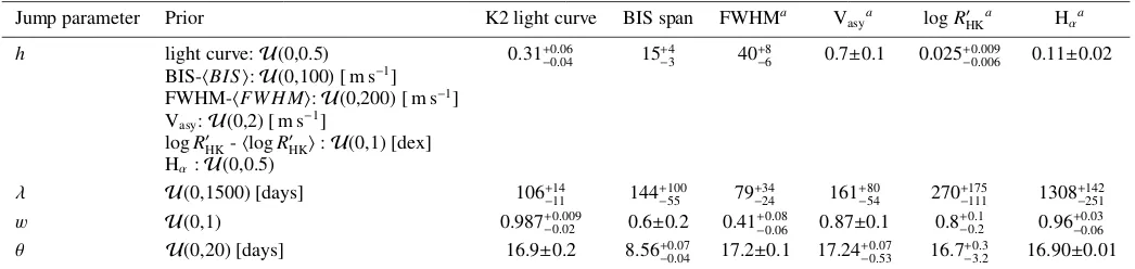
Table 3.GP hyper-parameters of a quasi-periodic model applied to the K2 light curve (6-hr bins), and to the asymmetry and activity index time series derived from HARPS-N spectra. Uncertainties are given as the 16th_{and 84}th_{percentiles of the posterior distributions.}

Jump parameter Prior K2 light curve BIS span FWHMa _V

asya logR0HK

a _H

αa

h light curve:U(0,0.5) 0.31+0.06

−0.04 15+

4

−3 40+

8

−6 0.7±0.1 0.025+ 0.009

−0.006 0.11±0.02

BIS-hBISi:U(0,100) [ m s−1_]

FWHM-hFW H Mi:U(0,200) [ m s−1_]

Vasy:U(0,2) [ m s−1]

logR0

HK-hlogR

0

HKi:U(0,1) [dex]

Hα:U(0,0.5)

λ U(0,1500) [days] 106+14

−11 144+

100

−55 79+

34

−24 161+

80

−54 270+

175

−111 1308+

142

−251

w U(0,1) 0.987+0.009

−0.02 0.6±0.2 0.41+

0.08

−0.06 0.87±0.1 0.8+

0.1

−0.2 0.96+

0.03

−0.06

θ U(0,20) [days] 16.9±0.2 8.56+0.07

−0.04 17.2±0.1 17.24+0

.07

−0.53 16.7+0

.3

−3.2 16.90±0.01 (a)_{Time series not corrected for the long-term trend.}

7000 7500 8000

6600

6700

FWHM [m/s]

0.0

0.2

0.4

0.0

0.1

0.2

0.3

Power, FWHM

7000 7500 8000

0

25

50

75

100

BIS [m/s]

0.0

0.2

0.4

0.0

0.2

0.4

Power, BIS

7000 7500 8000

1.2

1.3

1.4

V

0.0

0.2

0.4

0.0

0.1

0.2

0.3

Po

we

r,

V

7000 7500 8000

Time [BJD - 2450000]

4.6

4.5

4.4

log

R

'

0.0

0.2

0.4

Frequency [cycle/day]

0.00

0.05

0.10

0.15

0.20

Po

we

r,

log

R

'

7000 7500 8000

Time [BJD - 2450000]

0.27

0.28

0.29

H

0.0

0.2

0.4

Frequency [cycle/day]

0.0

0.1

0.2

Po

we

r,

H

0.0 0.2 0.4 0.6 0.8 1.0

Frequency [cycle/day]

0.0 0.2 0.4 0.6 0.8 1.0

Window function

0.02 0.01 0.00 0.01 0.02 0.0

0.5 1.0

Fig. 5.Time series of the FWHM, BIS and VasyCCF line diagnostics, and the log(R0HK) and Hαactivity indexes, shown next to their corresponding

GLS periodograms (after removing the trends in the FWHM, log(R0

HK) and Hαdata as described in the text). The dashed horizontal lines mark

the mean values, to highlight the increasing trend visible in the FWHM, log(R0

HK), and Hαdata. Vertical dotted lines in the periodograms mark

the locations of the stellar rotation period, as derived from K2 photometry, and its first harmonic. The panel in the bottom right corner shows the window function of the data. A zoomed view of the low-frequency part of the spectrum is shown in the inset plot, and a vertical dotted line marks the 1-year orbital frequency of the Earth.

the orbital periods and time of inferior conjunction for K2-36 b and K2-36 c. We assume independent Keplerian motions (i.e. ig-noring mutual planetary perturbations, which would be signifi-cantly below 1 mm s−1) in all the cases and, especially consid-ering the short orbital period of K2-36 b, we did not bin the data on a nightly basis to make use of all the available information in each single data point.

6.1. Frequency content and correlation with activity indicators

resid-uals of the RVs with a GLS periodogram (using DRS data only because of the similarities with the periodogram of the TERRA RVs), after subtracting the best-fit sinusoid, and the periodogram shows the main peak atProt. An additional pre-whitening results in a peak at frequency f ∼0.17 d−1_{, which likely corresponds} to the second harmonic ofProt. This analysis points out that the stellar activity component could be mitigated by a sum of at least three sinusoids with periods Prot,Prot/2 andProt/3. This simple pre-whitening procedure does not allow for the identification of significant power at the orbital planetary frequencies, pointing out that the detection of the two planets using only RVs, without the help from transits and an effective treatment of the stellar ac-tivity contribution, is very complicated. We have folded the RVs of each season taken separately at the period P=8.5 days, and we observe a change in the phase of the signal. This suggests that the stellar activity signal has been evolving on a timescale less than one year, and that a quasi-periodic fit of the stellar com-ponent could be more appropriate than a simple combination of sinusoids.

We checked the correlation between the RVs and the CCF line asymmetry and activity indicators discussed in Sect. 5.2 by calculating the Spearman’s rank correlation coefficients. Results are shown in Fig. 7, where we used the RVs from DRS. Signifi-cant anti-correlation exists just between the DRS RVs and BIS6 (ρSpear =-0.65), which is not surprising since they have simi-lar GLS periodograms. This anti-correlation is expected when the observed RV variations are due mainly to the presence of dark spots on the stellar photosphere, as shown by the light curve modulation (Boisse et al. 2011).

6.2. Joint modelling of planetary and stellar signals (1): sum of sinusoids

Based on the results of the GLS analysis, first we tested a model (hereafter model 1) with the activity component described by a sum of three sinusoids, each with periods sampled around Prot,

Prot/2 andProt/3, using the priors indicated in Table 7. We mod-elled the planetary signals as circular orbits. In total, 17 free pa-rameters were used, including the uncorrelated jitter and offset, that for the DRS RVs corresponds to the systemic velocity. Table 7 shows the results from the analysis of the DRS and TERRA datasets. The semi-amplitude Kb is fitted with a relative error of∼50%, while that of the signal induced by K2-36 c is nearly twiceKb. We note that the required uncorrelated jitterσjitis more than twice the typical internal errorσRV∼2-3 m s−1.

6.3. Joint modelling of planetary and stellar signals (2): de-trending using the BIS line asymmetry indicator

Since a significant anti-correlation is observed between the DRS RVs and the BIS asymmetry indicator, we modelled the stellar signal contribution by including a linear term cBIS·BIS in the model (hereafter model 2). The planetary orbits were fixed to the circular case. For the semi-amplitudes of the planetary sig-nals we get estimates that are nearly twice and nearly half those derived for model 1, for planet b and c respectively:Kb=4.8+₋1₁._.8₇

m s−1_{and K}

c = 2.8+−11..75 m s

−1_{. Since ln}Zmodel 1

Zmodel 2

'+10, which

corresponds to a posterior odds ratio ' 2×104_{:1, this model} is very significantly disfavoured, according to the conventional scale adopted for model selection (see, e.g., Feroz et al. 2011).

6_{Since the BIS span indicator is extracted with the DRS pipeline,}

we limit this analysis to the DRS RVs only.

6.4. Joint modelling of planetary and stellar signals (3): Gaussian process regression analysis

We analysed the RV datasets with a GP regression using the quasi-periodic kernel (Eq. 1) to model the correlated signal in-troduced by the stellar activity contribution. Since both signals modulated onProtandProt/2 are present in the RV timeseries, we left the hyper-parameterθfree to explore uniformly the range be-tween 0 and 20 days. In general, for the hyper-parametersθ,w, andλwe used the same priors as those in Table 3. We included the parameterσjit, which is summed in quadrature withσRVin Eq. 1, to take into account other sources of uncorrelated noise not included inσRV(t).

We first considered the case of circular orbits, then we in-cluded the eccentricitieseb andec as free parameters. The re-sults of the analyses are shown in Table 8. Concerning the circu-lar model, looking at the best-fit values of the hyper-parameters,

θis determined with high precision and its value corresponds to Prot, and the evolutionary timescale of the active regions λ is∼5-8 timesProt, depending on the RV extraction algorithm. This is in very good agreement with the results of the analysis of the light curve and the FWHM activity diagnostic, while there is evidence for a slightly longer evolutionary timescale from the logR0_HK activity index. The Doppler semi-amplitudeKb is in agreement within the errors with that obtained from model 1, both for DRS (Kb=2.1±0.9 m s−1) and TERRA (Kb=2.6±0.7 m s−1_{), but more precise. The mass of K2-36 b is measured with} a significance of ∼ 2.5σ (DRS,mb = 3.2₋+1₁._.4₃ M⊕) and∼3.6σ (TERRA,mb = 3.9±1.1 M⊕), and there is agreement within 1σbetween the two RV extraction pipelines. As for K2-36 c, the mass is measured at best with a significance of∼3.5σ(TERRA,

mc =7.8±2.3 M⊕), and all the values are in agreement within 1σ. When compared to model 1, the semi-amplitude of the K2-36 c signal is lower for both DRS and TERRA, and more precise.

Our analysis does not constrain the eccentricities of the two planets. In fact, for K2-36 b we get eb,DRS = 0.41+₋0₀._.33₃₀ (68.3th _{percentile=0.57) and e}

b,TERRA = 0.51+₋₀0_..26₃₇ (68.3th per-centile=0.65), while for K2-36 c we get ec,DRS = 0.18+−00..2312 (68.3th _{percentile=0.27) and e}

c,TERRA = 0.14+−00..1710 (68.3 th

per-centile=0.21). For both planets, the eccentricity differs from zero with a significance less than 1.5σ, and the peak of the posterior distribution ofecoccurs at zero. Therefore we conclude that our data do not allow us to constrain the eccentricities. Moreover, the eccentric model is statistically disfavoured with respect to the circular model for both the DRS (lnZcircular−lnZecc=+2) and TERRA (lnZ_circular−lnZ_ecc=+2.5) datasets.

Table 6.Properties of the two RV datasets analysed in this work.

Pipeline RMS (all data) RMS (1st_{seas.) RMS (2}nd_{seas.) RMS (3}rd_{seas.) Median internal errorσ} RV

[ m s−1_{] [ m s}−1_{] [ m s}−1_{] [ m s}−1_{] [ m s}−1_]

DRS 14.9 9.8 15.6 15.5 3.1

TERRA 14.7 9.4 14.8 16.2 2.3

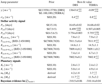
Table 7.Results of the MC analysis performed on the RVs extracted with the DRS and TERRA recipes using a sum of three sinusoids to model the stellar activity component. Uncertainties are given as the 16th_{and 84}th_{percentiles of the posterior distributions.}

Jump parameter Prior Best-fit value

DRS TERRA

γ[ m s−1_{] U(13550,13750) [DRS] 13643.6}+0.8

−0.9 -0.09+ 0.84

−0.86 U(-100,100) [TERRA]

σjit[ m s−1] U(0,20) 6.4−+00..87 6.8+0

.7

−0.6

Stellar activity signal

Prot[days] U(15,18) 16.65±0.02 16.68±0.02

Prot/2 [days] U(7,9.5) 8.499+0−0..006005 8.507±0.005

Prot/3 [days] U(4.5,6.5) 5.754±0.003 5.755+0−0..004138

Kact,P=Prot[ m s

−1_{] U(0,30) 7.8±1.2 7.9±1.2}

T0,act,P=Prot[BJD-2 450 000] U(7800,7820) 7811.5±0,4 7811.9+ 0.5

−0.4

Kact,P=Prot/2[ m s

−1_{] U(0,30) 14.6±1.1 14.5±1.1}

T0,act,P=Prot/2[BJD-2 450 000] U(7800,7810) 7809.4±0.2 7809.1±0.2

Kact,P=Prot/3[ m s

−1_{] U(0,20) 7.4±1.4 6.7±1.3}

T0,act,P=Prot/3[BJD-2 450 000] U(7800,7808) 7802.9±0.2 7802.8+ 0.3

−0.2

Planetary signals

Kb[ m s−1] U(0,10) 2.8±1.3 2.4±1.2

Kc[ m s−1] U(0,10) 5.0±1.4 4.9±1.4

mb[M⊕] derived 4.2±1.8 3.7+−11..87

mc[M⊕] derived 11.7−+33..04 11.5±3.2

Bayesian evidence ln(Z)model 1 -310.5±0.06 -310.14±0.04

6.5. Adopted results

We tested three different models to derive the main planetary pa-rameters. According to their Bayesian evidences the GP quasi-periodic and circular model is strongly favoured over all the other models (in particular lnZmodel 3

Zmodel 1

'+14.5 for the TERRA

dataset, and lnZmodel 3

Zmodel 1

'+9 for the DRS dataset), therefore we adopt this as the best representation for the K2-36 sys-tem based on our data. Since the relative errors on the semi-amplitudes Kb and Kc are lower for the TERRA than for the DRS dataset, we adopt as our final solution the best-fit values obtained with the TERRA RVs. Based on that, K2-36 c has a mass ∼2 times higher than that of K2-36 b (mb=3.9±1.1 M⊕, mc=7.8±2.3 M⊕), but its bulk density is ∼19% that of the in-nermost planet (ρb=7.2+₋2₂._.5₁g cm−3,ρc=1.3+₋0₀._.7₅g cm−3). By using the relationS/S⊕=(L/L)×(AU/a)2, we derived the insolation fluxes Sb=529±23 S⊕ andSc=90±4 S⊕: planet b is∼6 times more irradiated than K2-36 c. The derived planet equilibrium temperatures areTeq,b=1224±13 K andTeq,c=788±9 K.

6.6. Robustness of the derived planet masses

We devised a test to assess how robust our results are. We simu-latedNsim=100 RV time series using the epochs of the HARPS-N spectra as time stamps, and assuming the TERRA dataset and the results of the GP global model to build the mock datasets.

We added two planetary signals (circular orbits) to the quasi-periodic stellar activity signal, with semi-amplitudes Kb=2.6 and Kc=3.4 m s−1. The orbital periods and epochs of inferior conjunction are those derived from K2 light curve. Each mock dataset has been obtained by randomly shifting each point of the exact solution within the error bar, assuming normal dis-tributions centred to zero and with σ = σRV(t). We use this set of simulated data to test our ability to retrieve the injected signals. We analysed the mock RV time series within the same MC framework used to model the original dataset, and for each free parameter we saved the 16th_{, 50}th _{and 84}th _percentiles. Then, we analysed the posterior distributions of theNsimmedian values, and for the planetary Doppler semi-amplitudes we get

Kb=2.7+₋0₀._.4₅andKc=3.4₋+0₀._.8₆ m s−1(16th, 50thand 84thpercentiles). Since these values are in very good agreement with those in-jected, that are equal to those we get form the GP analysis, this suggests that the best-fit values obtained for the original dataset are accurate.

6.7. Sensitivity of the planetary masses to an extended dataset

(dif-7000 7500 8000 Time [BJD - 2450000] 20

0 20

RV DRS, mean subtracted [m/s] 0.0 0.2 0.4 0.6 0.8 1.0 Frequency [d 1_] 0.0

0.2 0.4

Power, DRS

Original data Residuals, P=8.5 d subtracted

7000 7500 8000

Time [BJD - 2450000] 20

0 20

RV TERRA [m/s]

0.0 0.2 0.4 0.6 0.8 1.0 Frequency [d 1_] 0.0

0.2 0.4 0.6

Power, TERRA

Fig. 6.Left column. Radial velocity time series extracted from HARPS-N spectra using the DRS (upper plot) and TERRA (lower plot) pipelines.Right column. GLS periodograms of the RV time series (blue line). Vertical dashed lines mark the location of the highest peak at∼8.5 days and the stellar rotation frequency, for all the datasets. Vertical dot-ted lines in red mark the orbital frequencies of the K2-36 planets. For the DRS dataset only, we show the periodogram of the residuals, after subtracting the signal with period of 8.5 days (gray line), with the main peak located atP∼16.5 days, which corresponds to the stellar rotation period. The window function of the data (not shown) is the same as in Fig. 5.

ferent for each mock dataset) within a 180-day timespan, six months after the end of the third observing season with HARPS-N (for a total of 121 RV measurements per dataset, includ-ing the original data). We assumed a samplinclud-ing characterized by one RV measurement per night, and adopted the GP quasi-periodic best-fit solution to represent the stellar activity term. We used the sample_conditional module in the GEORGE pack-age to draw samples from the predictive conditional distribu-tion (different for each mock dataset) at the randomly selected epochs. Then, we have injected two planetary signals with semi-amplitudesKb=2.6 andKc=3.4 m s−1and circular orbits, using the ephemeris derived from the K2 light curve. The internal er-rorsσRVof the additional RVs have been randomly drawn from a normal distribution centred on the mean of the internal errors of the original RV dataset and withσequal to the RMS of the real arrayσRV. In order to avoid the selection ofσRVvalues that are too optimistic and never obtained for the original dataset, we have simulated only internal errors greater than 1 m s−1_{. This} analysis suggests that, on average, the significance of the re-trieved semi-amplitudes of the planetary signals are expected to increase to 4.4σfor K2-36 b and to 5.6σfor K2-36 c, and the same result is obtained for the planet masses. Concerning the densities, their significance increases to 4σ(ρb) and to 2.6σ(ρc), thus only of a slight amount with respect to the original dataset. Our conclusion is that, under the hypothesis that the structure of the stellar activity signal is preserved several months after the last epoch of the actual observations, a set of 40 additional RVs (which is an affordable amount of measurements to be collected over one season) does not help in improving the precision of the derived planetary parameters enough to significantly improve the theoretical estimates of the planets’ bulk composition based on theoretical models.

13620 13640 13660

0

25

50

75

100

BIS [m/s]

spear = -0.65

13620 13640 13660

6600

6700

FWHM [m/s]

spear = 0.21

13620 13640 13660

1.2

1.3

1.4

V

spear = 0.35

13620 13640 13660

RV DRS [m/s]

4.6

4.5

4.4

log

(R

0 HK

)

spear = 0.21

13620 13640 13660

RV DRS [m/s]

0.27

0.28

0.29

H

spear = 0.22

Fig. 7.Correlations between radial velocities (from DRS), the CCF line profile indicators, and activity diagnostics.

Fig. 8.Doppler signals due to the K2-36 planets (TERRA radial veloc-ity dataset, after removing the GP quasi-periodic stellar activveloc-ity term), folded according to their transit ephemeris (phase=0 corresponds to the time of inferior conjunction). The histograms show the distribution of the RV measurements along the planetary orbits.

7. Discussion

Table 8.Best-fit solutions for the model tested in this work (quasi-periodic GP model) applied to the HARPS-N RV time series extracted with the DRS and TERRA pipelines. Our global model includes two orbital equations (circular and eccentric case). Uncertainties are given as the 16th_and

84th_{percentiles of the posterior distributions.}

Jump parameter Prior Best-fit value

DRS TERRA

Stellar activity GP model

h[ms−1_{] U(0,30) 16.3}+3.8

−2.7 17.11+ 3.9

−2.8

λ[days] U(0,1500) 131+55

−35 93+

22

−20

w U(0,1) 0.33+0.06

−0.05 0.33±0.05

θ[days] U(0,20) 16.99+0.09

−0.07 17.06±0.08

σjit[ms−1] U(0,20) 2.5±1.0 1.6+−00..89

γ[ms−1_{] U(13550,13750) 13640.7}+4.9

−5.2 -1.7+

5.1

−5.2

Kb[ms−1] U(0,10) 2.1±0.9 2.6±0.7

Kc[ms−1] U(0,10) 2.9±1.1 3.4±1.0

Derived quantities(a)

mb(M⊕) 3.2+1−1..43 3.9±1.1

mc(M⊕) 6.7+2−2..76 7.8±2.3

ρb[gcm−3] 5.9−+22..95 7.2+2

.5

−2.1

ρc[gcm−3] 1.1−+00..65 1.3+0

.7

−0.5

Bayesian EvidencelnZmodel 3 -301.45±0.02 -295.5±0.08

Notes.(a)_{Derived quantities from the posterior distributions. We used the following equations (assumingM}

s+mp Ms):mpsini(Kp·M 2 3 s · √

1−e2_·P13 p)/(2πG)

1

3;a[(M_s·G)13 ·P

2 3 p]/(2π)

2

3, whereGis the gravitational constant. We sete=0 for circular orbits.

Fig. 9. Stellar activity component in the radial velocities (TERRA dataset) as fitted using a GP quasi-periodic model (circular case). Each panel shows one of the three observing seasons. The blue line represents the best-fit solution, and the grey area the 1σconfidence interval.

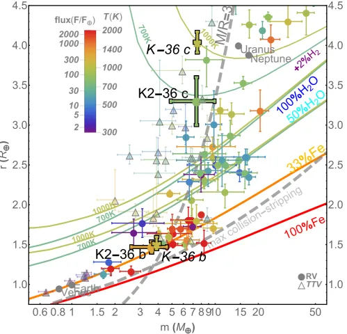
7.1. Planets in the mass-radius diagram

The exoplanet mass-radius diagram is shown in Fig. 11, and it includes the masses of the K2-36 planets derived from the GP analysis of the TERRA dataset. K2-36 b is nicely located on the theoretical curve for planets with Earth-like rocky composition, while the Neptune/sub-Neptune size K2-36 c has a bulk structure compatible with having a H2-dominated gas envelope of∼1−2%

Fig. 10.K2 light curve (upper plot) and stellar activity component in the radial velocities (lower plot; TERRA data for the last two seasons. DRS data show a similar behaviour), folded at the stellar rotation period. The reference epoch corresponding to phase=0 is the same for both datasets. Light curve goes from May, 30th_{to Aug, 21}th_{2014 (K2 campaign C1).}

Spectroscopic data are distinguished according the observing season: black dots are used for data collected in 2017, red dots for those of 2018.

having 1-2% primordial H2/He-dominated envelope at its cor-responding equilibrium temperature (Fig. 12), or an even less massive H2/He envelope if it has not cooled offfrom formation yet. Note the mass of K2-36 c is also less than 10M⊕, the critical core mass required for run-away gas accretion (Rafikov 2006). This may explain why it did not acquire more gas and evolve into a gas giant.

Both methane CH4 and ammonia NH3 (Levi et al. 2013, 2014, 2017), and even H2itself (Soubiran & Militzer 2015), can be incorporated into the H2O-reservoir during the initial forma-tion stage, then out-gassed gradually to replenish a primary en-velope, or form a secondary enen-velope, making K2-36 c a pos-sible example of water-world (Zeng et al. subm.). It is pospos-sible that K2-36 b formed inside the snowline of the system (located at∼1.2 AU, see e.g. Mulders et al. 2015), and K2-36 c formed farther away beyond the snowline, building up a water-rich core and acquiring almost twice the mass of planet b. In fact, it is expected from cosmic element abundance that just beyond the snowline there is about equal mass available in solids from icy material (including methane clathrates and ammonia hydrates, which both contain H2O) and from rocky material (including primarily Mg-silicates and (Fe,Ni)-metal-alloy), for planet to ac-crete from, while only rocky material would remain available in solids inside the snowline (Lewis 1972, 2004).

7.2. Comparing K2-36 to Kepler-36

An interesting comparison can be made between the K2-36 and Kepler-36 planetary systems. The two-planet system Kepler-36 was discussed by Carter et al. (2012), and then studied by Lopez & Fortney (2013), Quillen et al. (2013), Owen & Morton (2016), Bodenheimer et al. (2018). Kepler-36 is a 6.8 Gyr moderately-evolved Sun-like star, thus older than K2-36 and with very simi-lar metallicity ([Fe/H]=-0.20±0.6). Both Kepler-36 planets have very similar masses and radii compared to the corresponding K2-36 planets (see Fig. 11. The innermost planets b are con-sistent with Earth-like rocky composition (see Fig. 11). Kepler-36 c has a larger radius than that of K2-Kepler-36 c, by adopting the more recent estimate of Fulton & Petigura (2018)7, and lower density. Kepler-36 planets have different densities and close or-bits with periods near the 7:6 mean motion resonance. They both receive nearly half the insolation of K2-36 b, and have insolation difference much lower than that for K2-36 planets ([Sb−Sc]Kep−36 ∼45S⊕, and [Sb−Sc]K2−36 ∼440S⊕). They are both susceptible to H2-He atmospheric escape considering their escape velocities and current equilibrium temperaturesTeq≥900 K. According to their measured densities, Kepler-36 b has lost any H2-He gaseous envelope, while planet c still appears inflated and consistent with retaining an envelope of H2/He with some percent in mass at the corresponding insolation. The near 7:6 mean motion resonance indicates that they have reached a sta-ble orbital configuration. If photo evaporation has been driving atmospheric loss, its effects could have been steeply accelerated when the host star moved to the MS turn-offpoint, and it is still eroding the atmosphere of planet c. K2-36 and Kepler-36 planets could have formed in a similar environment, as suggested by the similar host star metallicity, and experienced a similar migration pathway.

7_{also Berger et al. (2018) provided a revised estimate for the radius}

of Kepler-36 c,R=3.689+0.165

−0.153, which is actually very similar to that of

Carter et al. (2012). By adopting this value instead of that from Fulton & Petigura (2018), Kepler-36 c and K2-36 c have their radii compatible within one sigma.

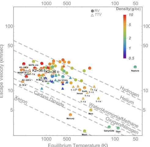
7.3. Comparing K2-36 to WASP-107

Another interesting comparison is with WASP-107, a one-planet system characterized by a 0.9Rjupplanet with a sub-Saturn mass, and with an orbital period very similar to that of K2-36 c (5.7 days), transiting a magnetic active K6V star with rotation period very similar to that of K2-36 (Anderson et al. 2017; Moˇcnik et al. 2017). Transmission spectroscopy has recently enabled the de-tection of helium in a likely extended atmosphere of the planet, for which an erosion rate of 0.1-4% of the total mass per bil-lion years has been calculated (Spake et al. 2018). WASP-107 b has an escape velocity (≥20 km s−1, ormp/Rp ∼3.6) and a sur-face equilibrium temperature (Teq ∼740 K) not very dissimilar to those of K2-36 c. If the sub-Neptune K2-36 c has H2/He as components in its atmosphere, they could currently be escaping at a strong rate, despite intermediate-sized planets (2-4R⊕) pre-sumably having much less H2/He volatiles than WASP-107 b, which would then be depleted faster. Based on this planet-to-planet comparison, K2-36 c may be considered suitable for fu-ture observations to search for evaporating helium. In fact, by assuming an atmosphere composed of 50% H2and 50 %He, and the mass and radius estimated above for K2-36c, the atmospheric transmission spectrum signal of the planet can reach values up to about 160 ppm at five scale heights if it has a clear atmosphere. If the planet has a pure He atmosphere that extend 10 scale heights, it might present He absorption with an amplitude of 500 ppm.

8. Conclusions

We presented a characterization study of the K2-36 planetary system based on data collected with the HARPS-N spectrograph. According to their size, the planets K2-36 b and K2-36 c are lo-cated above and below the photo-evaporation valley, and their derived bulk densities (ρb=7.2+₋2₂._.5₁g cm−3,ρc=1.3+₋0₀._.7₅g cm−3) in-dicate that K2-36 b has an Earth-like rocky composition, while the Neptune/sub-Neptune size K2-36 c is likely surrounded by a significant gas envelope, not yet evaporated. K2-36 is an ideal laboratory to study the role of the photo-evaporation on the evo-lution of low-mass, close-in planets, especially for a relatively young (∼1 Gyr) system, as we determined in this work, with the host star having high levels of magnetic activity.

Acknowledgements. We acknowledge the two anonymous referees for useful

Galileo Galilei of the INAF (Istituto Nazionale di Astrofisica) at the Spanish Observatorio del Roque de los Muchachos of the Instituto de Astrofisica de Ca-narias. This paper includes data collected by the K2 mission. Funding for the K2 mission is provided by the NASA Science Mission directorate. Some of the data presented in this paper were obtained from the Mikulski Archive for Space Telescopes (MAST). STScI is operated by the Association of Universi-ties for Research in Astronomy, Inc., under NASA contract NAS5-26555. Sup-port for MAST for non-HST data is provided by the NASA Office of Space Science via grant NNX13AC07G and by other grants and contracts. This re-search has also made use of data products from the Wide-field Infrared Survey Explorer, which is a joint project of the University of California, Los Ange-les, and the Jet Propulsion Laboratory/California Institute of Technology, funded by the National Aeronautics and Space Administration; of data from the Eu-ropean Space Agency (ESA) missionGaia(https://www.cosmos.esa.int/gaia), processed by the Gaia Data Processing and Analysis Consortium (DPAC, https://www.cosmos.esa.int/web/gaia/dpac/consortium). Funding for the DPAC has been provided by national institutions, in particular the institutions partici-pating in the Gaia Multilateral Agreement.

References

Ambikasaran, S., Foreman-Mackey, D., Greengard, L., Hogg, D. W., & O’Neil, M. 2016, IEEE Trans. Pattern Anal. Mach. Intell., 38, 252

Anderson, D. R., Collier Cameron, A., Delrez, L., et al. 2017, A&A, 604, A110 Andreasen, D. T., Sousa, S. G., Tsantaki, M., et al. 2017, A&A, 600, A69 Anglada-Escudé, G. & Butler, R. P. 2012, The Astrophysical Journal Supplement

Series, 200, 15

Angus, R., Morton, T., Aigrain, S., Foreman-Mackey, D., & Rajpaul, V. 2018, Monthly Notices of the Royal Astronomical Society, 474, 2094

Bensby, T., Feltzing, S., & Lundström, I. 2003, A&A, 410, 527 Bensby, T., Feltzing, S., Lundström, I., & Ilyin, I. 2005, A&A, 433, 185 Berger, T. A., Huber, D., Gaidos, E., & van Saders, J. L. 2018, ApJ, 866, 99 Bodenheimer, P., Stevenson, D. J., Lissauer, J. J., & D’Angelo, G. 2018, ApJ,

868, 138

Boisse, I., Bouchy, F., Hébrard, G., et al. 2011, A&A, 528, A4 Brandt, T. D. & Huang, C. X. 2015, The Astrophysical Journal, 807, 24 Buchhave, L. A., Bizzarro, M., Latham, D. W., et al. 2014, Nature, 509, 593 Buchhave, L. A., Latham, D. W., Johansen, A., et al. 2012, Nature, 486, 375 Buchner, J., Georgakakis, A., Nandra, K., et al. 2014, A&A, 564, A125 Carter, J. A., Agol, E., Chaplin, W. J., et al. 2012, Science, 337, 556

Castelli, F. & Kurucz, R. L. 2004, ArXiv Astrophysics e-prints [astro-ph/0405087]

Choi, J., Dotter, A., Conroy, C., et al. 2016, ApJ, 823, 102

Cloutier, R., Astudillo-Defru, N., Doyon, R., et al. 2017, A&A, 608, A35 Cosentino, R., Lovis, C., Pepe, F., et al. 2014, in Proc. SPIE, Vol. 9147,

Ground-based and Airborne Instrumentation for Astronomy V, 91478C Dai, F., Masuda, K., & Winn, J. N. 2018, ApJ, 864, L38 Dotter, A. 2016, ApJS, 222, 8

Dotter, A., Chaboyer, B., Jevremovi´c, D., et al. 2008, ApJS, 178, 89 Edelson, R. A. & Krolik, J. H. 1988, ApJ, 333, 646

Feroz, F., Balan, S. T., & Hobson, M. P. 2011, Monthly Notices of the Royal Astronomical Society, 415, 3462

Feroz, F., Hobson, M. P., Cameron, E., & Pettitt, A. N. 2013, ArXiv e-prints [arXiv:1306.2144]

Figueira, P., Santos, N. C., Pepe, F., Lovis, C., & Nardetto, N. 2013, A&A, 557, A93

Foreman-Mackey, D., Hogg, D. W., Lang, D., & Goodman, J. 2013, PASP, 125, 306

Fulton, B. J. & Petigura, E. A. 2018, AJ, 156, 264

Fulton, B. J., Petigura, E. A., Howard, A. W., et al. 2017, AJ, 154, 109 Gaia Collaboration, Brown, A. G. A., Vallenari, A., et al. 2018, A&A, 616, A1 Gaia Collaboration, Prusti, T., de Bruijne, J. H. J., et al. 2016, A&A, 595, A1 Gelman, A. & Rubin, D. B. 1992, Statistical Science, 7, 457

Gomes da Silva, J., Santos, N. C., Bonfils, X., et al. 2011, A&A, 534, A30 Green, G. M., Schlafly, E. F., Finkbeiner, D., et al. 2018, MNRAS, 478, 651 Haywood, R. D., Collier Cameron, A., Queloz, D., et al. 2014, MNRAS, 443,

2517

Henden, A. A., Levine, S., Terrell, D., & Welch, D. L. 2015, in American Astro-nomical Society Meeting Abstracts, Vol. 225, American AstroAstro-nomical Soci-ety Meeting Abstracts, 336.16

Levi, A., Kenyon, S. J., Podolak, M., & Prialnik, D. 2017, ApJ, 839, 111 Levi, A., Sasselov, D., & Podolak, M. 2013, ApJ, 769, 29

Levi, A., Sasselov, D., & Podolak, M. 2014, ApJ, 792, 125

Lewis, J. 2004, Physics and Chemistry of the Solar System, International Geo-physics (Elsevier Science)

Lewis, J. S. 1972, Icarus, 16, 241

Lopez, E. D. & Fortney, J. J. 2013, ApJ, 776, 2 Luger, R., Agol, E., Kruse, E., et al. 2016, AJ, 152, 100

Malavolta, L., Borsato, L., Granata, V., et al. 2017a, AJ, 153, 224

Malavolta, L., Lovis, C., Pepe, F., Sneden, C., & Udry, S. 2017b, MNRAS, 469, 3965

Malavolta, L., Mayo, A. W., Louden, T., et al. 2018, AJ, 155, 107 Mamajek, E. E. & Hillenbrand, L. A. 2008, ApJ, 687, 1264

Mann, A. W., Vanderburg, A., Rizzuto, A. C., et al. 2018, The Astronomical Journal, 155, 4

Marcus, R. A., Stewart, S. T., Sasselov, D., & Hernquist, L. 2009, The Astro-physical Journal Letters, 700, L118

Mayo, A. W., Vanderburg, A., Latham, D. W., et al. 2018, AJ, 155, 136 Mortier, A., Sousa, S. G., Adibekyan, V. Z., Brandão, I. M., & Santos, N. C.

2014, A&A, 572, A95

Morton, T. D. 2015, isochrones: Stellar model grid package, Astrophysics Source Code Library

Moˇcnik, T., Hellier, C., Anderson, D. R., Clark, B. J. M., & Southworth, J. 2017, MNRAS, 469, 1622

Mulders, G. D., Ciesla, F. J., Min, M., & Pascucci, I. 2015, The Astrophysical Journal, 807, 9

Owen, J. E. & Morton, T. D. 2016, ApJ, 819, L10 Owen, J. E. & Wu, Y. 2013, ApJ, 775, 105 Owen, J. E. & Wu, Y. 2017, ApJ, 847, 29

Paxton, B., Bildsten, L., Dotter, A., et al. 2011, ApJS, 192, 3

Quillen, A. C., Bodman, E., & Moore, A. 2013, Monthly Notices of the Royal Astronomical Society, 435, 2256

Rafikov, R. R. 2006, ApJ, 648, 666

Santerne, A., Díaz, R. F., Almenara, J.-M., et al. 2015, MNRAS, 451, 2337 Santos, N. C., Mayor, M., Naef, D., et al. 2000, A&A, 361, 265

Sestito, P. & Randich, S. 2005, A&A, 442, 615

Sinukoff, E., Howard, A. W., Petigura, E. A., et al. 2016, ApJ, 827, 78 Skrutskie, M. F., Cutri, R. M., Stiening, R., et al. 2006, AJ, 131, 1163 Sneden, C. 1973, ApJ, 184, 839

Soderblom, D. R., Jones, B. F., Stauffer, J. R., & Chaboyer, B. 1995, AJ, 110, 729

Somers, G. & Pinsonneault, M. H. 2014, ApJ, 790, 72 Soubiran, F. & Militzer, B. 2015, ApJ, 806, 228

Sousa, S. G., Santos, N. C., Adibekyan, V., Delgado-Mena, E., & Israelian, G. 2015, A&A, 577, A67

Spake, J. J., Sing, D. K., Evans, T. M., et al. 2018, Nature, 557, 68

Van Eylen, V., Agentoft, C., Lundkvist, M. S., et al. 2018, MNRAS, 479, 4786 Vanderburg, A. & Johnson, J. A. 2014, PASP, 126, 948

Vanderburg, A., Latham, D. W., Buchhave, L. A., et al. 2016, ApJS, 222, 14 Zechmeister, M. & Kürster, M. 2009, A&A, 496, 577

Zeng, L., Jacobsen, S. B., Hyung, E., et al. 2017, in Lunar and Planetary Science Conference, Vol. 48, Lunar and Planetary Science Conference, 1576 Zeng, L., Jacobsen, S. B., & Sasselov, D. D. 2017b, Research Notes of the AAS,