Mining Interesting Patterns and Rules
in a Time-evolving Graph
Yuuki Miyoshi
∗, Tomonobu Ozaki
†, and Takenao Ohkawa
‡Abstract—Time-evolving graphs, i.e. dynamic networks changing their structures with time, are becoming ubiquitous recently. A typical example is an email communication network whose vertex corresponds to an individual and whose edge corresponds to an email communication within a time period. For the effective analysis of such time-evolving graphs, it must be important to utilize representative local structures in networks as well as time information on edge formation simultaneously.
In this paper, we consider a problem of mining frequent pat-terns and valid rules representing graph evolutions or structural changes in a network with time information. In addition to an effective mechanism for extracting representative patterns and rules, we devise graph-based summarization of discovered rules. By using certain measures provided by the summary, we can expect to find more interesting information that are difficult to obtain in the traditional support and confidence framework. The effectiveness of the proposed framework was confirmed by preliminary experiments using real world email data.
Index Terms—frequent pattern mining, graph mining, graph evolution rule
I. INTRODUCTION
Recently, the study of human activities on social and communication networks attract a large amount of attention. In general, patterns on local structures in those networks can provide useful insight for understanding human activities. Furthermore, because a network changes its structure dynam-ically with time, taking account of temporal information on edge formation will help precise analysis. In this paper, we consider the problem of mining frequent patterns and valid rules that represents graph evolutions, i.e. structural changes in a network with time information.
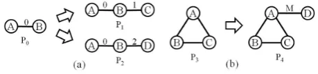
Two types of graph evolutions are discussed. One is an evolution by temporal aspect, and the other is by the surrounding situation. These evolutions are explained with a simple example shown in Fig. 1. In this figure, we assume that each vertex corresponds to a person and each edge represents a communication between persons. The num-ber associated to an edge represents a time period when the communication is conducted. In Fig. 1(a), P1 and P2
represent two graph evolutions with different time periods after the communication between A and B. The order and timing of communications contained inP1 andP2will give
useful insight to understand the evolutions. On the other hands, Fig. 1(b) represents an evolution influenced by the surrounding situation. P4 states that a triangle (P3) causes
an communication between A and D while we do not care
∗Graduate School of Engineering, Kobe University, 1-1 Rokkodai, Nada,
Kobe 657-8501, Japan. Email: [email protected]
†Cybermedia Center, Osaka University, 1-32 Machikaneyama, Toyonaka,
Osaka 560-0043, Japan. Email: [email protected]
‡Graduate School of System Informatics, Kobe University, 1-1 Rokkodai,
[image:1.595.311.541.177.231.2]Nada, Kobe 657-8501, Japan. Email: [email protected]
Fig. 1. two types of graph evolutions
how the triangle is constructed. This kind of information must be useful to understand what structure acts as a trigger for graph evolutions.
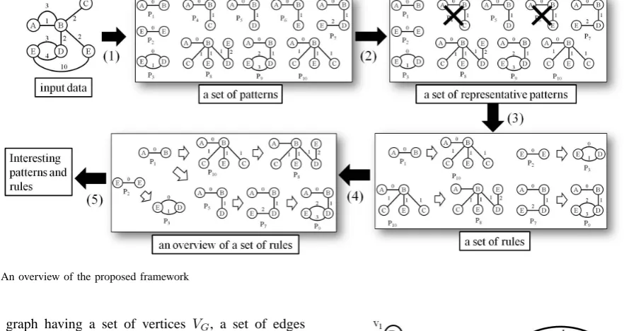
Previous researches on graph pattern discovery have draw-back on analyzing graph evolutions. First, other than a few exceptions, most graph miners can not handle time infor-mation directly. Second, due to a huge amount of extracted patterns and rules, it is difficult to determine important and significant ones. To overcome these difficulties, in this paper, we propose a framework for discovering interesting patterns and rules on graph evolutions. The proposed approach is summarized in Fig. 2. We first mine frequent patterns with a time information ((1) in Fig. 2). Frequent pattern miners often discover a huge amount of patterns. In order to com-press a set of frequent patterns into a representative set, we adopt a structural representative approach proposed in [4] ((2) in Fig. 2). Then, the rules focused on the evolutions will be generated from the obtained patterns ((3) in Fig. 2). We devise two graph-based summarizations of a set of rules to help to discover interesting and important patterns ((4) in Fig. 2). Finally, by investigating these summarizations, we extract characteristic patterns and chains of rules based on some network-based importance measure such as degree centrality ((5) in Fig. 2). The aim of employing network-based measure is to find interesting patterns which are difficult to discover in the standard framework based on support and confidence.
The rest of this paper is organized as follows. In section II, basic notations and definition will be introduced. In section III, our framework for discovering patterns and rules in time-evolving graphs will be explained in detail. Preliminary ex-perimental results are reported in section IV. After describing related work in section V, finally we conclude this paper in section VI.
II. NOTATIONS ANDDEFINITIONS
According to the previous studies[1], [4], [3], we give formal notations and definitions on graphs, patterns and rules with time information.
A. Patterns and Rules in a Time-evolving Graph
Fig. 2. An overview of the proposed framework
labeled graph having a set of vertices VG, a set of edges EG ⊆ VG×VG, a labeling function lG : VG ∪EG → L that maps each element of a graph to an alphabet inL, and a time-stamp function tG : EG → T that assigns a time-point inT to each edge. While multi-edges having different time-stamps are allowed in a time-evolving graph, we assume that labels of vertices and edges never change with time for the simplicity. A graph “input data” in Fig. 2 is an example of time-evolving graphs. In the graph, there are two edges between vertices A and B. One has “1” of time-stamp, the other has “3”.
As a pattern in a time-evolving graph, we employ a
relative time pattern which is a connected time-evolving
graphP = (VP, EP, lP, tP)whose lowest time-stamp is zero (mine∈Eptp(e) = 0). The concept of relative time pattern
is originally introduced in [1]. In this paper, we extend the original definition to allow multi-edges among vertices to represent plural relations and repeated communications in different time-points. Note that, time-points associated to edges in relative time patterns represent the relative relation among the periods of edge formations. For example, a relative time patternP4in Fig. 2 states that an edge between
two vertices B and C is generated in the next period when an edge between A and B is established. Hereafter, we call relative time pattern as time pattern for the sake of simplicity.
We introduce a subgraph relation and support value on time-evolving graphs. A time-evolving graph P1 is said to
be a subgraph of another time-evolving graph P2, denoted
as P1 ⊂ P2, if there exists a parameter ∆ ∈ R and
an injective function f : VP1 → VP2 which satisfies
the conditions: (i) ∀v ∈ VP1[lP1(v) = lP2(f(v)) ], (ii)
∀(u, v) ∈ EP1[lP1(u, v) = lP2(f(u), f(v)) ], and (iii)
∀(u, v) ∈ EP1[tP2((f(u), f(v))) = tP1((u, v)) + ∆]. An
occurrence ofP1inP2with respect to a functionf satisfying
the conditions on subgraph relation is defined as a list o = [v1, v2,· · ·, v|VP1|](vi ∈ VP2, vi =f(ui), ui ∈ VP1)of
vertices inP2mapped from vertices inP1byf. The notation
o(vi) is used to represent thei-th element in an occurrence o. All occurrences of P1 in P2 is denoted as ΦPP12. Fig. 3
shows an example of a set of occurrences of P in G(ΦPG) and their parameter ∆. A listo1 consists of three vertices
Fig. 3. Occurrences of a time patternP in a time-evolving graphG
v3,v2andv1 inGwhich correspond tov0, v1 andv2inP,
respectively.
The support value of a time pattern P in a time-evolving graph G is defined as supG(P) = minvi∈VP{o(vi)|o∈Φ
P
G}/|VG|, i.e. the ratio of minimum number of unique vertices o(vi) in o ∈ ΦPG to the total number of vertices. This definition is a simple adoption of the support value of a pattern in a single graph setting[3]. In Fig. 3,|o(v0)|is the minimum number and the support value
ofP inGis calculated assupG(P) = 0.4. Given a threshold σ, a time patternP is said to be frequent ifsupG(P)≥σ holds.
Then, we consider rules between two time patterns for representing graph evolutions. We adopt graph evolution
rules[1] in the form of Pb → Ph where Pb and Ph are time patterns and Pb is obtained by deleting all the edges having the last or maximal time-point from Ph. The formal definition is given below. For two time patterns Ph and Pb, a rule Pb → Ph is defined as a graph evolution rule with respect to Ph if the following conditions hold: (i)EPb = {e ∈ EPh|tPh(e) < maxe′∈EPh(tph(e′))},
(ii)VPb = {v ∈ VPh|deg(v, EPb) >0} where deg(v, EPb)
denotes the degree ofv inPb, and (iii)Pb is connected. While every time patternPh can not form a graph evolu-tion rulePb →Ph, Ph determines its bodyPb uniquely if suchPbexists. A notationr(Ph)is used to represent a unique rulePb→Phobtained byPh. A rule ofr(P7) =P5→P7in
[image:2.595.76.521.63.297.2]that, if a graph pattern having two edges is established by adding edges A–B and B–D in this order, then an additional edge between D and E will be generated in the next period with a certain probability.
The probability or confidence of a graph evolution rules is discussed below. While two definitions on the strength of graph evolution rules are employed in the previous study[1], we propose another definition of confidence of a graph evolution rule Pb → Ph based on the occurrences of Pb. The confidence value of a graph evolution rule Pb → Ph is defined as confG(Pb → Ph) = |OPb(Ph)|/|Φ
Pb G| where OPb(Ph) denotes a set of occurrenceob ∈ Φ
Pb
G which can be extendable to an occurrence oh ∈ ΦPGh. It is natural to consider that an occurrence of Pb grows into an occurrence ofPhby evolutions. Thus, we believe that this definition, i.e. the ratio of occurrences in Pb grown into an occurrence in Ph, is suitable for capturing the strength of graph evolution rules. Given a threshold τ, a graph evolution rulePb→Ph is said to be valid ifconfG(Pb→Ph)≥τ.
B. Representative Time Patterns
Frequent pattern miners often discover a huge amount of patterns[8]. In order to compress a set of frequent time patterns into a representative set of manageable size, we apply a structural representative approach proposed in [4] which considers two aspects, (i)structural representability and (ii)support preservation. This approach is originally proposed for patterns in a graph database (a set of graphs) without time-stamps, we extend it to handle relative time patterns in a time-evolving graph.
The structural representability is discussed first. Intuitively speaking, the structural difference between two time patterns having the same vertex sets is measured as a degree of differ-ence between edge sets. Given an error tolerance parameter δ, the structural difference between two time patternsP′and P is defined as follows:
dif f(P′, P) = {
min f∈F(P′,P)
d(P′, P, f) (F(P′, P)̸=∅)
∞ (otherwise)
whereF(P′, P)denotes a set of bijective mappings satisfy-ing (i)∀v′ ∈VP′[lP′(v′) =lP(f(v′))]and (ii)d(P′, P, f) =
∑
v′1,v2′∈VP′|I
P′(v′
1, v′2)−IP(f(v′1), f(v′2))| ≤ δ in which
IP(u, v) is an indicator function such that IP(u, v) = 1 if (u, v) ∈ Ep and IP(u, v) = 0 otherwise. We define the structure representable by using the structural difference. A time pattern P′ is said to be structure representable by another time pattern P if an inequality
Rs(P′, P) = min |VP′|=|VP′′|,P′′⊆induce
0 P
dif f(P′, P′′)≤δ
holds where ⊆induce0 denotes an induced subgraph
relationship[4]. In simple words,P′is structure representable byP ifP has a subgraphP′′which shares the same vertex set and similar edge set with P′.
Then, on specifying the degree of support preservation,
smoothed support for time pattern is proposed by slightly
modifying the original definition in [4]. Given a set of fre-quent time patterns T P ={P1,· · ·, Pn} in a time-evolving
graph G, the smoothed supporting occurrence set of Pi is defined asSPi =
∪
Pj∈T P,dif f(Pi,Pj)≤δΦ PJ
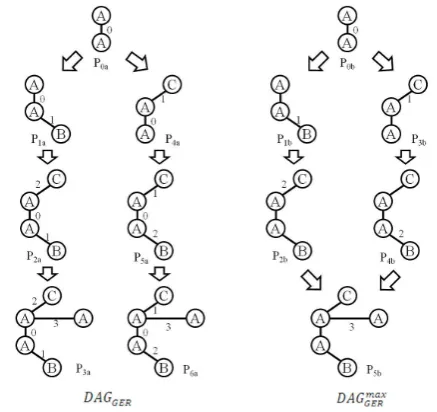
[image:3.595.315.534.52.258.2]G .In other words,
Fig. 4. An example ofDAGGERandDAGmaxGER
SPicontains all the occurrences in structural similar patterns
Pj withPi. Then, the smoothing support value ofPi∈T P is defined as ssupG(Pi) = min1≤i≤|VPi||{o(i)|o ∈ SPi}|.
By using smoothing support, we define the preservation of support value. Given a tolerance parameterϵ, we say that the support of a patternP′ is preserved by another patternP, if an inequality
P s(P′, P) = |ssupG(P)−ssupG(P ′)|
max{ssupG(P), ssupG(P′)} ≤ϵ
holds.
Given two parameters δ andϵ, a time pattern Pi will be judge as representative in a set of frequent time patterns T P ={P1,· · ·, Pn} if a set
CT Pδ,ϵ(Pi) ={Pj ∈T P |Rs(Pj, Pi)≤δ, P s(Pj, Pi)≤ϵ}
is large enough. A concrete algorithm for determining rep-resentative time patterns will be introduced in section III.
C. Graph Evolution DAGs
Compared with the examination of individual graph evolu-tion rule one by one, consideraevolu-tion of a set of graph evoluevolu-tion rules all at once must be effective for finding interesting and important patterns related to graph evolution. For this purpose, we consider a graph-based summarization of a set of graph evolution rules.
Given a set of graph evolution rules GER, a graph
evolution DAG onGER, denoted as DAGGER, is defined as a directed acyclic graph G = (V, E) where E = {(pb, ph)|pb →ph ∈GER} is a set of edges representing GER, andV ={p|p→ph∈GER∨pb→p∈GER}is a set of time patterns in GER. In other words, DAGGER is obtained by merging the same heads and bodies among graph evolution rules. DAGGER consists of a set of trees by definition. An example ofDAGGER is shown in Fig. 2. We can expect to obtain new findings and precise insights on graph evolutions by observing the relationships among time patterns and graph evolution rules summarized in a graph evolution DAG from a global point of view precisely.
an abstract point of view with respect to time-stamps, we consider a generalized time pattern obtained by removing all time points except the last or maximal ones from a time pattern. In other words, edges in a time pattern are categorized into two groups, (i)edges created in the last period and (ii)edges before the last period. For example, a time pattern P3a will be abstracted into P5b in Fig. 4 by removing the time points ‘0’, ‘1’ and ‘2’ associated to three edges. By this abstraction, since the detailed order of edge formation is ignored, plural time patterns can be recognized as an identical one in an abstract sense. Thus, we can expect to provide an abstract overview of graph evolutions in a time-evolving graph by using the abstract time patterns.
Motivated by the above discussion, we construct an-other directed acyclic graph from a graph evolution DAG DAGGER by replacing every time pattern in DAGGER with their abstractions and merging vertices having identical abstract time pattern into one. We call such DAG as an abstract graph evolution DAG and denote it as DAGmax
GER. An example of abstract graph evolution DAG is shown in Fig. 4 (DAGmaxGER).
III. DISCOVERY OFINTERESTINGPATTERNS ANDRULES
A. An Overview
Our objective in this paper is to find interesting patterns and rules related to evolutions in time-evolving graphs. To achieve this objective, we propose the following procedures: 1) Discover a set T P of all frequent time patterns from
a time-evolving graphG.
2) Select a setRT P of representative time patterns from T P by considering structural representability and sup-port preservation.
3) Build a set GERof valid graph evolution rules from RT P.
4) Construct a graph evolution DAG DAGGER from GER as well as an abstract graph evolution DAG DAGmaxGER.
5) Extract interesting patterns and rules related with graph evolution by examiningDAGGERandDAGmaxGER. Several criteria on importance and significance of patterns and rules can be considered in the last step of the above procedures. This issue will be discussed in section IV.
Given a setRT P of representative time patterns obtained in step 2, we can construct a set of graph evolution rules and graph evolution DAGs in a straightforward way. Thus, in the following, only a method for obtaining representative time patterns will be explained in detail.
B. Mining Representative Relative Time Patterns
We take advantages of a frequent subgraph discovery algorithm named gSpan[7], which uses the rightmost exten-sion and the canonical representation[2] of graph patterns. As pointed out in [1], while gSpan is originally designed for pattern mining from a set of graphs, it can be easily applicable for mining frequent time patterns (i)by a slight modification on the support computation and (ii)by an ex-tension of canonical representation for graph pattern having time-points.
An algorithm for mining frequent relative time patterns is shown in Fig. 5. While we extend the algorithm to handle
Algorithm TP-Miner(G,σ,L) 1: T P :={}
2: for eachP∈ L
3: TP-Enum(P,G,σ,L,T P) 4: returnT P
Subroutine TP-Enum(P,G,σ,L,T P)
1: if¬isCan(P)∨supG(P)< σ then return 2: T P :=T P∪ {P}
[image:4.595.307.502.52.185.2]3: for eache∈RMB(P) 4: for eacht∈TL(P, e) 5: P′:=P·e; setTime(e, t) ; 6: call TP-Enum(P′,G,σ,L,T P)
Fig. 5. Pseudo code of frequent time pattern miner
Algorithm RTP-Selector(T P,τ,δ,ϵ,RT P)
1: RP :={P∈T P | ∃r(P)s.t. conf(r(P))≥τ}
2: RT P :={} 3: while (RP ̸=∅)
4: select a patternP ∈RP
5: s.t.|CT Pδ,ϵ(P)| = maxPj∈RP|C δ,ϵ T P(Pj)| 6: RT P :=RT P∪ {P}
[image:4.595.302.520.82.294.2]7: RP :=RP\CT Pδ,ϵ(P);T P :=T P\CT Pδ,ϵ(P) 8: returnRT P
Fig. 6. Pseudo code for selecting representative time patterns
multi-edge patterns, this algorithm is essentially the same as an algorithm GERM proposed in [1]. In the algorithm,G,σ and L denote a time-evolving graph, a minimum support threshold, and a set of labels, respectively. A set T P is used for storing frequent time patterns obtained during the execution. For each graph patternP having one vertex, new time patterns will be generated by repeatedly applying a procedure TP-Enum (line 2,3 of TP-Miner). In TP-Enum, if a time patternP is not canonical (¬isCan(P)in line 1), thenP will be pruned to avoid the duplicated enumerations of the same patterns. As similar, infrequent pattern P will be also pruned (supG(P)< σ in line 1) since no frequent time patterns can be obtained by the specialization of P. After storing frequent relative time patterns (in line 2), the rightmost extension[7] will be applied for generating new candidates (in line 3–6). In this extension, a new candidate of frequent time pattern P′ = P ·e will be generated (i)by adding an edge e in a set RMB(P) of the rightmost branches[7] toP and (ii)by assigning a time-pointtin a set TL(P, e) of relative time-stamps for e with respect to the occurrence ofP·e(setTime(e, t) in line 5).
After obtaining a set T P of all frequent time patterns, a setRT P of representative patterns is extracted fromT P by using a greedy covering algorithm shown in Fig. 6. To build a useful graph evolution DAGs, we avoid selecting a time patternP∈T P as a representative, ifP has no contribution to build a graph evolution DAGs. For such purpose, we prepare a set RP of time patterns from which valid graph evolution rules can be obtained (line 1 in Fig. 6).
IV. EXPERIMENTS
In order to assess the effectiveness of the proposed frame-work, we implement a series of algorithms in Java language and conduct preliminary experiments by using the Enron Email Dataset[5] on a PC (CPU:Intel(R) Xeon(R), 3.3GHz) with 32GByte of main memory running Windows XP.
By extracting email communications within a particular year from the Enron data, a time-evolving graph G1 with
daily granularity is prepared in which each vertex corre-sponds to a person and each edge represents a certain communication between persons. While the position in the occupation is used as a vertex label, the sort of email communications (To, Cc and Bcc) is employed as edge labels. The resulting time-evolving graphG1consists of 155
vertices and 5,606 edges. In addition, we prepare another time-evolving graph G2 with monthly granularity in the
same manner.G2 contains 155 of vertices and 2,208 edges,
respectively.
A. Effects of thresholds on extracting time patterns and graph evolution rules
A time-evolving graph G1 is used as a target data in
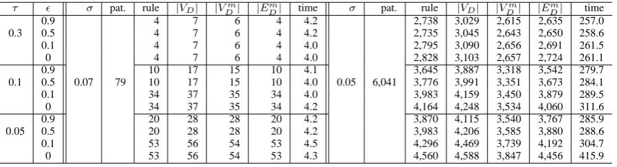
the first experiments. Given several combinations of three thresholds, (i)σ for support value of time patterns, (ii)τ for confidence value of graph evolution rules, and (iii)ϵ for representative time patterns, we measure the number of frequent time patterns and the number of graph evolution rules obtained from representative patterns. In addition, the number of vertices and edges in graph evolution DAGs (DAGGER) as well as abstract graph evolution DAGs (DAGmaxGER) are examined. Note that, the number of edges in a graph evolution DAG is identical with the number of graph evolution rules. In all experiments, fourth threshold δ for representative time patterns was set to 1.
The experimental results are shown in Table II. All results are obtained within a reasonable computation time. Number of discovered frequent time patterns are greatly different between two support threshold σ = 0.07 and σ = 0.05. The same tendency can be observed on the number of graph evolution rules. Compared with σ, thresholds τ and ϵ seem to give small impact on the results. While it does not necessarily to hold because of the greedy algorithm, the number of representative time patterns increases as a thresholdϵbecomes smaller.
We succeeded in compressing a set of frequent time patterns into a small representative set. The numbers of representative patterns are reduced to 26.4% and 59.8% in σ= 0.07 andσ= 0.05, respectively. In case ofσ = 0.05, the number of vertices in the DAGs is reduced to 84.9% in average and to 82.3% in the maximal by the abstraction. Compared with the reduction of the vertices, the reduction rate of edges is very small.
B. Interesting time patterns and graph evolution rules
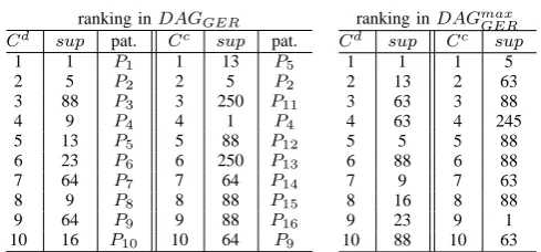
In Table I (left), we show a ranking of top-10 time patterns having high value of centralities in the graph evolution DAG having 419 vertices and 421 edges obtained fromG2 under
the condition ofσ= 0.07,τ= 0.1 andϵ= 0.1.
Since most patterns having high degree centrality consist of two vertices, they correspond to the beginning of graph
TABLE I
RANKING OF TIME PATTERNS W.R.T NETWORK CENTRALITIES
ranking inDAGGER
Cd sup pat. Cc sup pat.
1 1 P1 1 13 P5
2 5 P2 2 5 P2
3 88 P3 3 250 P11
4 9 P4 4 1 P4
5 13 P5 5 88 P12
6 23 P6 6 250 P13
7 64 P7 7 64 P14
8 9 P8 8 88 P15
9 64 P9 9 88 P16
10 16 P10 10 64 P9
ranking inDAGmax GER
Cd sup Cc sup
1 1 1 5
2 13 2 63
3 63 3 88
4 63 4 245
5 5 5 88
6 88 6 88
7 9 7 63
8 16 8 88
9 23 9 1
10 88 10 63
Cd: rank on degree centrality. Cc: rank on closeness centrality.
[image:5.595.307.552.75.189.2]sup: rank on support value. pat.: pattern number in Fig. 7
Fig. 7. Time patterns having high centrality
evolutions. On the other hand, all patterns with high close-ness centrality do not have high support value. And, most patterns ranked in high place consist of more than two ver-tices. Thus, these patterns correspond to certain intermediate steps in graph evolutions. While the concrete time patterns are not shown, a similar tendency can be observed in an abstract graph evolution DAG.
These results show the ability of our proposal to extract time patterns that are difficult to obtain in the traditional support-based framework.
C. Examples of graph evolutions
In Fig. 8, we show examples of the process of graph evolutions found in a time-evolving graphG2under the same
conditions in the second experiments ( σ = 0.07, τ = 0.1 andϵ= 0.1).
In this figure, while the left process (a) is obtained from a graph evolution DAG (DAGGER), the right one (b) represents a process in an abstract graph evolution DAG (DAGmax
TABLE II EXPERIMENTALRESULTS
τ ϵ σ pat. rule |VD| |Vm
D| |EDm| time σ pat. rule |VD| |VDm| |EmD| time
0.9 4 7 6 4 4.2 2,738 3,029 2,615 2,635 257.0
0.3 0.5 4 7 6 4 4.2 2,735 3,045 2,643 2,650 258.6
0.1 4 7 6 4 4.0 2,795 3,090 2,656 2,691 261.5
0 4 7 6 4 4.0 2,828 3,103 2,657 2,724 261.1
0.9 10 17 15 10 4.1 3,645 3,887 3,318 3,542 279.7
0.1 0.5 0.07 79 10 17 15 10 4.0 0.05 6,041 3,776 3,991 3,351 3,673 284.1
0.1 34 37 35 34 4.0 3,983 4,159 3,450 3,879 289.5
0 34 37 35 34 4.2 4,164 4,248 3,534 4,060 311.6
0.9 20 28 28 20 4.2 3,870 4,115 3,540 3,767 285.9
0.05 0.5 20 28 28 20 4.2 3,983 4,206 3,585 3,880 288.6
0.1 53 56 54 53 4.5 4,296 4,469 3,739 4,192 304.7
0 53 56 54 53 4.3 4,560 4,588 3,847 4,456 415.9
pat.: number of discovered time patterns. rule: number of graph evolution rules. |VD|: number of vertices inDAGGER |Vm
D|: number of vertices inDAG max GER. |E
m
D|: number of edges inDAG max
GER. time: execution time in second.
A E To:0 E
Bcc:0
Cc:0
To:4 E To:0 E
Bcc:0
Cc:0
To:2
E To:0 E Bcc:0
Cc:0
To:2
E To:0 E Bcc:0
Cc:0
To:3
A To:4 E To:0 E
Bcc:0
Cc:0
To:3
E To:0 E Bcc:0
Cc:0
E To E
Bcc
Cc
To:2
E To E
Bcc
Cc
To:3
A To:4
E To E
Bcc
Cc
To
(a) (b)
P1a
P2a
P3a
P4a
P5a
P1b
P2b P3b
[image:6.595.76.525.84.206.2]P4b
Fig. 8. Examples of graph evolutions represented in two DAGs
considering the whole structure of a graph pattern as well as the order of edge formation. On the other hand, DAGmax
GER advises us the processes of graph evolutions in an abstract level.
V. RELATEDWORK
Two graph miners GERM[1] and LFR-Miner[6] are the most related work with our proposal. GERM[1] extracts relative time patterns and graph evolution rules in a time-evolving graph. As mentioned previously, our proposal in this paper can be regarded as a modification of [1] by allowing multi-edges in a pattern as well as by changing the definition of confidence. LFR-Miner[6] finds Link formation rules which capture the formation of a new link between specified two vertices as a postcondition of existing con-nections between the two vertices. Link formation rules are closely related to the abstract time patterns. But they are different from the abstract time patterns in the following two points: (i) all edges in a rule must be connected to pre-specified two vertices and (ii) only one edge in a rule is allowed to have the last time period. An abstract time pattern does not have the above restrictions.
VI. CONCLUSIONS ANDFUTUREWORK
In this paper, we propose a framework for discovering interesting patterns and rules in time-evolving graphs. The usefulness of proposed framework was evaluated by prelimi-nary experiments with real world datasets. In the framework,
graph evolution DAGs built from representative and abstract graph evolution rules will help users’ understand by giving an brief overview of discovered patterns and rules. In addition, those DAGs enable us to evaluate the significance of patterns from the aspect of relationships among patterns. In other words, graph evolution DAGs provide additional criteria for pattern discovery other than traditional interestingness measures such as support and confidence.
For future work, further experiments with large-scale datasets and detailed assessment of the quality of obtained graph evolution DAGs are necessary. Furthermore, we in-vestigate to develop a frequent subgraph miner specialized for discovering abstract time patterns having last time-stamp only, i.e. patterns inDAGmax
GER, directly from time-evolving graphs. By combining the rules with detailed time informa-tion and the abstract ones, we can expect to discover useful patterns and rules having appropriate time granularity for capturing important and critical processes in time-evolving graphs.
REFERENCES
[1] M. Berlingerio, F. Bonchi, B. Bringmann and A. Gionis, “Mining Graph Evolution Rules,” in Proc. of the European Conference on Machine Learning and Knowledge Discovery in Databases, Part I, 2009, pp.115–130.
[2] C. Borgelt, “On canonical forms for frequent graph mining”, Working Notes of the Third International ECML/PKDD-Workshop on Mining Graphs, Trees and Sequences, 2005, pp.1–12.
[3] B. Bringmann and S. Nijssen, “What is frequent in a single graph?”, Proc. of the 12th Pacific-Asia Conference on Knowledge Discovery and Data Mining, 2008, pp.858–863.
[4] C. Chen, C. X. Lin and X. Yan and J. Han, “On effective presentation of graph patterns: a structural representative approach”, Proc. of the 17th ACM conference on Information and knowledge management, 2008, pp.299–308.
[5] B. Klimt and Y. Yang, “The enron corpus: A new dataset for email classification research,” in Proc. of the 15th European Conference on Machine Learning, 2004, pp. 217–226.
[6] C. W.-k. Leung, E.-P. Lim, D. Lo and J. Weng, “Mining Interesting Link Formation Rules in Social Networks”, in Proc. of the 19th ACM Conference on Information and Knowledge Management, 2010, pp.209-218.
[7] X. Yan and J. Han, “gSpan : Graph-based substructure pattern mining,” in Proc. of the 2nd IEEE International Conference on Data Mining , 2002, pp. 721–724.