Does the Reserve Options Mechanism really decrease exchange rate volatility? The Synthetic Control Method Approach

Munich Personal RePEc Archive

Does the Reserve Options Mechanism

really decrease exchange rate volatility?

The Synthetic Control Method Approach

Aytug, Huseyin

Bahrain Institute of Banking and Finance

1 January 2016

Online at

https://mpra.ub.uni-muenchen.de/71400/

Does the Reserve Options Mechanism really decrease exchange rate

volatility? The Synthetic Control Method Approach

∗

Huseyin Aytug

January 1, 2016

Abstract

After the invention of the Reserve Option Mechanism (ROM) by the Central Bank of Turkey, it has been debated whether it can help decrease the volatility of foreign exchange rate. In this study, I apply a new microeconometric technique, the synthetic control method, in order to construct a counterfactual foreign exchange rate volatility in the absence of the ROM. I find that, USD/TRY rate is less volatile under the ROM. However, the ROM has not worked efficiently after the announcement of FEDs tapering in May 2013. Furthermore, the ROM could have decreased the volatility of foreign exchange rate if FED had not started tapering.

JEL Codes: C31, E58, F31,

Keywords: FX Intervention, Synthetic Control Method, Required Reserves

∗_{The views expressed herein are solely of the author and do not represent those of Bahrain Institute of Banking and Finance,} its staff or any other institutions. For suggestions and comments, I thank Erdem Basci, Ahmet Bicer, Koray Alper, Fatih Altunok and my former colleagues at the Central Bank of Turkey.

1

Introduction

The invention of the Reserve Option Mechanism (ROM) by the Central Bank of the Republic of Turkey

(CBRT) has shed light on the alternative policy instruments, namely macro-prudential tools, which can be

used to mitigate exchange rate volatility. Between its adaption in September 2011 and FED’s tapering in

June 2013, the level of USD-TR exchange rate and its volatility have both followed a steady path due to the

automatic stabilizer feature of the ROM. However, FED’s tapering caused capital outflows in Turkey like in

other emerging countries and resulted in depreciation of the exchange rate. These developments led people

to ask two main questions? Does the ROM really work? Would the ROM have worked as expected in the

absence of the tapering?

The ROM basically allows banks to hold a certain ratio of their Turkish lira reserve requirements in

foreign exchange and/or gold. It is designed in such a way that it will act as an automatic stabilizer during

capital inflows and outflows. While capital inflows will make foreign exchange relatively cheaper and induce

banks to hold more reserves in foreign exchange, capital outflows will make the Turkish lira relatively cheaper

and induce banks to hold less reserves in foreign exchange. As a consequence, appreciation and depreciation

pressure on the Turkish lira will be eliminated without a need of central bank intervention. Thus, the ROM

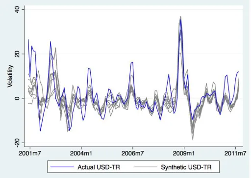
has the potential to decrease exchange rate volatility and act as an automatic stabilizer. Figure 1 shows the

behavior of USD-TRY exchange rate and its volatility.1_{. Both the level and volatility of the exchange rate}

are stabilized until the tapering. However, the Turkish lira kept depreciating and became volatile since the

end of May 2013.

The depreciation of the exchange rate has been mainly caused by the capital outflows but the ROM

should have abolished depreciation pressure as an automatic stabilizer. However, as Aslaner et al. (2015)

argue, CBRT’s systematic response to the tapering by increasing the short term interest rates deteriorated

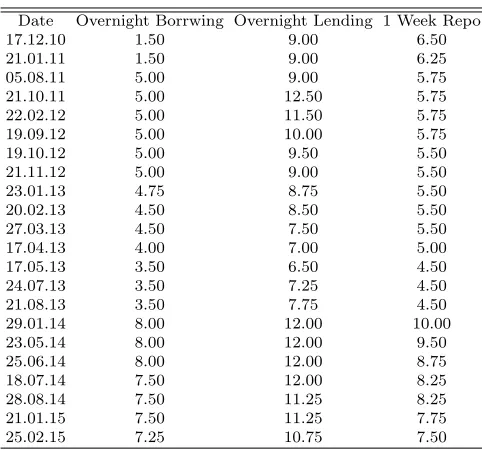
the ROM’s automatic stabilizer feature unexpectedly. CBRT has been using overnight borrowing and lending

interest rates in addition to its policy interest rate, which is 1-Week Repo rate. Table 1 presents the short

term interest rates of CBRT since the establishment of ROM. CBRT initially increased overnight lending

interest rate in July and August 2013 but increased all the short term interest rates drastically in January

2014. Although, CBRT’s main intention was to avert capital outflows, it has also increased the cost of Turkish

lira funding, which has led Turkish banks to hold more reserves in relatively cheaper foreign exchange. Figure

2 illustrates net capital flows and the utilization of the ROM. During the successful phase of the ROM, the

amount of foreign exchange in the ROM increases as Turkey attracts capital flows. After the tapering, the

amount of foreign exchange in the ROM decreases in response capital outflow as expected until August 2013.

However, it started increasing again after CBRT raised the short term interest rates. As a result, the rise

in the utilization of the ROM despite the capital outflows weakened the stabilizer mechanism of the ROM.

In a similar sense, Aslaner et al. (2015) finds that the cost of Turkish lira funding is the underlying driving

force behind the utilization of the ROM. Thus, the behavior of Turkish banks rules out the foreign currency

liquidity concern, which enables the ROM to work as a stabilizer.

The only possible way of estimating the precise impact of the ROM is to construct a counterfactual

exchange rate volatility and calculate the difference between the two. However, this would be only possible if

we had two parallel universes, one with the implemented ROM and one without. We would also need another

universe to investigate whether the ROM could have worked efficiently if FED did not have the tapering. The

synthetic control method (SCM) offers a solution to this problem by constructing a counterfactual exchange

rate volatility with a data-driven method. Thus, the SCM can be used to understand whether the ROM

did really worked until the tapering and could have worked as an automatic stabilizer in the absence of the

tapering

In this study, I construct a counterfactual exchange rate volatility using the SCM and estimate the impact

of the ROM on the exchange rate volatility. I find that the ROM did work efficiently and stabilized the

volatility of the exchange rate until the tapering. I also show that the ROM would have worked better in

the absence of FED’s tapering. My optimization algorithm and placebo tests confirm that my findings are

robust. To the best of my knowledge, this is the first empirical study that utilizes the SCM in assessing the

impact of ROM on exchange rate volatility.

The rest of the paper is organized as follows. While Section 2 details the literature review, Section 3 and

4 present the methodology and the data, respectively. Finally, Section 5 presents the findings and Section 6

concludes the paper.

2

Literature Review

Since the ROM is only used by CBRT, there are only a couple of papers in the literature. Alper et al.

(2013) is a good starting point to understand how the ROM works. They introduce the ROM and compare

it with alternative models. Their findings show that ROM can decrease the exchange rate volatility and it

can be used as a useful policy tool for macroeconomic and financial stability. Kucuksarac and Ozel (2012)

evaluate the ROM and exemplify the calculation of reserve option coefficients. They find that the break-even

coefficients depend on the price of turkish lira and foreign exchange funds and the coefficients are sensitive

to changes in the cost of funds.

to examine the effectiveness of the ROM from an empirical stand of view. Oduncu et al. (2013) is the first

empirical paper in the literature. They basically estimate the effectiveness of the ROM on the exchange

rate volatility using the GARCH model. They find that the ROM is an effective tool to decrease the

volatility. Degerli and Fendoglu (2015) study the impact of the ROM on exchange rate expectations using

the seemingly unrelated regression model. They find that the USD/TL expectations have exhibited lower

levels of volatility after the implementation of the ROM. They also provide evidence that the ROM act as

an automatic stabilizer of expectations. The newest paper is Aslaner et al. (2015), which finds that Turkish

banks are more sensitive to the cost of Turkish funding rather than foreign currency liquidity.They also

argue that CBRT’s adjustment of short term interest rates as a response to capital outflows undermines the

stabilizer feature of the ROM.

3

Methodology

The synthetic control method (SCM) developed by Abadie and Gardeazabal(2003) is a new

microecono-metric technique that has been widely used for comparative case studies. Abadie and Gardeazabal (2003)

implement the SCM to evaluate the effect of terrorism in Spain, Abadie et al. (2010) estimate the effect of

California Tobacco program on tobacco consumption, Lee (2011) studies the inflation targetting and

Nan-nicini and Billimeier (2012) examine the effect of economic liberalization. Using this method, a weighted

combination of control units, the synthetic units, can be used to approximate the characteristics of the

treated unit. In other words, the counterfactual of the treated unit can be constructed in the absence of the

intervention.

Suppose there are J+ 1 units and only the first unit (j= 1) is exposed to intervention after the timeT0

while the otherJ units remain as control units. SetYI

1tas the outcome variable when the unitj= 1 receives

the treatment and YN

1t as the outcome variable in the absence of the treatment at timet ∈ [T0+1, T]. In order to estimateYI

1tandY1Nt Abadie et al. (2010) offer to use the following model:

Yjt=δt+τjtDjt+ ΘtZj+λtφj+ǫjt (1)

whereZjis a vector of independent variables, Θtis a vector of parameters,φj is a pair-specific unobservable,

λtis an unknown common factor,ǫjtis a transitory shock with zero mean andDjtis a dummy variable that

takes value 1 for the treated unit, 0 for the control unit. Then the treatment effect,τ1t, can be estimated

fort=T0+ 1, T0+ 2, ..., T by

τ1t=Y1It−Y N

Even toughYI

1t=Y1tare observable, the estimation of the treatment effect becomes complicated because of

the unobserved control unitYN

1t. Abadie and Gardeazabal (2003) consider a vectorW = (w2, ..., wj+1) such thatwj ≥0 forj= 2, ..., J+ 1 andP

J+1

j=2 wj= 1. In the vector W, each element represents a weight that will

be used to construct a potential synthetic control unit that is approximately same as the treated unit before

the intervention. Hence, for the pre-intervention period (t∈[1, T0]),W∗= (w∗2, ..., wj∗+1) is determined such that

Y1t= J+1

X

j=2

w∗

jYjt (3)

Z1=

J+1

X

j=2

w∗

jZj (4)

where Zjt is a vector of observed covariates not affected by the intervention. Once W∗ is determined, the

treatment effect att=T0+ 1, T0+ 2, ...is estimated as

τ1t=Y1It− J+1

X

j=2

w∗

jYjt (5)

As mentioned above, the weights have to be chosen that the synthetic unit is almost same as the treated unit

before the intervention. LetX1= (Z1, Y11, ..., Y1T0 be a vector of pre-intervention characteristics for the unit j=1 andX0= (Zj, Yjt, ..., YjT0 be a matrix of the same characteristics for the control unitsjǫ[2, J+ 1]. Then the vector W is chosen to minimize the distance betweenX1andX0W subject towj≥0 forj= 2, ..., J+ 1

andw2+...+wJ+1

min

W kX1−X0W kV= minW(V)

q

(X1−X0W)′V(X1−X0W) (6)

In order to solve this minimization problem Abadie et al. (2007) introduce a diagonal and positive

semidef-inite matrix V such that the mean squared prediction error of the outcome variable is minimized over the

control period. The choice of V is very crucial since each diagonal entry reflects the relative importance of

pre-intervention characteristics.

4

Data

Our sample includes 14 emerging countries (Argentina, Brazil, Chile Colombia, Czech Republic, Hungary,

India, Indonesia, Mexico, Poland, Romania, Russia South Africa, and Turkey) and the Euro group. These

countries are selected since they have a similar pattern of current account deficits in the last decade. Our

transfer from the US, and CDS variables for those countries from 2001 M6 to 2014 M9.2 _{All the exchange}

rates are expressed in terms of US dollar. Interest rate differential is defined as the difference between US

and home country interest rate. Inflation differential is also defined in the same manner. Since Argentina,

Romania and Russia are excluded in the estimations since they have either no or larger number of missing

values in interest rate differential.

The measure of exchange rate volatility is critically important since it will influence how well the synthetic

unit approximates the treated unit. While year-over-year changes are too smooth, monthly changes are too

volatile. Thus, I prefer using percentage changes of exchange rates from 3 months before as the volatility

measure.

Exchange rates and inflation are obtained from the IMF. CDSs and interest rates are from Bloomberg.

Finally, asset transfer, which shows financial asset transaction data between the US and a home country,

from the US Treasury TIC data. Asset transfers are normalized with monthly US personal income that is

obtained from the BEA since monthly US GDP data is not available.

5

Results

5.1

The Choice of Control Period

The main purpose of this paper is to estimate the counterfactual trajectory of TR-USD exchange rate

volatility by a convex combination of other currencies. This counterfactual is the hypothetical TR-USD

exchange rate volatility which is assumed to would have existed if the Central Bank of Turkey had not

adopted the ROM after 2011 October. Thus, the period between 2011 October and 2014 November becomes

the treatment period. Choosing the appropriate control period is vital as the optimal weights of other

currencies are estimated in the control period.

One approach in the literature is to use the whole period before the treatment as the control period.

However, it not easy to assume that the whole period before the treatment is the best control period to

approximate the trajectory of TR-USD exchange rate volatility. Cheung et al. (2005) argues that even

well-defined exchange rate models do not work in all sample periods. Thus, I implement a ”rolling optimization”

algorithm in order to find the appropriate control period. That is, regressions are run over a period window

by keeping window size same, then the window is moved up one month forward until the treatment period.

The ”rolling optimization ” is implemented over 1-year, 2-year, 3-year, 4-year and full (the whole period

2_{Although we have observations before 2001 M6, we exclude those because Turkey had a severe financial crises over}

before the treatment) control periods to find the best approximate of the treated exchange rate volatility. As

Inoue (2012) argues the main issue in the optimization process is the explanatory power of the control period.

The explanatory power of control periods is measured by Root Mean Squared Prediction Erros (RMSPE)3

that is provided after the SCM estimations. The smaller RMSPE is a sign of better approximation of the

treated volatility. Additionally, I also check correlation and Adjust R2 between the treated and synthetic

volatility.

It is very important how the optimization works since the estimation of control unit weights and the

synthetic exchange rate volatility purely depends on it. The optimization algorithm minimizes the difference

between observed variables and the synthetic variable that is the weighted average of control units over the

control period. While observed variables, which are shown with subscript j, are the actual observations of

Turkey, the synthetic variable, which is shown with subscript k, are the weighted average of control countries’

observations. CP Ij(k),t is the CPI based inflation differential at time t between the US and the country j

(k),rj(k),t is the interest rate differential at time t between the US and the country j (k),Assetj(k) is the

net asset transaction between the US and the country j (k) divided by US personal income,CDSj(k) is the

CDS of country j (k) at time t. J P Yt is the TR-USD percent change from 3 months before at time t and

Sj,t is the weighted of control currencies’ percent change from 3 months before at time t. The upper bar

on variables represents a simple average over the control period. The optimization algorithm used for the

estimation of optimal weights is as follows;

min

w2,...,wj+1

CP Ij−Pk=2wkCP Ik

rj−Pk=2wkrk

Assetj−Pk=2wkAssetk

CDSj−Pk=2wkCDSk

J P Y0−Pk=2wkSk,0

J P Y1−Pk=2wkSk,1 ..

.

J P YT0−

P

k=2wkSk,12

(7)

Among 380 control groups, I chose 2 periods from 1-year, 2-year, 3-year and 4-year control periods that

have the lowest RMSPE, highest Adj2R and highest correlation. I also include full control period. Table

2 presents 9 optimal control periods and reveals that correlations and AdjR2s are similar while RMSPE

decreases when the window size expands. Thus, I choose the period over 2007M3-2008M2 as the control

3_{RMSPE is estimated as}

s T P

t

(YI 1t−Y1Nt)

2

period since it has the minimum RMSPE, high correlation and Adj2

R. The weights that are obtained for

the control period is presented in Table 3. Based on the minimization process, the volatility of TR-USD

exchange rate can be duplicated by the convex combination of the Brazilian Real, the Czech Krone and the

South African dollar. The estimated weights are 0.74, 0.126, and 0.134, respectively.

The weights of the control currencies are estimated using predictor variables of the TR-USD exchange

rate, which are interest rate spreads, asset transfers, CPI inflation differential, and the volatility of the

TR-USD exchange rate at different periods. Both predictor variables and the outcome variable are well

balanced during the optimization process between the synthetic control and treatment units. In other

words, the difference between actual and synthetic values of these variables are very close to each other. The

predictor balance over the optimization process and the importance of each variable are presented in Table 4.

Importance of a variables represents the relative importance of each predictor variable, which are normalized

weights in constructing the synthetic control units. Volatility of TR-USD exchange rate in different periods

seem to be relatively important compared to the macro variables. While the normalized weight of macro

variables are smaller than 1 percent, the volatility of TR-USD exchange rate in each month has a normalized

weight of 10 percent on average.

5.2

Average Treatment Effects

In Figure 4 and 5, I calculate the average treatment effect of the reserve option mechanism by taking the

difference between the actual and synthetic volatility TR-USD exchange rate. The positive(negative) sign of

ATE stands represents that the ROM works efficiently (not efficiently). The effect of the ROM is evaluated

as efficient when TR-USD exchange rate has a lower volatility. Thus, smaller depreciation and appreciation

under the ROM will be both considered as efficient. However, there are some periods that while the actual

TR-USD exchange rate depreciates, the synthetic one appreciates. For these periods, the absolute value

of the volatility is taken and then the difference is estimated in order to be consistent with the evaluation

criterion.

It is shown that ATEs are mainly positive until the FED’s tapering in May 2013 and mainly negative

after that. The average of ATEs until May 2013 is 2.5 percent and it becomes -1.15 afterwards, which is an

evidence that the ROM works. These results confirm that the ROM had worked efficiently as an automatic

stabilizer and decreased the volatility until the FED’s Tapering. The findings here are consistent with those

in Oduncu et al (2013) and Degerli and Fendoglu (2013). I re-calculate the synthetic TR-USD exchange rate

by including the credit swap defaults (CDS) as a predictor variable the findings are very similar. Likewise the

While the average of ATEs until May 2013 is 2.28 percent, it becomes -1.34 afterwards. The alternative

estimation with CDSs confirm my initial findings that the ROM had worked efficiently until May 2013.

The puzzle that why the ROM stopped working efficiently after May 2013 is worth investigating. Aslaner

et al. (2015) investigate the the determinants of ROM utilization and find that foreign currency liquidity is

not an important parameter for ROM utilization, which is in contrast to the mechanism of ROM. As argued

in Alper et al (2013), the ROM is expected to work as an automatic stabilizer if banks act accordingly with

foreign currency liquidity constraint. They also argue that the policy induced movements in the short term

interest rates may mitigate the efficiency of the ROM. Thus, the puzzle can be investigated by examining

how the CBRT changed its short term interest rates after the FED’s tapering. The CBRT has mainted a

stable monetary policy between the implementation of ROM and the FED’s tapering. It kept the policy

interest rate, which 1 week repo interest rate and the interest corridor, which is overnight borrowing and

lending interest rates around the same level. Thus, there was a small variation in interest rates during the

efficient phase of the ROM. However, after August 2013, the CBRT started increasing short term interest

rates to stop capital outflows, which is induced by the FED’s tapering. The increase in the short term

interest rates raised the cost of Turkish lira funding that is believed to be the important driving force of high

ROM utilization of Turkish banks after the FED’s tapering. As a result, the increase in short term interest

rates during capital outflows deteriorated the automatic stabilizer function of the ROM.

5.3

A World without the FED’s tapering

The puzzle caused by the CBRT’s respond to capital outflows can be investigated by estimating the

synthetic TR-USD exchange rate if the CBRT had not increased the short term interest rates. Since the

ROM had worked efficiently between October 2011 and August 2013, this period can be used a control period

and the synthetic TR-USD exchange rate can be re-estimated for the period after July 2013. Likewise, the

length of optimization period is vital since the weights estimated in the optimization period will be used

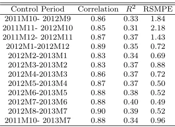
for the construction of synthetic TR-USD exchange rate. I re-optimze the control periods for different

1-year periods and full control period. The estimated RSMPE’s andAdj2

Rs are given in Table 5. Among 12

optimizations, the control period between 2012 M6 and 2013 M5 has the smallest RSMPE and relatively

highAdj2_R. The weights that are estimated using this control period are given in Table 6. Thus, the synthetic volatility of TR-USD exchange rate can be calculated by the convex combination of Chilean Peso, Colombian

Peso, the Euro, Hungarian Forint and Mexican Peso. The estimated weights are 0.136, 0.643, 0.049, 0.78 and

0.94, respectively. Predictor balance of the new optimization is given in Table 7. Like the ROM optimization,

rather than macro variables.

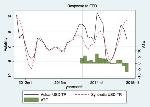
The volatility of actual and synthetic TR-USD exchange are plotted in Figure 7. I also calculate the

average treatment effect for the treatment period by taking the difference between the actual and synthetic

volatility TR-USD exchange rate, which is shown in Figure 7. ATEs are positive until the last two months,

which confirms that the ROM would have worked efficiently if the CBRT had not increased short term interest

rates systematically. The average of ATEs for the treatment period is 2 percent. When the estimation is

iterated by including the credit swap defaults (CDS) as a predictor variable, I estimate similar results. Thus,

the findings are robust.

5.4

Placebo Study

Using the SCM, I estimate the counterfactual USD-TR exchange rate volatility, which is percent changes

from 3 months before, by a convex combinations of currencies of 10 different countries. There is a possibility

that my estimation could be driven by chance. Thus, I run placebo tests to check the robustness of my

estimates. The placebo test helps answering whether I would estimate similar effects if I had chosen a

random country from the dataset.

Following Abadie and Gardeazabal (2003) and Abadie et al. (2010), I estimate the synthetic exchange

rate volatility for countries in the control group. If the placebo studies generate similar results for other

currencies, then the volatility of USD-TR exchange rate was stabilized by other factors than the automatic

stabilizer feature of the ROM. Otherwise, my results provide significance and robust evidence for the ROM’s

ability to decrease the exchange rate volatility.

Table 8 shows pre RMSPE, post RMSP, the ratio of post and pre RSMPEs and average ATE for Turkish

lira and other currencies. The average gap between the synthetic and actual volatility of the exchange rate is

expected to be close or less than 0 for other currencies. Especially, Brazillian Real, Czech Krone and South

African Rand are of importance since their weights are different than 0 in the construction of synthetic

volatility of USD-TR exchange rate. While the average gap is negative for Brazillian Real and South African

Rand, it is very close to zero for Czech Krone. Based on the placebo tests, we can confirm that my estimation

are robust in estimating the impact of the ROM on the exchange rate volatility.

The placebo test results for the tapering are shown in Table 9. The average between rhe synthetic and

actual volatility of the USD-TR exchange rate is 2 percent and the average gap for control currencies that are

Chilean Peso, Columbian Peso, the Euro, Hungarian Forint and Mexican Peso should be smaller. As shown

in Table 9, the average gap for control currencies is smaller than 2 percent and is close to zero for the most

than control currencies. These results reveal that I chose the right control currencies in my optimization

process. Thus, my estimation are significant and robust, which confirms that the ROM could have worked

efficiently in the absence of the tapering.

6

Conclusion

The ROM is an important macroprudential tool, which has been used by the CBRT to stabilize the

exchange rate volatility.It had worked efficiently and decreased the volatility of the USD-TR exchange rate

until the FED’s tapering in May 2013 . However, CBRT’s change in short term interest rates as a response

to stop capital flows deteriorated the automatic stabilizer feature of the ROM. Thus, the volatility of the

exchange rate was not stabilized after the tapering. In this paper, I use the Synthetic Control Method

to confirm that the ROM had worked as an automatic stabilizer until the tapering. To the best of my

knowledge, this is the first application of that methodology to investigate the ROM.

My results indicate that the ROM decreased the exchange rate volatility by 2 percentage points on

average and the estimated cumulative effect is around 50 percentage points between September 2011 and

August 2013. However, the ROM did not work efficiently after August 2013 caused by the behavior of

Turkish banks in response to changes in short term interest rates. My estimates also reveals that the ROM

could have worked as expected and stabilized the exchange rate volatility in the absence of the tapering.

The ROM could have decreased the exchange rate volatility by 2 percentage points on average and volatility

could have been decreased by 32 percentage points cumulatively after the tapering. Robustness of both

results are confirmed via placebo study as well.

Our results are consistent with the general view in the literature that the ROM can decrease exchange

rate volatility. However, the ROM can work efficiently when CBRT does not change short term interest rate

during capital outflows. The reason is that the behavior of the Turkish banks is strongly determined by the

Figure 1: USD-TRY Exchange Rate

Figure 2: Capital Flows and FX Reserves in ROM. Source: CBRT

Figure 4: Actual and Synthethic USD-TR Exchange Rate

Figure 5: Actual and Synthethic USD-TR Exchange Rate and Average Treatment Effects

Figure 7: Actual and Synthethic USD-TR Exchange Rate and Average Treatment Effects

Table 1: CBRT Interest Rates

Date Overnight Borrwing Overnight Lending 1 Week Repo

17.12.10 1.50 9.00 6.50

21.01.11 1.50 9.00 6.25

05.08.11 5.00 9.00 5.75

21.10.11 5.00 12.50 5.75

22.02.12 5.00 11.50 5.75

19.09.12 5.00 10.00 5.75

19.10.12 5.00 9.50 5.50

21.11.12 5.00 9.00 5.50

23.01.13 4.75 8.75 5.50

20.02.13 4.50 8.50 5.50

27.03.13 4.50 7.50 5.50

17.04.13 4.00 7.00 5.00

17.05.13 3.50 6.50 4.50

24.07.13 3.50 7.25 4.50

21.08.13 3.50 7.75 4.50

29.01.14 8.00 12.00 10.00

23.05.14 8.00 12.00 9.50

25.06.14 8.00 12.00 8.75

18.07.14 7.50 12.00 8.25

28.08.14 7.50 11.25 8.25

21.01.15 7.50 11.25 7.75

25.02.15 7.25 10.75 7.50

Table 2: Control Periods for ROM

Control Period Correlation R2 RSMPE 2007M3-2008M2 0.74 0.54 1.06 2010M1-2010M12 0.65 0.42 1.06 2005M8-2007M4 0.64 0.40 2.79 2008M12-2010M11 0.57 0.32 2.57 2003M9-2006M8 0.76 0.57 6.06 2005M11-2008M10 0.75 0.56 6.17 2003M4-2007M3 0.75 0.56 6.22 2006M9-2010M8 0.73 0.54 6.29 2001M6-2011M9 0.74 0.54 6.41

Table 3: Currency Weights for ROM

Table 4: Predictor Balance for ROM

Variable Treated Synthetic Importance

CP I_jt _{-5.37875 -1.238373 0.0014311} r_jt _{-12.1515 -5.625667 0.0090698}

Asset_jt 0.1489167 0.8200997 0.0002259

T RL₁ -1.611773 -1.412259 0.0434617

T RL_{2 -4.708365 -4.227849 0.0367692} T RL_{3 -4.235464 -4.788174 0.0581586} T RL_{4 -6.125362 -5.846677 0.1186323} T RL₅ -5.604718 -5.7288 0.1100892

T RL₆ -1.424283 -0.4320435 0.1139845

T RL_{7 -4.476481 -2.150733 0} T RL_{8 -6.718748 -4.50028 0} T RL_{9 -9.733842 -9.755344 0.1953708} T RL₁0 -6.910238 -6.187835 0.1180902

T RL₁1 -1.842542 -1.563376 0

T RL_{12 0.4212296 -0.5087929 0.1947169}

Table 5: Control Periods for Tapering

Control Period Correlation R2 RSMPE 2011M10- 2012M9 0.86 0.33 1.84 2011M11- 2012M10 0.85 0.31 2.18 2011M12- 2012M11 0.87 0.37 1.43 2012M1-2012M12 0.89 0.35 0.72 2012M2-2013M1 0.83 0.34 0.69 2012M3-2013M2 0.83 0.37 0.88 2012M4-2013M3 0.86 0.37 0.72 2012M5-2013M4 0.87 0.37 0.50 2012M6-2013M5 0.88 0.38 0.52 2012M7-2013M6 0.88 0.40 0.49 2012M8-2013M7 0.90 0.39 0.52 2011M10- 2013M7 0.88 0.34 0.96

Table 6: Currency Weights for Tapering

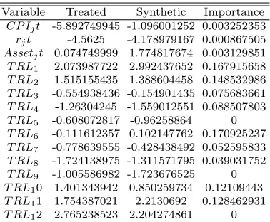
Table 7: Predictor Balance for Tapering

Variable Treated Synthetic Importance

CP I_jt -5.892749945 -1.096001252 0.003252353

r_jt -4.5625 -4.178979167 0.000867505

Asset_jt 0.074749999 1.774817674 0.003129851

T RL_{1 2.073987722 2.992437652 0.167915658} T RL_{2 1.515155435 1.388604458 0.148532986} T RL₃ -0.554938436 -0.154901435 0.075683661

T RL₄ -1.26304245 -1.559012551 0.088507803

T RL₅ -0.608072817 -0.96258864 0

T RL_{6 -0.111612357 0.102147762 0.170925237} T RL_{7 -0.778639555 -0.428438492 0.052595833} T RL_{8 -1.724138975 -1.311571795 0.039031752} T RL₉ -1.005586982 -1.723676525 0

T RL₁0 1.401343942 0.850259734 0.12109443

T RL_{11 1.754387021 2.2130692 0.128462931} T RL_{12 2.765238523 2.204274861 0}

Table 8: Placebo Test Results for ROM

Turkey Brazil Chile Columbia Czech Rep Euro Hungary India Indonesia Mexico Poland South Africa pre RSMPE 6.55 7.48 5.21 4.44 3.49 3.06 3.84 4.21 5.91 4.86 3.93 7.96 post RSMPE 4.58 5.96 2.16 5.06 2.18 3.56 4.13 4.54 4.74 3.18 2.27 5.11 post/pre 0.70 0.80 0.41 1.14 0.62 1.17 1.08 1.08 0.80 0.65 0.58 0.64 Average ATE 2.50 -2.04 -0.09 1.78 0.18 1.16 -1.30 -1.78 2.36 -1.67 -1.05 -1.26

Table 9: Placebo Test Results for Tapering

References

Alberto Abadie, Alexis Diamond, and Jens Hainmueller. Synthetic control methods for comparative case

studies: Estimating the effect of californias tobacco control program. Journal of the American Statistical

Association, 105(490), 2010.

Alberto Abadie and Javier Gardeazabal. The economic costs of conflict: A case study of the basque country.

American economic review, pages 113–132, 2003.

Koray Alper, Hakan Kara, and Mehmet Y¨or¨uko˘glu. Reserve options mechanism. Central Bank Review,

13(1), 2012.

Oguz Aslaner, Ugur Ciplak, Hakan Kara, and Doruk Kucuksarac. Reserve option mechanism: Does it work

as an automatic stabilizer? Central Bank Review, 15(1), 2015.

Andreas Billmeier and Tommaso Nannicini. Assessing economic liberalization episodes: A synthetic control

approach. Review of Economics and Statistics, 95(3):983–1001, 2013.

N Campos, Fabrizio Coricelli, and Luigi Moretti. Economic growth and political integration: Synthetic

counterfactuals evidence from europe. Technical report, mimeo, 2014.

Marcos Chamon, M´arcio Garcia, and Laura Souza. Fx interventions in brazil: a synthetic control approach.

Technical report, 2015.

Ahmet De˘gerli and Salih Fendo˘glu. Reserve option mechanism as a stabilizing policy tool: Evidence from

exchange rate expectations. International Review of Economics & Finance, 35:166–179, 2015.

Pedro Gomis-Porqueras and Laura Puzzello. Winners and losers from the euro.

Doruk K¨u¸c¨uksara¸c and ¨Ozg¨ur ¨Ozel. Reserve options mechanism and computation of reserve options

coeffi-cients. TCMB Ekonomi Notu, (12/33), 2012.

Wang-Sheng Lee. Comparative case studies of the effects of inflation targeting in emerging economies.Oxford

Economic Papers, page gpq025, 2010.

Arif Oduncu, Yasin Akcelik, and Ergun Ermisoglu. Reserve options mechanism and fx volatility. Central