Exploring the Relative Role of Bottom-up and Top-down Information in
Phoneme Learning
Abdellah Fourtassi1, Thomas Schatz1,2, Balakrishnan Varadarajan3, Emmanuel Dupoux1 1 Laboratoire de Sciences Cognitives et Psycholinguistique, ENS/EHESS/CNRS, Paris, France
2SIERRA Project-Team, INRIA/ENS/CNRS, Paris, France 3Center for Language and Speech Processing, JHU, Baltimore, USA
{abdellah.fourtassi; emmanuel.dupoux; balaji.iitm1}@gmail
Abstract
We test both bottom-up and top-down ap-proaches in learning the phonemic status of the sounds of English and Japanese. We used large corpora of spontaneous speech to provide the learner with an input that models both the linguistic properties and statistical regularities of each language. We found both approaches to help dis-criminate between allophonic and phone-mic contrasts with a high degree of accu-racy, although top-down cues proved to be effective only on an interesting subset of the data.
1 Introduction
Developmental studies have shown that, during their first year, infants tune in on the phonemic cat-egories (consonants and vowels) of their language, i.e., they lose the ability to distinguish some within-category contrasts (Werker and Tees, 1984) and enhance their ability to distinguish between-category contrasts (Kuhl et al., 2006). Current work in early language acquisition has proposed two competing hypotheses that purport to account for the acquisition of phonemes. The bottom-up hypothesisholds that infants converge on the lin-guistic units of their language through a similarity-based distributional analysis of their input (Maye et al., 2002; Vallabha et al., 2007). In contrast, the top-down hypothesis emphasizes the role of higher level linguistic structures in order to learn the lower level units (Feldman et al., 2013; Mar-tin et al., 2013). The aim of the present work is to explore how much information can ideally be derived from both hypotheses.
The paper is organized as follows. First we de-scribe how we modeled phonetic variation from audio recordings, second we introduce a bottom-up cue based on acoustic similarity and top-down cues based of the properties of the lexicon.
We test their performance in a task that consists in discriminating within-category contrasts from between-category contrasts. Finally we discuss the role and scope of each cue for the acquisition of phonemes.
2 Modeling phonetic variation
In this section, we describe how we modeled the representation of speech sounds putatively pro-cessed by infants, before they learn the relevant phonemic categories of their language. Following Peperkamp et al. (2006), we make the assumption that this input is quantized into context-dependent phone-sized unit we callallophones. Consider the example of the allophonic rule that applies to the French /r/:
/r/→
[X]/ before a voiceless obstruent [K] elsewhere
Figure 1: Allophonic variation of French /r/
The phoneme /r/ surfaces as voiced ([K]) before a voiced obstruent like in [kanaK Zon] (“canard jaune”, yellow duck) and as voiceless ([X]) before a voiceless obstruent as in [kanaX puXpK] (“ca-nard pourpre”, purple duck). Assuming speech sounds are coded as allophones, the challenge fac-ing the learner is to distfac-inguish the allophonic vari-ation ([K], [X]) from the phonemic variation (re-lated to a difference in the meaning) like the con-trast ([K],[l]).
Previous work has generated allophonic varia-tion using random contexts (Martin et al., 2013). This procedure does not take into account the fact that contexts belong to natural classes. In addition, it does not enable to compute an acoustic distance. Here, we generate linguistically and acoustically controlled allophones using Hidden Markov Mod-els (HMMs) trained on audio recordings.
2.1 Corpora
We use two speech corpora: the Buckeye Speech corpus (Pitt et al., 2007), which consists of 40 hours of spontaneous conversations with 40 speak-ers of American English, and the core of the Cor-pus of Spontaneous Japanese (Maekawa et al., 2000) which also consists of about 40 hours of recorded spontaneous conversations and public speeches in different fields. Both corpora are time-aligned with phonetic labels. Following Boruta (2012), we relabeled the japanese corpus using 25 phonemes. For English, we used the phonemic version which consists of 45 phonemes.
2.2 Input generation
2.2.1 HMM-based allophones
In order to generate linguistically and acoustically plausible allophones, we apply a standard Hidden Markov Model (HMM) phoneme recognizer with a three-state per phone architecture to the signal, as follows.
First, we convert the raw speech waveform of the corpora into successive vectors of Mel Fre-quency Cepstrum Coefficients (MFCC), computed over 25 ms windows, using a period of 10 ms (the windows overlap). We use 12 MFCC coeffi-cients, plus the energy, plus the first and second or-der or-derivatives, yielding 39 dimensions per frame. Second, we start HMM training using one three-state model per phoneme. Third, each phoneme model is cloned into context-dependent triphone models, for each context in which the phoneme actually occurs (for example, the phoneme /A/ oc-curs in the context [d–A–g] as in the word /dAg/ (“dog”). The triphone models are then retrained on only the relevant subset of the data, corresponding to the given triphone context. These detailed mod-els are clustered back into inventories of various sizes (from 2 to 20 times the size of the phone-mic inventory) using a linguistic feature-based de-cision tree, and the HMM states of linguistically similar triphones are tied together so as to max-imize the likelihood of the data. Finally, the tri-phone models are trained again while the initial gaussian emission models are replaced by mix-ture of gaussians with a progressively increasing number of components, until each HMM state is modeled by a mixture of 17 diagonal-covariance gaussians. The HMM were built using the HMM Toolkit (HTK: Young et al., 2006).
2.2.2 Random allophones
As a control, we also reproduce the random al-lophones of Martin et al. (2013), in which allo-phonic contexts are determined randomly: for a given phoneme /p/, the set of all possible con-texts is randomly partitioned into a fixed number
nof subsets. In the transcription, the phoneme/p/
is converted into one of its allophones (p1,p2,..,pn) depending on the subset to which the current con-text belongs.
3 Bottom-up and top-down hypotheses 3.1 Acoustic cue
The bottom-up cue is based on the hypothesis that instances of the same phoneme are likely to be acoustically more similar than instances of two different phonemes (see Cristia and Seidl, in press) for a similar proposition). In order to provide a proxy for the perceptual distance between al-lophones, we measure the information theoretic distance between the acoustic HMMs of these al-lophones. The 3-state HMMs of the two allo-phones were aligned with Dynamic Time Warping (DTW), using as a distance between pairs of emit-ting states, a symmetrized version of the Kullback-Leibler (KL) divergence measure (each state was approximated by a single non-diagonal Gaussian):
A(x, y) =
X
(i,j)∈DTW(x,y)
KL(Nxi||Nyj) +KL(Nyj||Nxi)
Where{(i, j) ∈ DTW(x, y)} is the set of in-dex pairs over the HMM states that correspond to the optimal DTW path in the comparison between phone modelxandy, andNxi the full covariance
Gaussian distribution for stateiof phone x. For obvious reasons, the acoustic distance cue cannot be computed for Random allophones.
3.2 Lexical cues
next sound is a voiceless obstruent. Therefore, the lexical item /kanar/ surfaces as [kanaX] or [kanaK]. The lexical cue assumes that a pair of words dif-fering in the first or last segment (like [kanaX] and [kanaK]) is more likely to be the result of a phono-logical process triggered by adjacent sounds, than a true semantic minimal pair.
However, this strategy clearly gives rise to false alarms in the (albeit relatively rare) case of true minimal pairs like [kanaX] (“duck”) and [kanal] (“canal”), where ([X], [l]) will be mistakenly la-beled as allophonic.
In order to mitigate the problem of false alarms, we also use Boruta (2011)’s continuous version, where each pair of phones is characterized by the number of lexical minimal pairs it forms.
B(x, y) =|(Ax, Ay)∈L2|+|(xA, yA)∈L2|
where{Ax∈L}is the set of words in the lex-iconLthat end in the phonex, and{(Ax, Ay) ∈
L2} is the set of phonological minimal pairs in L×Lthat vary on the final segment.
In addition, we introduce another cue that could be seen as a normalization of Boruta’s cue:
N(x, y) = |{Ax∈L|(Ax,Ay)}|+|{Ay∈∈LL}|2|++||{(xA,yA)xA∈L}|∈+L|{2|yA∈L}|
4 Experiment 4.1 Task
For each corpus we list all the possible pairs of attested allophones. Some of these pairs are allo-phones of the same phoneme (allophonic pair) and others are allophones of different phonemes (non-allophonic pairs). The task is a same-different classification, whereby each of these pairs is given a score from the cue that is being tested. A good cue gives higher scores to allophonic pairs. 4.2 Evaluation
We use the same evaluation procedure as in Mar-tin et al. (2013). It is carried out by compuMar-ting the area under the curve of the Receiver Operat-ing Characteristic (ROC). A value of 0.5 repre-sents chance and a value of 1 reprerepre-sents perfect performance.
In order to lessen the potential influence of the structure of the corpus (mainly the order of the ut-terances) on the results, we use a statistical resam-pling scheme. The corpus is divided into small blocks (of 20 utterances each). In each run, we draw randomly with replacement from this set of
blocks a sample of the same size as the original corpus. This sample is then used to retrain the acoustic models and generate a phonetic inven-tory that we use to re-transcribe the corpus and re-compute the cues. We report scores averaged over 5 such runs.
[image:3.595.321.504.285.344.2]4.3 Results
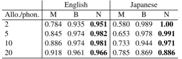
Table 1 shows the classification scores for the lex-ical cues when we vary the inventory size from 2 allophones per phoneme in average, to 20 al-lophones per phoneme, using the Random allo-phones. The top-down scores are very high, repli-cating Martin et al.’s results, and even improving the performance using Boruta’s cue and our new Normalized cue.
— English Japanese Allo./phon. M B N M B N 2 0.784 0.935 0.951 0.580 0.989 1.00 5 0.845 0.974 0.982 0.653 0.978 0.991 10 0.886 0.974 0.981 0.733 0.944 0.971 20 0.918 0.961 0.966 0.785 0.869 0.886 Table 1 : Same-different scores for top-down cues on Random allophones, as a function of the average number of
allophones per phoneme. M=Martin et al., B=Boruta, N= Normalized
Table 2 shows the results for HMM-based allo-phones. The acoustic score is very accurate for both languages and is quite robust to variation. Top-down cues, on the other hand, perform, sur-prisingly, almost at chance level in distinguish-ing between allophonic and non-allophonic pairs. A similar discrepancy for the case of Japanese was actually noted, but not explained, in Boruta (2012).
— English Japanese
[image:3.595.310.526.547.607.2]Allo./phon. A M B N A M B N 2 0.916 0.592 0.632 0.643 0.885 0.422 0.524 0.537 5 0.918 0.592 0.607 0.611 0.908 0.507 0.542 0.551 10 0.893 0.569 0.571 0.571 0.827 0.533 0.546 0.548 20 0.879 0.560 0.560 0.559 0.876 0.541 0.543 0.543
Table 2 : Same-different scores for bottom-up and top-down cues on HMM-based allophones, as a function of the average number of allophones per phoneme. A=Acoustic,
M=Martin et al., B=Boruta, N= Normalized
5 Analysis
5.1 Why does the performance drop for realistic allophones?
lexi-cal alternants ([X], [K]) →([kanaX] and [kanaK]), others to true minimal pairs ([K], [l])→([kanaK] and [kanal]), and yet others will simply not gen-erate lexical variation at all, we will call those:
invisible pairs. For instance, in English, /h/ and /N/ occur in different syllable positions and thus cannot appear in any minimal pair. As defined above, top-down cues are set to 0 in such pairs (which means that they are systematically classi-fied as non-allophonic). This is a correct decision for /h/ vs. /N/, but not for invisible pairs that also happen to be allophonic, resulting in false nega-tives. In tables 3, we show that, indeed, invisible pairs is a major issue, and could explain to a large extent the pattern of results found above. In fact, the proportion of visible allophonic pairs (“allo” column) is way lower for HMM-based allophones. This means that the majority of allophonic pairs in the HMM case are invisible, and therefore, will be mistakenly classified as non-allophonic.
— Random HMM
[image:4.595.81.280.343.412.2]— English Japanese English Japanese Allo./phon. allo ¬allo allo ¬allo allo ¬allo allo ¬allo 2 92.9 36.3 100 83.9 48.9 25.3 37.1 53.2 5 97.2 28.4 99.6 69.0 31.1 14.3 25.0 25.9 10 96.8 19.9 96.7 50.1 19.8 4.23 21.0 14.4 20 94.3 10.8 83.4 26.4 14.0 1.89 12.4 4.04
Table 3 : Proportion (in %) of allophonic pairs (allo), and non-allophonic pairs (¬allo) associated with at least one lexical minimal pair, in Random and HMM allophones.
There are basically two reasons why an allo-phonic pair would be invisible ( will not generate lexical alternants). The first one is the absence of evidence, e.g., if the edges of the word with the underlying phoneme do not appear in enough con-texts to generate the corresponding variants. This happens when the corpus is so small that no word ending with, say, /r/ appears in both voiced and voiceless contexts. The second, is when the allo-phones are triggered on maximally different con-texts (on the right and the left) as illustrated below:
/p/→
[p1]/A B
[p2]/C D
When A doesn’t overlap with C and B does not overlap with D, it becomes impossible for the pair ([p1], [p2]) to generate a lexical minimal pair. This
is simply because a pair of allophones needs to share at least one context to be able to form vari-ants of a word (the second or penultimate segment of this word).
When asked to split the set of contexts in two distinct categories that trigger [p1] and [p2] (i.e., A BandC D), the random procedure will of-ten make A overlap with B and C overlap with D because it is completely oblivious to any acous-tic or linguisacous-tic similarity, thus making it always possible for the pair of allophones to generate lex-ical alternants. A more realistic categorization (like the HMM-based one), will naturally tend to minimize within-category distance, and maximize between-category distance. Therefore, we will have less overlap, making the chances of the pair to generate a lexical pair smaller. The more al-lophones we have, the bigger is the chance to end up with non-overlapping categories (invisible allo-phonic pairs), and the more mistakes will be made, as shown in Table 3.
5.2 Restricting the role of top-down cues The analysis above shows that top-down cues can-not be used to classify all contrasts. The approxi-mation that consists in considering all pairs that do not generate lexical pairs as non-allophonic, does not scale up to realistic input. A more intuitive, but less ambitious, assumption is to restrict the scope of top-down cues to contrasts that do gen-erate lexical variation (lexical alternants or true minimal pairs). Thus, they remain completely ag-nostic to the status of invisible pairs. This restric-tion makes sense since top-down informarestric-tion boils down to knowing whether two word forms belong to the same lexical category (reducing variation to allophony), or to two different categories (varia-tion is then considered non-allophonic). Phonetic variation that does not cause lexical variation is, in this particular sense, orthogonal to our knowledge about the lexicon.
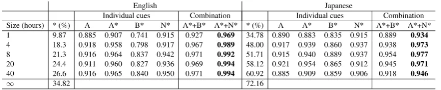
We test this hypothesis by applying the cues only to the subset of pairs that are associated with at least one lexical minimal pair. We vary the num-ber of allophones per phoneme on the one hand (Table 4) and the size of the input on the other hand (Table 5). We refer to this subset by an aster-isk (*), by which we also mark the cues that apply to it. Notice that, in this new framing, the M cue is completely uninformative since it assigns the same value to all pairs.
— English Japanese
[image:5.595.83.509.63.132.2]— — Individual cues Combination — Individual cues Combination Allo./phon. * (%) A A* B* N* A*+B* A*+N* * (%) A A* B* N* A*+B* A*+N* 2 26.6 0.916 0.965 0.840 0.950 0.971 0.994 60.92 0.885 0.909 0.859 0.906 0.918 0.946 4 14.3 0.918 0.964 0.858 0.951 0.975 0.991 30.88 0.908 0.917 0.850 0.936 0.934 0.976 10 4.24 0.893 0.937 0.813 0.939 0.960 0.968 16.06 0.827 0.839 0.899 0.957 0.904 0.936 20 1.67 0.879 0.907 0.802 0.907 0.942 0.940 5.02 0.876 0.856 0.882 0.959 0.913 0.950
Table 4 : Same-different scores for different cues and their combinations with HMM-allophones, as a function of average number of allophones per phonemes.
— English Japanese
— — Individual cues Combination — Individual cues Combination Size (hours) * (%) A A* B* N* A*+B* A*+N* * (%) A A* B* N* A*+B* A*+N* 1 9.87 0.885 0.907 0.741 0.915 0.927 0.969 34.78 0.890 0.883 0.835 0.915 0.889 0.934 4 18.3 0.918 0.958 0.798 0.917 0.967 0.989 48.00 0.917 0.939 0.860 0.937 0.938 0.973 8 21.3 0.916 0.964 0.837 0.942 0.971 0.992 51.71 0.915 0.940 0.889 0.937 0.954 0.977 20 24.4 0.911 0.960 0.827 0.936 0.969 0.994 58.12 0.921 0.954 0.865 0.912 0.945 0.971 40 26.6 0.916 0.965 0.840 0.950 0.971 0.994 60.92 0.885 0.909 0.859 0.906 0.918 0.946
∞ 34.82 — — — — — — 72.16 — — — — — —
Table 5 : Same-different scores for different cues and their combinations with HMM-allophones, as a function of corpus size. * (%) refers to the proportion of the subset of contrasts associated with at least one minimal pair. The cues applied to this
subset are marked with an asterisk (*)
information are not completely redundant. How-ever, the scope of top-down cues (the proportion of the subset * ) shrinks as we increase the number of allophones. Table 5 shows that this problem can, in principle, be mitigated by increasing the amount of data available to the learner. As we were limited to only 40 hours of speech, we generated an artifi-cial corpus that uses the same lexicon but with all possible word orders so as to maximize the num-ber of contexts in which words appear. This artifi-cial corpus increases the proportion of the subset, but we are still not at 100 % coverage, which ac-cording the analysis above, is due (at least in part) to the irreducible set of non-overlapping pairs.
6 Conclusion
In this study we explored the role of both bottom-up and top-down hypotheses in learning the phonemic status of the sounds of two typologically different languages. We introduced a bottom-up cue based on acoustic similarity, and we used al-ready existing top-down cues to which we pro-vided a new extension. We tested these hypothe-ses on English and Japanese, providing the learner with an input that mirrors closely the linguistic and acoustic properties of each language. We showed, on the one hand, that the bottom-up cue is a very reliable source of information, across differ-ent levels of variation and even with small amount of data. Top-down cues, on the other hand, were found to be effective only on a subset of the data,
which corresponds to the interesting contrasts that cause lexical variation. Their role becomes more relevant as the learner gets more linguistic experi-ence, and their combination with bottom-up cues shows that they can provide non-redundant infor-mation. Note, finally, that even if this work is based on a more realistic input compared to previ-ous studies, it still uses simplifying assumptions, like ideal word segmentation, and no low-level acoustic variability. Those assumptions are, how-ever, useful in quantifying the information that can ideally be extracted from the input, which is a nec-essary preliminary step before modelinghowthis input is used in a cognitively plausible way. Inter-ested readers may refer to (Fourtassi and Dupoux, 2014; Fourtassi et al., 2014) for a more learning-oriented approach, where some of the assumptions made here about high level representations are re-laxed.
Acknowledgments
[image:5.595.80.513.176.265.2]References
Luc Boruta. 2011. Combining Indicators of Al-lophony. InProceedings ACL-SRW, pages 88–93. Luc Boruta. 2012. Indicateurs d’allophonie et
de phon´emicit´e. Doctoral dissertation, Universit´e Paris-Diderot - Paris VII.
A. Cristia and A. Seidl. In press. The hyperarticula-tion hypothesis of infant-directed speech. Journal of Child Language.
Naomi H. Feldman, Thomas L. Griffiths, Sharon Gold-water, and James L. Morgan. 2013. A role for the developing lexicon in phonetic category acquisition.
Psychological Review, 120(4):751–778.
Abdellah Fourtassi and Emmanuel Dupoux. 2014. A rudimentary lexicon and semantics help bootstrap phoneme acquisition. In Proceedings of the 18th Conference on Computational Natural Language Learning (CoNLL).
Abdellah Fourtassi, Ewan Dunbar, and Emmanuel Dupoux. 2014. Self-consistency as an inductive bias in early language acquisition. InProceedings of the 36th Annual Meeting of the Cognitive Science Society.
Patricia K. Kuhl, Erica Stevens, Akiko Hayashi, Toshisada Deguchi, Shigeru Kiritani, and Paul Iver-son. 2006. Infants show a facilitation effect for na-tive language phonetic perception between 6 and 12 months.Developmental Science, 9(2):F13–F21. Kikuo Maekawa, Hanae Koiso, Sadaoki Furui, and
Hi-toshi Isahara. 2000. Spontaneous speech corpus of japanese. InLREC, pages 947–952, Athens, Greece. Andrew Martin, Sharon Peperkamp, and Emmanuel Dupoux. 2013. Learning phonemes with a proto-lexicon.Cognitive Science, 37(1):103–124. J. Maye, J. F. Werker, and L. Gerken. 2002. Infant
sen-sitivity to distributional information can affect pho-netic discrimination. Cognition, 82:B101–B111. Sharon Peperkamp, Rozenn Le Calvez, Jean-Pierre
Nadal, and Emmanuel Dupoux. 2006. The acqui-sition of allophonic rules: Statistical learning with linguistic constraints. Cognition, 101(3):B31–B41. M. A. Pitt, L. Dilley, K. Johnson, S. Kiesling, W.
Ray-mond, E. Hume, and Fosler-Lussier. 2007. Buckeye corpus of conversational speech.
G.K. Vallabha, J.L. McClelland, F. Pons, J.F. Werker, and S. Amano. 2007. Unsupervised learning of vowel categories from infant-directed speech.
Proceedings of the National Academy of Sciences, 104(33):13273.
Janet F. Werker and Richard C. Tees. 1984. Cross-language speech perception: Evidence for percep-tual reorganization during the first year of life. In-fant Behavior and Development, 7(1):49 – 63.