Munich Personal RePEc Archive
Rainfall Variability and Macroeconomic
Performance:A Case Study of India,
1952–2013 <Preliminary Version>
Nomoto, Takaaki
Cabinet Secretariat, Government of Japan*
June 2016
Online at
https://mpra.ub.uni-muenchen.de/71976/
1
Rainfall Variability and Macroeconomic Performance: A Case Study of India, 1952–2013
<Preliminary Version>
Takaaki Nomoto
Cabinet Secretariat, Government of Japan*
June 2016
* This article was prepared by the author in his personal capacity. The opinions expressed in this article are the author's own and do not reflect the view of the institution the author belongs to.
2
Rainfall Variability and Macroeconomic Performance: A Case Study of India, 1952–2013
<Preliminary Version>
Takaaki Nomoto
Abstract
The present and emerging climate change highlights the need to understand the impact of weather shocks on the economy in the context of macroeconomic dynamism. In this regard, the present paper develops an empirical framework applicable to macro-data such as GDP to distinguish the impact of weather shocks on agricultural production, the indirect impact on non-agricultural production through its impact on agriculture, and the direct impact on non-agricultural production. For policymakers, distinguishing the direct and indirect impact on non-agriculture is critical in deciding the proper and efficient allocation of limited resources to adaptation and mitigation efforts. The present paper applies the developed
framework to assess the impact of rainfall variability on India’s macroeconomic
performance during 1952 to 2013 as a case study, finding that rainfall’s impact on non-agriculture is mostly rooted in its impact on agriculture. In this way, the paper contributes to the growing climate-economy literature. (147 words)
Keywords
Business cycle, Environment and Development, Monsoon, Agriculture, Kalman filter
3
1. Introduction
In the age of climate change, understanding the impact of weather and climate on
the economy in the context of macroeconomic dynamism is critically important. The
precise identification of the impact routes and their magnitude is particularly vital as
a cornerstone. The literature on the climate–economy relationship is growing rapidly,
as reviewed by Dell et al. (2014) in the Journal of Economic Literature, and confirms
the broad effects of weather and climate on agriculture, industry, services, aggregate
output, labor productivity, heath and mortality, and political instability. In the literature,
assessments of macro-level impact will become more and more crucial for
developing countries, as they can provide straightforward information to
policymakers to help their design of adaptation and mitigation strategies and
consideration of the appropriate level and allocation of public support to implement
such strategies. This is especially the case in light of the agreements made at the
2015 Paris Climate Conference, COP21, which include the engagement of
developing economies.
The present paper contributes to the advancement of the literature by
developing an empirical framework that is applicable to macro-data such as GDP
statistics, which can be used to distinguish the impact of weather shocks on
4
(referred to as the ‘indirect’ impact in this paper) from the ‘direct’ impact of weather
shocks on the non-agricultural growth cycle. For policymakers, distinguishing the
direct and indirect impact is critical. If the impact on non-agriculture is mainly through
agriculture, it is thus rational to allocate more toward measures in the agricultural
sector. If the direct impact on non-agricultural production is large enough, it may help
counter the skeptical view on the breadth of climate change’s influence that sees it
as an issue limited to the agricultural sector and other sectors deeply associated with
natural environments.
The empirical framework adopts a two-stage estimation approach, conducting
first a regression of agriculture on weather and, then, a regression of non-agriculture
on weather. This framework overcomes the difficulty of multicollinearity and
endogeneity problems arising from a correlation between agriculture and weather
variations. Namely, the first-stage regression distinguishes agriculture’s unique
shock from the weather shock, and then uses the result in the second-stage
equation. The two-stage estimation framework also helps avoid potential errors
arising from the changing sectoral share of agriculture and non-agriculture when
assessing the impact of weather on aggregate output in rapidly growing developing
countries by using long-run data covering several decades. Many developing
5
and the susceptibility of agriculture and non-agriculture to weather shocks is
essentially very different, with being the former much more affected. More
importantly, the framework is simple and easy to modify to suit the interest of
researchers.
The paper applies the empirical framework in an assessment of the impact of
rainfall variability on India’s macroeconomic performance during the period 1952–
2013 as a case study. Firstly, average impacts during the period are estimated by
generalized least squares (GLS), confirming the validity of the framework in terms of
its ability to distinguish the direct and indirect impacts of a weather shock on
non-agricultural production’s growth. Secondly, time-varying impacts are estimated
using a Kalman filter, and vividly depict the time series changes of rainfall variability’s
impact on output with a decomposition of those on agriculture, as well as direct and
indirect impacts on non-agriculture.
India is chosen as a case since it is one of the major players in the response to
climate change and a representative country with respect to population and
economic size under the sphere of the Asian Monsoon, the seasonal winds blowing
from the Arabian Sea to South Asia that bring majority of the annual rainfall to the
area. A more practical reason is that India is well documented in terms of its
6
regard to both weather and economics. Rainfall variability is of focus in contrast with
temperature because it has been of traditional interest in India as will be reviewed.
In essence, the present paper responds to three important points raised by Dell
et al. (2014). First is the need for the augmentation of research to assess the growth
effects of weather shocks, which is contrasted with ‘level’ effect as will be further
reviewed in the next section. Second is the necessity to reveal the specific
mechanism how the weather affects economy to help target potential interventions.
This includes the need of research on how weather affects non-agricultural sector
facing some skepticism unlike agricultural sector. Third is the sophistication of
functional form in integrated assessment model (IAM), which is a primary tool to
assess the economy-climate relationship. In particular, damage function which
captures how economy is affected by climate change has to be upgraded. Achieving
the third point requires the research on the first and the second point. The third point
is also pointed out many other researches including the other cornerstone review by
Tol (2009), in the Journal of Economic Perspectives.
The rest of the paper is structured as follows: The second section introduces
the background and the third sets out the empirical framework. The fourth section
implements the econometric analyses and includes a demonstration of the results,
7
2. Background
2.1 Weather Shocks and Growth
The comprehensive literature review by Dell et al. (2014) provides a guideline for
new research in the climate–economy field. According to this work, the preceding
literature has emphasized more the level effect of climate conditions on income level,
and established evidence that an economy under higher temperature conditions has
a lower income level. Sector-wise, agriculture has been the focus of studies of
climate impacts (ibid). In comparison, assessments of weather variability on output
performance beyond agriculture has been relatively rare, although studies on the
impact of weather shocks on growth have started to emerge (ibid).
Dell et al. (2012) examined the impact of temperature shocks on the growth of
per capita GDP, agricultural output and industrial output growth during 1950 to 2003
in 125 countries. Their study confirmed the significant negative impacts of higher
temperatures lowering the growth rates of per capita GDP and agricultural and
industrial outputs in poor countries, but not in rich countries. Barrios et al. (2010)
examined the impact of rainfall and temperature anomalies on per capita GDP
growth in 22 Sub-Saharan African countries between 1960 and 1990. That study
found that higher rainfall deviation is associated with faster growth, but it did not find
8
and Odusola (2015) examined the impact of temperature shocks on per capita GDP
growth in 34 African countries during 1961 to 2009, and found that positive
temperature deviation lowers growth.
These researches basically estimated the below reduced form equation
exploiting annual data with some variations to meet the interests of each research:
𝑔𝑖,𝑡 = 𝛽𝑐𝑖,𝑡+ 𝛾𝑍𝑖,𝑡+ 𝜇𝑖 + 𝜃𝑖𝑡 + 𝜀𝑖,𝑡 (eq.1)
where t and i indexes respectively time and a country, g is an explained variable (i.e.
growth rate of interest variable), c, z denotes explanatory variables of growth rate,
weather shocks, and control variables. μ and θ are fixed country characteristic
and time fixed effect respectively. β and γ are parameters capturing the effects
of weather shocks and control variables respectively. ε denotes an i.i.d shock.
There are two major ways to improve the above estimation, which the present
paper tries to address. First is that the parameter for weather variations, β, is
time-varying in nature when regressed on aggregate output growth in the long run,
given that the examined developing countries experienced a rapid decline of
agriculture’s share in outputs in the long run. If agricultural production is much more
susceptive to weather variation than non-agriculture, the impact of weather shocks
on aggregate output should also decline over time. Second, those studies did not
9
performance including the transmission of the shocks among agriculture and
non-agriculture. Even if the significant impact of weather on non-agriculture is
confirmed, it can be rooted in the impact of weather shocks on agriculture.
2.2 India’s Development
This subsection will review the development of India, the case study country. First,
this subsection will show that the country has continued to be under the significant
influence of rainfall variability, and the rainfall–economy relationship has been of
great and traditional interest at various levels. Second, it will also review its
economic and agricultural development of the past 60 years. Third, India’s
experience of climate change will also be touched upon.
The Monsoon, the seasonal winds, brings 70–90% of India’s annual rainfall
during June to September, and influences agricultural production and sometimes
induces floods, droughts and other natural disasters. Therefore, dealing with rainfall
variability is a longstanding and current challenge for India, being traceable back to
rainmaking rituals to invoke rain and a rich harvest in ancient times (Jossie and
Sudhir, 2012). Accordingly, India’s public interest in the Monsoon is high. Starting
with predictions by meteorologists, day-by-day precipitation is monitored and
broadcast through newspapers and other mass media outlets in the Monsoon
10
insurance in 2004 demonstrates that people recognize rainfall deficiency as a key
risk (Giné et al., 2008). Rainfall-income relationship is so close in rural India, and
rainfall shocks can work as a valid predictor for riot incidence (Sarsons 2015)
The Monsoon is also of interest to economists monitoring and forecasting
India’s economic performance. For example, the International Monetary Fund and
the Asian Development Bank, two representative economic surveillants of the region,
often refer to the impacts of the Monsoon in their economic reports on India.
Reviewing India’s economic development since 1950, Mohan (2008) observes that
the slow economic growth has been largely characterized by slow agricultural growth
despite the notably reduced share of agriculture in outputs, and agricultural
performance continues to be affected by rainfall even in recent years.
As Mohan’s view exemplifies, the Monsoon–agriculture relationship has been
well recognized and extensive research has been undertaken. Taking a selection of
recent examples, Singh et al. (2011) analyzed the impact of droughts and floods on
food grain production at the crop level, and found that rice is more susceptible to
climate extremes than other products. Subash and Gangwar (2014) closely
examined the rainfall and rice production relationship at the district level in India, and
found that the impact varies among the regions and that July’s precipitation is more
11
On the other hand, quantifications of the macroeconomic impact have been
rare in the Indian context despite the huge interests. Virmani (2006) and Gadgil and
Gadgil (2006) are the two rare studies examining the macro-impact of the Monsoon
on aggregate and agricultural production. Virmani (2006) analyzed the relationship
of rainfall deviation from the mean with growth rates of GDP and agricultural
production between 1951 and 2003 by Ordinary Least Squares (OLS) regression.
The work confirmed there are significant influences on both GDP and agriculture,
and estimated that a 1% rainfall deviation increases the growth of GDP by 0.16%
and that of agricultural output by 0.36%. The study also argued that rainfall
fluctuation accounts for 45% of GDP variation based on the value of R-squares.
The second study by Gadgil and Gadgil (2006) looked at the data between
1951 and 2004. It examined impacts of the deviation of the Monsoon rainfall from its
long-run average on the deviations of GDP and agricultural production, and
estimated that a 1% rainfall deviation leads to a 0.16% GDP deviation and 0.45%
agricultural output deviation. With respect to changes over time, Gadgil and Gadgil
(2006) confirmed that the Monsoon’s impact on crop production is lower in the period
1981–2004 compared with that in 1951–1980, while they did not find a decline in
rainfall’s impact on GDP.
12
dramatic. The sectoral structure changed dramatically into a non-agrarian economy,
with a plunge in agriculture’s share in GDP from 52% in 1951 to 14% in 2013,
although the decline of agriculture’s share in employment is slower than its share in
GDP: from 74% in 1960 (Binswanger-Mkhize, 2012) to 50% in 2013 (World Bank,
2015). In the expenditure phase, capital formation’s share rose from 12% in 1952 to
32% in 2013, and private consumption’s share decreased from 87% to 60% during
the same period. The growth pace moved from the traditional low Hindu-growth of
around 3–4% from the 1950s through the 1980s to high growth rates of over 8% in
the mid-2000s (Basu and Maertens, 2007; Mohan, 2008). The source of growth is a
topic of great debate, including the role of liberalization policy (e.g. p.16–21,
Panagariya, 2008), investment and saving (e.g. Basu, 2008; Sultan and Haque,
2011), and productivity growth (e.g. Rodrik and Subramanian, 2004; Robertson,
2012). Most agree that the widespread reforms in the 1990s have sustained the high
growth (Robertson, 2010).
Similarly, agricultural development has also been dramatic. Despite its
declining share in aggregate output, agricultural production quadrupled to broadly
match the demand for food due to population growth between 1950 and 2010,
supported by the introduction of high-yield varieties, increased use of chemical
13
and Rush, 2011), and various market and land policy reforms, including those on
distribution, access to finance, and subsidies (p.311–325, Panagariya, 2008). The
improvements in water management over the decades, including an expansion of
irrigated land, have mitigated the impact of rainfall fluctuation on production
(Cagliarini and Rush, 2011). This development signals the changes in the
agricultural sector’s susceptibility to rainfall variability over the time. Trade
liberalization after the 1991 reform is regarded as having helped agricultural exports
through the depreciation of the Indian currency and the decline in the relative price of
agricultural products relative to industrial products (Ahluwalia, 2002)
The linkage between agriculture and non-agriculture has been a recurrent
theme in India’s economic policy – stunted agricultural growth has been argued to
have created barriers for industrial development even after the early 1990s and in
recent years (Jha, 2010). The positive relationship between agricultural output per
head and non-farm employment is verified by various studies (Coppard, 2001). The
impact of rainfall on an individual’s economic behavior is fundamental. The rural
household male increases his hours of work to smooth income and hence
consumption in response to unanticipated shocks (Kochar, 1999). Risk-sharing
mechanisms intended to address weather shocks have also been developed. Some
14
2005), enabled by spatially dispersed relatives due to rural-to-rural marriage
migration (Rosenzweig and Stark, 1989), and, more recently, via rainfall insurance
(Giné et al., 2008).
The development of India’s business cycle in the past 60 years has also to be
touched because an examination of GDP variability, even if the emphasis is on the
association with rainfall, is fundamentally an examination of the business cycle.
Ghate et al. (2013) examined the Indian business cycle from 1951 to 2010 with an
emphasis on the changes before and after the 1991 reform. They asserted that the
persistence of Indian economy has risen to the level of developed economies but
that its volatilities remain at the level of developing economies in the post-reform
period. Note that the business cycles of developing economies vary, but are
generally more volatile and shorter than those of developed economies (Rand and
Tarp, 2002; Agénor et al., 2000). The shorter persistence of developing economies is
regarded to reflect their insufficient capacity to address economic shocks (Rand and
Tarp, 2002).
Finally, it is worth noting that some studies are emerging addressing the
growing risk of climate change in regard to India, particularly that the risk of low
rainfall is rising in both of frequency and intensity. Kumar et al. (2013) examined the
15
frequent and intensive in the 1977–2010 period compared with the earlier period.
Similarly, Sooraj et al. (2013) have asserted that the recent decade of 1998–2009
has had more drought events compared with the earlier two decades of 1979–1997
in Central India.
3. Developing an Empirical Framework
3.1. Basic Setting
Based on the review in the previous section, the following two-sector model is
proposed. The aggregate production at year t, 𝑌𝑡 is composed of agricultural
production, 𝐴𝑡 , and non-agricultural production, 𝑁𝑡 . The share of agriculture in total
output is 𝜃𝑡𝑎 and that of non-agriculture is 𝜃𝑡𝑛 = (1 − 𝜃𝑡𝑎).
𝑌𝑡 = 𝐴𝑡 + 𝑁𝑡 (eq.2) 𝐴𝑡 = 𝜃𝑡𝑎𝑌𝑡 (eq.3) 𝑁𝑡 = 𝜃𝑡𝑛𝑌𝑡 = (1 − 𝜃𝑡𝑎) 𝑌𝑡 (eq.4)
The productions of each sector are composed of the equilibrium or trend
components 𝐴̂𝑡 and 𝑁̂𝑡 and cyclical components 𝑎𝑡 and 𝑛𝑡 . The business
cycles or growth cycles of each sector, 𝐴̃𝑡 and 𝑁̃𝑡 , can be calculated by cyclical
components divided by trend components:
𝐴𝑡 = 𝐴̂𝑡 + 𝑎𝑡 (eq.5) 𝐴̃𝑡 = 𝑎𝑡 /𝐴̂𝑡 (eq.6)
𝑁𝑡 = 𝑁̂𝑡 + 𝑛𝑡 (eq.7) 𝑁̃𝑡 = 𝑛𝑡 /𝑁̂𝑡 (eq.8)
16
a trend component (𝑌̂𝑡 ) and cyclical component (𝑦𝑡 ) as agriculture and
non-agriculture, is a weighted average of each sector’s business cycle by
approximation using log linearization:
𝑌𝑡 = 𝑌̂𝑡 + 𝑦𝑡 (eq.9) 𝑌̃𝑡 = 𝑦𝑡 /𝑌̂𝑡 (eq.10)
𝑌̃𝑡 ≅ 𝜃𝑡𝑎𝐴̃𝑡 + 𝜃𝑡𝑛𝑁̃𝑡 (eq.11)
As the equation below demonstrates, the cycle of agricultural production is assumed
to be a function of weather shocks, 𝑤𝑡 . The cycle of non-agricultural production is
assumed to be a function of weather shocks (i.e. direct impact on non-agriculture),
agricultural production reflecting the weather’s impact on non-agriculture through
agriculture, and its own past performances:
𝐴̃𝑡 = 𝐹(𝑤𝑡 ) (eq.12)
𝑁̃𝑡 = 𝐹𝑁(𝑤𝑡 ) + 𝐹𝐴(𝐴̃𝑡 ) + 𝐹𝑙𝑎𝑔(𝑁̃𝑡−1, 𝑁̃𝑡−2, … ) (eq.13)
3.1 Basic Empirical Framework
This subsection sets out the basic empirical framework to distinguish the direct
impact of weather shocks on non-agriculture and indirect impact through a weather
shock’s impact on agriculture. The weather shock, 𝑤̃𝑡 is exogenous, independent
and random. In the case study to follow, the deviation of rainfall from its trend will be
the main target of the examination.
𝑤̃𝑡 = 𝑒𝑡𝑤(𝑖. 𝑖. 𝑑) (eq.14)
17
𝐴̃𝑡 = β𝐴𝑤̃𝑡 + 𝑒𝑡𝐴(𝑖. 𝑖. 𝑑) (eq.15)
where β
𝐴 is a parameter capturing the impact of weather shock at time t, 𝑤̃𝑡 . 𝑒𝑡𝐴
is agriculture’s own shock, not correlated with weather shock. Equation 15 can be
extended to include a lag operator of the past agricultural production or control
variables. The cycle of non-agriculture is assumed as follows:
𝑁̃𝑡 = β𝑁 𝑑𝑖𝑟𝑒𝑐𝑡
𝑤̃𝑡 + 𝛼 𝐴̃𝑡 +ρ𝑁𝑁̃𝑡−1+ 𝑒𝑡𝑁 (𝑖. 𝑖. 𝑑) (eq.16)
where β 𝑛 𝑑𝑖𝑟𝑒𝑐𝑡
is a parameter grasping the direct impact of weather shocks on
non-agriculture, and 𝛼 captures the impact of agricultural production on non-
agricultural production. Since 𝛼 is a key parameter in terms of calculating how far
the impact of weather on agriculture affects non-agricultural performance, it is
named the ‘transmission parameter’ in the paper for brevity and convenience. ρ 𝑁
is the persistence of non-agriculture, and 𝑒𝑡𝑁 is non-agriculture’s own shock.
One of the issues in the framework is that it does not seem to account for an
impact of a cyclical component of non-agriculture on that of agriculture, although it
accounts for an impact of a cyclical component of agriculture on that of
non-agriculture. However, this should not be taken to mean that it ignores the
accumulated research on the importance of the rural non-farm economy (RNFE) in
rural growth (e.g. Haggblade et al., 2010). The framework assumes that the impact
18
which is outside the scope of the framework, rather than cyclical components, which
is inside of the scope. For instance, one of the crucial positive impacts of RNFE on
agriculture is an increased investment in agriculture using non-farm income (ibid). As
the investment is generally a long-term decision; people may utilize income from
RNFE but not necessarily use their increased spending power immediately upon
non-farm income increasing. On the other hand, the impact of agriculture on
non-agriculture can be instantaneous, as agro-products serve as inputs in some
non-agricultural goods, and non-agricultural production can be adjusted with
expectation on agricultural performance, which affects the consumption of farmers
generally consisting large part of labor in developing economies. In another aspect,
the framework can be considered to assume that farmers produce as much as
possible in a given condition and do not adjust production volume based on
expectations regarding the performance of non-agriculture. Recall that the
performance of non-agriculture is unforeseeable compared with agriculture, whose
performance can be predicted to some extent based on weather conditions basically
being visible to all players.
Equation 16 can result in biased estimates due to an endogeneity problem
associated with 𝐴̃𝑡 and multicollinearity arising from a correlation between 𝐴̃𝑡 and
19
with Equation 15:
𝑁̃𝑡 = (β𝑁 𝑑𝑖𝑟𝑒𝑐𝑡
+ 𝛼 𝛽𝐴 ) 𝑤̃𝑡 +ρ𝑁𝑁̃𝑡−1+ 𝛼 𝑒𝑡𝐴 + 𝑒𝑡𝑁 (eq.17)
Note that 𝑒𝑡𝐴 can be obtained by estimating Equation 14 and can be used as an
explanatory variable in estimating Equation 17. Furthermore, the explanatory
variables 𝑤̃𝑡 , 𝑁̃𝑡−1, and 𝑒𝑡𝐴 do not correlate with each other. In other words,
multicollinearity and endogeneity are not a concern in the equation, although
potential omitted variable bias remains a general concern. An estimation derived via
Equation 17 will provide the overall impact of weather shocks on non-agriculture,
β 𝑁 𝑡𝑜𝑡𝑎𝑙
, which is an aggregation of direct impact, β𝑁𝑑𝑖𝑟𝑒𝑐𝑡, and indirect impact,
multiplication of impact on agriculture, 𝛽𝐴 and the impact transmission parameter,
𝛼 . For convenience, indirect impact is denoted as β𝑁𝑖𝑛𝑑𝑖𝑟𝑒𝑐𝑡(= 𝛼 𝛽𝐴 ) and
therefore β𝑁𝑡𝑜𝑡𝑎𝑙 =β𝑁𝑑𝑖𝑟𝑒𝑐𝑡+β𝑁𝑖𝑛𝑑𝑖𝑟𝑒𝑐𝑡.
By estimating Equation15 as a first stage and then Equation 17 as a second
stage, the parameters of 𝛽𝐴 , β 𝑁 𝑡𝑜𝑡𝑎𝑙
and 𝛼 can be obtained. Using the results,
the direct impact of weather on non-agriculture, β𝑁𝑑𝑖𝑟𝑒𝑐𝑡, indirect impact, β𝑁𝑖𝑛𝑑𝑖𝑟𝑒𝑐𝑡,
and impact on aggregate output, β
𝑡 (= 𝜃𝑡𝑎𝛽𝐴 + 𝜃𝑡𝑛β𝑁
𝑡𝑜𝑡𝑎𝑙
), can also be obtained.
This two-stage approach is a way of avoiding a potential bias arising from the
changing share of agriculture in total output. Note that it is more natural to assume
20
weather shocks than to assume that the whole economy as an aggregation of
agriculture and non-agriculture has constant susceptibility to weather shocks over
the several decades.
The below equation is a variation of Equation 16, acknowledging that the
changing share of agriculture relative to non-agriculture can also be a target of
estimation:
𝑁̃𝑡 = β𝑁 𝑡𝑜𝑡𝑎𝑙
𝑤̃𝑡 +ρ𝑁𝑁̃𝑡−1+ 𝛼′(𝜃𝑡 𝑎
𝜃𝑡𝑛)𝑒𝑡𝐴1+ 𝑒𝑡𝑛 (eq.18)
β 𝑁 𝑡𝑜𝑡𝑎𝑙
=β
𝑁 𝑑𝑖𝑟𝑒𝑐𝑡
+ 𝛼′(𝜃𝑡𝑎
𝜃𝑡𝑛)𝛽𝐴 (eq.19)
Note that 𝜃𝑡𝑎 and 𝜃𝑡𝑛 are known from GDP data. In the above equation, 𝛼′ should
become more constant and fits more to an assumption of fixed value during the long
period. On the other hand, the estimation of β 𝑁 𝑡𝑜𝑡𝑎𝑙
by Equation18 imposing an
constraint or assumption that the parameter is fixed, although the true structure is
assumed to have an time-varying nature due to changing relative weight of
agriculture to non-agriculture, 𝜃𝑡𝑎
𝜃𝑡𝑛 as in Equation 19. This is a tricky point requiring
careful treatment.
3.3 Extensions
Extension 1: Lagged Impact of Weather. The extension of the above basic case is a
case where a lagged weather shock may influence agricultural production at time t.
21
𝐴̃𝑡 = β𝐴 𝑇
𝑤̃𝑡 +β𝐴 𝑇−1
𝑤̃𝑡−1+ 𝑒𝑡𝐴(𝑖. 𝑖. 𝑑) (eq.20)
where β 𝐴 𝑇
is an impact of weather shock at time t and β 𝐴 𝑇−1
is an impact of
weather shock at time t-1 on agricultural production at time t. In this case, the
second-stage equation is as follows:
𝑁̃𝑡 = (β𝑁 𝑑𝑖𝑟𝑒𝑐𝑡
+ 𝛼 𝛽𝐴𝑇) 𝑤̃𝑡 +ρ𝑁𝑁̃𝑡−1+ 𝛼 (β𝐴 𝑇−1
𝑤̃𝑡−1+ 𝑒𝑡𝑎) + 𝑒𝑡𝑛 (eq.21)
Given that weather shocks and agriculture’s own shocks are i.i.d., the series
β 𝐴 𝑇−1
𝑤̃𝑡−1+ 𝑒𝑡𝑎 should also be i.i.d. Therefore, the inclusion of the lagged impact of
weather does not mean that endogeneity or multicollinearity issues affect the
estimation of Equation 17. In reality, it could be the case, for instance, that the
rainfall shock at time t-1 influences the water and soil conditions at time t, and
therefore affects production at time t. The indirect impact of rainfall at t-1 on
non-agriculture at t is captured by 𝛼 β 𝐴 𝑇−1
(=β 𝑁,𝑡−1 𝑖𝑛𝑑𝑖𝑟𝑒𝑐𝑡
).
Extension 2: Lagged Impact of Agricultural Production. The second extension is a
lagged impact of agricultural production itself. This case entails some complexity in
terms of the estimation. In a case where the first order lag has impact, the first-stage
equation is as below, where ρ
𝐴 captures the persistence of agricultural production:
𝐴̃𝑡 = β𝐴 𝑇
𝑤̃𝑡 +ρ𝐴𝐴̃𝑡−1+ 𝑒𝑡𝐴(𝑖. 𝑖. 𝑑) (eq.22)
This case, for example, assumes that the production at time t-1 affects production at
22
this case, the second-stage equation will become:
𝑁̃𝑡 = (β𝑁 𝑑𝑖𝑟𝑒𝑐𝑡
+ 𝛼 𝛽𝐴 ) 𝑤̃𝑡 +ρ𝑁𝑁̃𝑡−1+ 𝛼ρ𝐴𝐴̃𝑡−1+ 𝛼 𝑒𝑡𝑎+ 𝑒𝑡𝑛 (eq.23)
This equation will require more careful treatment because of endogeneity issues for
𝐴̃𝑡−1. The Instrumental Variable method using 𝑤̃𝑡−1 as an instrument for 𝐴̃𝑡−1 is a
candidate for resolving such issues.
4. India, 1952–2013: A Case Study
This section will apply the empirical framework set out in the previous section to
assess the impact of rainfall variability on India’s agricultural and non-agricultural
production during the period 1952–2013 in order to demonstrate its validity. After
processing the data in subsection 4.1, two econometric exercise will be conducted.
The first exercise will estimate the average impact of rainfall variability during the
period by GLS (subsection 4.2). The second exercise will estimate the time-varying
impact using a Kalman filter in subsection 4.3. The following subsection will discuss
the issues associated with the exercise results. While the major topic of interest is
rainfall variability, the research also touches on the impact of temperature shocks
where appropriate, given the growing interest in this impact on the economy.
4.1. Data Processing and Description
The data to be examined are all annual and cover the years 1952 to 2013. Economic
23
output and agricultural output data were taken from GDP at factor cost series, and
non-agriculture data is derived by subtracting agricultural output from aggregate
output. These are all based on the Fiscal Year 2004 constant price. Monsoon data is
taken from the website of the Indian Meteorological Department, Ministry of Earth
Sciences. The precipitation between June and September of each year is used.1
All the series are transformed into deviations from trends by Hodrick-Prescott
(HP) filters, in the same way as Virmani (2006) employed, to avoid spurious results
caused by the rising trends of economic variables and temperatures. Despite some
caveats, such as the end-point problem, the HP filter is a widely used method for
de-trending. Following Ravn and Uhlig (2002), multiplier λ is set to 100. The
reason that the annual growth rates are not adopted is that they have a trend and
can induce spurious regression results. On the other hand, deviations from trends
are also more neutral to consecutive events – such as two consecutive rainfall
shortages two years in a row – than growth rates. The deviations are calculated
using the following equation:
𝑥𝑖 = 𝑥𝑖,𝑡𝑟𝑒𝑛𝑑+ 𝑥𝑖,𝑐𝑦𝑐𝑙𝑖𝑐𝑎𝑙 (eq. 24)
𝑥𝑖,𝑑𝑒𝑣𝑖𝑎𝑡𝑖𝑜𝑛 𝑓𝑟𝑜𝑚 𝑡𝑟𝑒𝑛𝑑 = 𝑥𝑖,𝑐𝑦𝑐𝑙𝑖𝑐𝑎𝑙/𝑥𝑖,𝑡𝑟𝑒𝑛𝑑 (eq. 25)
1
Rainfall data comes from the Indian Meteorological Department, Ministry of Earth Sciences.
http://www.imd.gov.in/section/nhac/dynamic/data.htm (accessed January 2016)
GDP data relies on ‘Handbook of Statistics on Indian Economy 2013-14’ compiled by the
24
where 𝑥𝑖 are the variables of interest: rainfall, temperature, total output, agricultural
output and non-agricultural production. The reason for using HP-filtered rainfall
deviation rather than the raw data disclosed by the Indian Meteorological
Department is simply because of the conformity of a processing method among data
series used in the exercise. The filtered series is almost the same as the data
disclosed by the Department; the only exception is the temperature series, which
used the 𝑥𝑖,𝑐𝑦𝑐𝑙𝑖𝑐𝑎𝑙 to enable the comparison with existing works, which mostly
estimate the marginal impact of 1 Celsius degree. Note that the level of the cyclical
components of temperatures is unchanged throughout the examined period (unlike
as is the case for economic variables) and there is no need for normalization by
Equation 25.
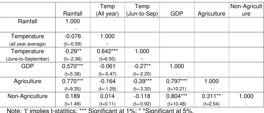
Table 1 illustrates the statistical characteristics of the processed series. The
means of all the series are almost zero and results of the Augmented Dickey-Fuller
test demonstrate that all the series are well de-trended and stationalized. The levels
of calculated volatilities are roughly similar to those in Ghate et al. (2013), which are
calculated by annual growth rates rather than HP-filtered series. June-to-September
rainfall has the highest volatilities among the five series.
Rainfall variability has a significant positive correlation with agriculture at 0.77
25
positive correlation with non-agriculture at 0.19 (t=1.49). Agriculture has a significant
positive correlation with non-agriculture at 0.31 (=2.54) and aggregate output at 0.79
(t=10.21). Non-agriculture has a positive significant correlation with aggregate output
at 0.80(t=10.48). (Table 2)
When rainfall drops below 10% of the long-term trend the situation is
categorized as a drought in the case of India (Gadgil and Gadgil, 2006). Therefore,
the impact of rainfall variability will basically be shown as the impact of a 10%
positive or negative deviation from the trend, unless otherwise stated.
4.2. Average Impact, 1952–2013
This section implements the estimation of the average impact of rainfall on
macroeconomics during the period 1952–2013 using the empirical framework
developed in section 3 and the data as set out in subsection 4.1. Pondering some
volatility decline in the examined series over time, GLS estimation will be employed
rather than OLS to address the potential concerns on heteroskedasticity. Note that
the two-stage approach does address the issue of the rapidly changing share of
agriculture and non-agriculture in total output, although the changing nature of the
parameters themselves is not addressed. The estimation basically returns the
average effects during the years 1952 to 2013.
26
Table 3. The estimated impact of rainfall variability at time t on the agricultural
production cycle at time t is significant at 1% in all specifications. The lagged rainfall
variability term is also significant at 5% on agricultural production at time t. On the
other hand, lagged agricultural production is not significant at 5%. The fitness
measured by adjusted R-squares is also high at around 60% in the specifications
including the rainfall variability term, but low in the other specification.
Turing to the magnitude of the impact, the 10% negative rainfall deviation at
time t is associated with a 3.1–3.2% negative deviation in agricultural production at
time t. This is lower than the results of Virmani (2006) at 3.6% and Gadgil and Gadgil
(2006) at 4.5%, presumably due to the addition of the recent 10 years (i.e. 2003/04–
2013 into the examined sample, where resilience to rainfall variability should have
increased due to irrigation and other developments. The 10% negative deviation of
lagged rainfall variability is associated with a 0.7% negative deviation in agricultural
production from the trend.
Given the increasing attention on the impact of temperature shocks on the
economy, a specification incorporating temperature’s deviation from its trend is also
conducted. This finds that it is significant at 1% when it is solely included but the
fitness is not high, suggesting that temperature variability has much less explanatory
27
Furthermore, this specification has significant omitted variable bias due to the
exclusion of the rainfall variability term. The temperature variability term is also
significant at 5%, when it is included with the rainfall variability term. However,
correct measurements of each parameter for rainfall and temperature can be difficult
because of multicollinearity arising from the correlation between high temperatures
and low rainfall variability in the Monsoon season (Table 2). The lower impact of
rainfall variability in the specification with temperature variability could be a result of
this multicollinearity. Based on the high explanatory power of rainfall compared with
temperature and the concerns by the multicollinearity issue, the rest of the exercise
will focus solely on the impact of rainfall variability as a representative variable for
weather shocks with respect to agricultural performance.
A comprehensive robustness check covering the whole of the two-stage
estimation will be set out later by conducting a simulation using formulated
hypothetical series to test if the estimation captures the true values of the
parameters. Here, I present only two regular robustness checks of the first-stage
estimation. The first is on the omitted variable bias. To address the concern,
specifications with the addition of inflation measured by Consumer Price Index and
Wholesale Price Index and irrigation and arable land expansions are tried. However,
28
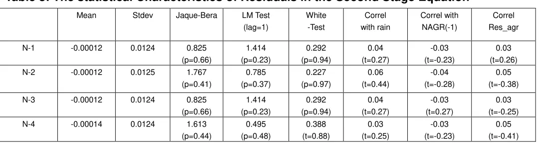
shown in order to save space. The second is a residual test. The statistical nature of
the residuals in the first-stage estimation is shown in Table 4. Their means are
almost zero. They do not correlate with the explanatory variable of rainfall deviation.
The null hypotheses of having normal distribution, homoskedasticity, and no serial
correlation are not rejected by Jarque-Bera test, the White test or the Lagrange
multiplier (LM) tests, respectively for all the specifications with the exception of the
normal distribution test for the A-3 specification – which only includes lagged
agricultural production cycle term – and is outlined in Table 3.
Based on the results of the first-stage estimation demonstrating high
explanatory power and the robustness of rainfall variability terms, the A-1 and A-2
specifications – whose explanatory variables are rainfall variability – will be chosen
to be used for the second-stage estimation from among the six specifications in
Table 3. Specifically, the second-stage exercise conducts the estimation of
Equation 17 exploiting the results of the A-1 specification and that of Equation 21
exploiting the results of A-2 specification. Furthermore, variations to account for the
changing relative weight of agriculture and non-agriculture like Equation 18 in case
of Equation 17 will also be conducted. In sum, the above mentioned four
specifications will be conducted in the second stage. Note that direct impact of
29
specification, while Equation 17 and Equation 21 account for the indirect impact of
rainfall variability at time t-1 through its impact on non-agriculture.
The estimated results of the second-stage estimation for non-agriculture are
displayed in Table 5. All of the explanatory variables, rainfall, the transmission
parameter from agriculture to non-agriculture, and the persistence of non-agriculture,
are significant at 1% and all the four specifications return very similar results.
However, the LM tests for the residual of the second-stage equation suggest
there is a possibility of serial correlation (Table 6). Therefore, the specifications of
the with-MA(1) term are also tested. The results are shown in Table 7, which cleared
the residual tests including LM tests as shown in Table 8. Note that other tests for
the residuals than LM test are cleared both in without MA(1) specification as showed
in Table 6. In specific, their means are almost zero; They do not correlate with the
explanatory variable of rainfall deviation, lagged non-agricultural production, and
agricultural unique shocks; The null hypotheses of having normal distribution and
homoskedasticity are not rejected by the Jarque-Bera test or the White test
respectively.
Rainfall variability has a significant impact on non-agriculture at the 1%
significance level. The magnitude of the impact on non-agriculture in the with-MA(1)
30
trend at time t lowers the non-agricultural production at time t by 0.46–0.53% from its
trend, which is roughly one-sixth of rainfall variability’s impact on agriculture. The
indirect impact of rainfall variability at time t, which captures the impact on
non-agriculture through rainfall’s impact on agriculture, dominates and in fact slightly
exceeds the overall impact of rainfall, ranging between 0.47% and 0.58%. The
estimation results using the without-MA(1) specification are very similar for the
overall impact and for the indirect impact in both significance and magnitude.
On the other hand, the direct impact turns out to be negative in three out of four
specifications using the with-MA(1) specifications and positive in all of the
specifications using the without-MA(1) specification as well as one of the with-MA(1)
specifications, although their magnitudes are marginal, ranging between negative
0.05% and positive 0.02% as the impact of 10% positive deviations. Therefore, the
direct impact should be judged as being marginal. In fact, the time-varying estimation
in the next subsection will show that it changes over time from negative to positive.
This is also why the signs of the direct impact of rainfall variability on non-agriculture
are sensitive to specifications as well as the reason that the magnitude of the impact
is marginal.
Based on the two-stage estimation results of rainfall’s impact on agriculture
31
the period 1952–2013 can be calculated. Using the average share of agriculture
(33%) and non-agriculture (67%) in GDP during these years, the average impact of
10% positive rainfall deviation at time t on GDP during 1952 to 2013 is positive 1.4%,
which is roughly similar to the results seen in the previous works by Virmani (2006)
and Gadgil and Gadgil (2006), which showed 1.6%. Combined with the lagged
rainfall’s impact on agriculture at 0.3%, the average overall impact during 1952 to
2013 on GDP is 1.7%.
A Further Robustness Check by Simulation. Since the two-stage estimation
framework developed in the present paper is unique, simulations are also conducted
to check if the two-stage empirical framework can estimate the unbiased true
parameters if the assumed structure is correct. Specifically, one-thousand series of
rainfall variability, agriculture business cycle, and non-agriculture business cycle are
produced, using functions of econometric software to produce random shocks
whose sizes are similar to actual data sets. Then, the two-stage estimations are
conducted to check if the true values are estimated. The results demonstrate that the
average estimated values are very close to the true values and the estimations are
valid (see the Appendix for details of the simulation).
4.3. Time-Varying Impact, 1952–2013
32
parameters are fixed during the examined period between 1952 and 2013. However,
it is natural to assume that the parameters are also time-varying. As reviewed in
section 2, the resilience of agriculture to rainfall variability should have increased
due to irrigation developments and other water management improvements, and the
transmission parameter should be changing due to dramatic changes in relative
weight of agriculture to non-agriculture. Therefore, this section will estimate
time-varying parameters by employing the Kalman filter technique following
Hamilton (1994). Based on the results seen in subsection 4.2, two basic
specifications are chosen. The first specification includes only contemporaneous
weather terms and is named the ‘without lag’ pattern. The observation equations for
the first set are below, which are modifications of Equation 15and 17:
𝐴̃𝑡 =β𝐴,𝑡𝑤̃𝑡 + 𝑒𝑡𝐴 ~𝑁𝐼𝐷(0, 𝜎𝐴) (eq.26)
𝑁̃𝑡 =β𝑁,𝑡 𝑡𝑜𝑡𝑎𝑙
𝑤̃𝑡 +ρ𝑁,𝑡𝑁̃𝑡−1+ 𝛼𝑡 𝑒𝑡𝑎+ 𝑒𝑡𝑛~𝑁𝐼𝐷(0, 𝜎𝑁) (eq.27)
The state equations are below:
β
𝐴,𝑡+1 =β𝐴,𝑡+ 𝑣𝑡𝐴~𝑁𝐼𝐷(0, 𝜎𝑣𝐴) (eq.28)
β 𝑁,𝑡+1 𝑡𝑜𝑡𝑎𝑙
= β
𝑁,𝑡 𝑡𝑜𝑡𝑎𝑙
+ 𝑣𝑡𝑁~𝑁𝐼𝐷(0, 𝜎𝑣𝑁)(NID) (eq.30)
ρ
𝑁,𝑡+1 =ρ𝑁,𝑡+ 𝑣𝑡
𝜌~𝑁𝐼𝐷(0, 𝜎𝜌)(NID) (eq.31)
α
𝑡+1= α𝑡 + 𝑣𝑡𝛼~𝑁𝐼𝐷(0, 𝜎𝛼)(NID) (eq.32)
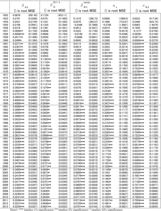
33
𝐴̃𝑡 = β𝐴,𝑡 𝑇
𝑤̃𝑡 +β𝐴,𝑡 𝑇−1
𝑤̃𝑡−1+ 𝑒𝑡𝐴~𝑁𝐼𝐷(0, 𝜎𝐴 ′
)(𝑖. 𝑖. 𝑑) (eq.33)
𝑁̃𝑡 = β𝑁,𝑡 𝑡𝑜𝑡𝑎𝑙
𝑤̃𝑡 +ρ𝑁,𝑡𝑁̃𝑡−1+ 𝛼𝑡 (β𝐴 𝑇−1
𝑤̃𝑡−1+ 𝑒𝑡𝑎) + 𝑒𝑡𝑛~𝑁𝐼𝐷(0, 𝜎𝑁 ′
) (eq.34)
The state equations are the same for ρ
𝑁,𝑡, β𝑁,𝑡
𝑡𝑜𝑡𝑎𝑙
and 𝛼𝑡 , and those for β 𝐴,𝑡 𝑇
and β 𝐴,𝑡 𝑇−1
are as follows:
β 𝐴,𝑡+1 𝑇
=β
𝐴,𝑡 𝑇
+ 𝑣𝑡𝐴,𝑇~𝑁𝐼𝐷(0, 𝜎𝑣𝐴′) (eq.35)
β 𝐴,𝑡+1 𝑇−1
=β
𝐴,𝑡 𝑇−1
+ 𝑣𝑡𝐴,𝑇−1~𝑁𝐼𝐷(0, 𝜎𝑣𝐴") (eq.36)
The decomposition of overall impact on non-agriculture to direct and indirect impacts,
and the aggregation to get the overall impact, follows the same procedure as was
undertaken in subsection 4.2. Note that the accounting changing relative weight of
agriculture to non-agriculture is no more needed (as done in subsection 4.2)
because the parameters themselves are allowed to alter this subsection’s excercise.
Note also that the MA(1) term is not added in the second-stage estimation for
non-agriculture in order to simplify the estimation. This is allowable, given that the
results for the overall estimation for rainfall variability term were similar in the
previous subsection’s exercise.
Following the standard procedure, the sizes of innovation variance terms (i.e.
𝜎), which minimize the prediction errors for parameters are estimated by maximum
likelihood estimation . The results, especially the trends of parameters over time, are
34
generally higher than those of the GLS estimation in the previous section as will be
shown later, suggesting there is a possibility of overestimation. Therefore, larger
sizes of innovation variance, which keep the significance at 5% for the parameter
estimation, rather than the size of innovation variance estimated by standard
procedures, are also tried to assess the susceptibility of results to the innovation size
for reference purposes. Note that larger innovation variation enables us to follow the
changes in parameters more quickly and vividly. For convenience, the estimation
with the larger innovation variance is named the ‘flex’ pattern, and those using the
standard procedure are termed the ‘steady’ pattern in this paper.
In sum, the following four specifications will be tried: ‘steady without lag’, ‘flex
without lag’, ‘steady with lag’, and ‘flex with lag’. The results will be shown for each
category of rainfall variability’s impacts on agriculture, non-agriculture and then
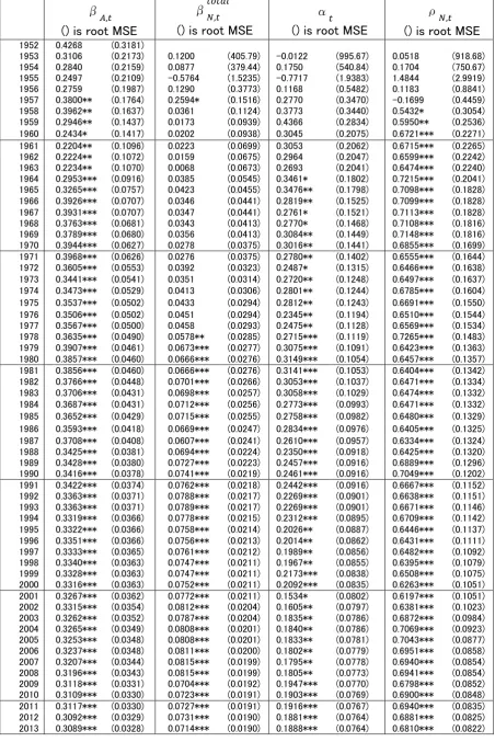
those on GDP in figures 1 to 8. In the figures, the results between 1965 and 2013
are shown as the results before 1965 are volatile (i.e. taking some to converge to
plausible results), as is often seen when employing a Kalman filter estimation. The
comprehensive estimated results are shown only for steady patterns in Table 9 and
Table 10, while those for flex patterns, which are conducted for reference purpose,
are not shown to save space.
35
variability on agricultural production are demonstrated in Figure 1. All four patterns
demonstrate that the impacts of 10% positive rainfall deviations are elevated to a
high of roughly 4% in the late 1970s to early 1980s, and then decline thereafter. The
speed of the decline in the flex patterns is faster than that of the steady patterns, as
would be expected. The impacts drop to 2% in recent years in the case of the flex
pattern, while the steady pattern remains higher at 3% in recent years. The impact of
the previous year’s rainfall shock (i.e. 10% positive deviation) on agricultural
production has continuously decreased from roughly 1.0% to 0.7% in all of the four
patterns. This decline in rainfall’s impact on agriculture over time is consistent with
the findings of Gadgil and Gadgil (2006).
The fluctuations of the above rainfall impacts on agriculture can be interpreted
consistently with India’s agricultural developments. What follows is a chronological
interpretation of such a circumstance. The lower sensitivity to rainfall shocks in the
early 1960s can be associated with a massive expansion of sown areas. The
expansion of cropland was sustained at a high pace in the 1950s and the early
1960s, and the agricultural production increase prior to the early 1960s was largely
due to the expansion in sown areas (Singh, 2000). Thus, additional production in
newly cultivated areas may have alleviated or sometimes negated the negative
36
agricultural strategy of adopting high yielding variety (HYV) seeds, chemical
fertilizers, and irrigation facilities called the ‘Green Revolution’ was implemented to
achieve self-sufficiency in food grain (ibid). Since HYV seeds’ production
performance is susceptive to water conditions, sensitivity to rainfall variability surged
and remained high with the increased use of HYV seeds in the late 1960s and 1970s.
From the early 1980s, however, susceptibility to rainfall variability decreased steadily
as the benefits from the continuous increase in irrigated croplands from the 1970s to
the 1990s became visible, overwhelming the increased susceptibility to water
conditions due to the increased use of HYV seeds. Agricultural investment is known
to have dropped in the early to mid-1980s, due to the decline in public investment
resulting from the deterioration in fiscal conditions, but started picking up in the late
1980s and 1990s due to the in surge private investment (Gulati and Bathla, 2001).
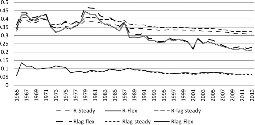
Non-Agriculture. The overall impact of rainfall variability on non-agriculture in all the
four patterns are similar in trends. The overall impact started to increase in the early
1970s and accelerated in the late 1970s. It continued to increase at a slow pace until
the mid-2000s, then dropped in 2009 and has remained at a lowered level until in
early 2010s. Focusing on the steady pattern, the detailed results are as follows. The
overall impact of 10% positive deviations increases rapidly from a low of 0.4% in the
37
dropping to 0.7% in 2009 (Figure 4). The positive overall impact of rainfall variability
is supported by the sustained high indirect impacts (i.e. the impact on
non-agriculture through rainfall’s impact on agriculture) marked at roughly above
1.0% in the 1970s and 1980s, which decline steadily after the 1990s reaching below
0.6% in the 2000s and early 2010s (Figure 5). The indirect impact’s decrease is also
supported by a continuous decline of the transmission parameter as it is the impact
on agriculture multiplied by the transmission parameter (Figure 2). On the other
hand, the direct impact of the 10% positive rainfall deviation steadily increased from
the negative values at below negative 0.5% in the 1960s, turning positive in the early
1990s and reaching 0.3% in the 2000s, with a drop to 0.2% in the early 2010s
(Figure 6).
There are two key points in the above results. Firstly, the pattern of the direct
impact on non-agriculture lags behind the impact on agriculture and indirect impact
on non-agriculture by almost two to three decades. This lag can be associated with
the slow belief formation process of Indian people in regard to the impact of rainfall
on the economy, which will be discussed further in the next subsection. Secondly,
the direct impact on non-agriculture changed from negative values in the 1960s to
1980s to positive values in the 1990s to 2010s. The negative value can be
38
country. An interpretation of the positive direct impact will be discussed further in the
next subsection, as it is not straightforward.
The Aggregate Impacts on GDP. The overall impacts of rainfall variability on
GDP can be obtained by aggregating the results on agriculture and non-agriculture
by their respective share in GDP. Figure 7 demonstrates the results for the steady
pattern without lag and Figure 8 for the steady pattern with lag. The results vividly
depict the dynamism of the changes in the weather–economy relationship. The key
chronological stories that the aggregated results reflect are as follows. The direct
impact on agriculture and its transmission to non-agriculture grew in the 1960s and
remained high until the late 1970s, and declined thereafter. Despite the reduced
share of agriculture in GDP since the 1980s, agriculture-related impacts of rainfall
variability dominate rainfall variability’s impact on the economy as a whole
throughout the examined period. On the other hand, the direct impact of rainfall
variability on non-agriculture was negative until the 1980s, being vulnerable to
natural disasters due to underdeveloped infrastructure. The direct impact on
non-agriculture becomes positive in the 1990s and remains so thereafter. In sum
then, the impact on non-agriculture is confirmed but a large part of it is rooted in
agriculture-related impacts.
39
This subsection discusses three issues, which are associated with the previous
subsection’s results on the time-varying impacts.
4.4.1 The Positive Direct Impact on Non-Agriculture and People’s Beliefs
The interpretation of a ‘positive’ direct impact of rainfall variability on non-agriculture
is difficult compared with the more straightforward interpretation of negative shocks
as a result of natural disasters and underdeveloped infrastructure. The increase of
resilience to rainfall shocks through infrastructure development at a maximum only
explains changes from negative values to zero. Moreover, it is also not
straightforward compared with the indirect impact of rainfall on non-agriculture,
which can be considered a natural result of the strong linkage between agriculture
and non-agriculture in India.
One of the candidates to explain the positive direct impact is the impacts of
rainfall variability information on people’s expectations. If people expect good
economic performance due to positive rainfall shocks, people may consume and
produce more when they see the rainfall shocks. For instance, farmers may
consume more in anticipation of future increased income, and non-farm employers
produce more due to them expecting more consumption by farmers. The crucial
nature of rainfall that it is visible to all people, a fact further augmented by the
40 on people’s expectations can be strong.
If the direct positive impacts are due to people’s expectations, the direct impact
can be considered a kind of error arising from the difference between expectations
formed by information on rainfall precipitation and its actual impact on agriculture
and non-agriculture. This is consistent with the results that indirect impact is much
larger than the direct impact. Note that indirect impact captures the impact of ‘actual’
agricultural production on non-agriculture, while other factors related to weather
shocks such as the impact of rainfall variability on people’s expectations are not
necessarily captured as the indirect impact as understood from the structure of
Equation 16.
If the direct positive impact on non-agriculture is associated with the rainfall
shock’s impact on people’s expectations, how can we interpret the lagged peak of
the direct impact compared with that of indirect impact? The indirect impacts peak in
the late 1970s and early 1980s, while the direct impact continued to improve to reach
a peak in the mid-2000s. Furthermore, the increase of the direct impact in the 1980s,
1990s and early 2000s occurred when the indirect impacts declined continuously.
The lagged peak could be associated with the notions that people’s beliefs
change slowly. People expects based on their belief on how rainfall variability affects
41
rainfall performance in Ethiopia and Kenya, argued that people’s beliefs take time to
alter, even if they are exposed to new information and especially when that new
information is ambiguous. This is called confirmation bias. In the case of India, it is
natural to assume that people’s beliefs were built slowly and steadily through
people’s experience of an economy in which agriculture’s share was high and where
the linkage between agriculture and non-agricultural production was growing, such
as was seen in the 1970s and 1980s. However, it takes time for people to update
their beliefs because assessing the extent of the influence of a reducing agricultural
share is difficult for most individuals. Indeed, new information on the reduced share
of agriculture in the economy is ambiguous in the sense that how far people should
take account of it to make economic decisions is not clear. It is worth recalling that
agriculture’s impact on non-agricultural production is real for people, even if people
recognize the declining importance of agriculture in the economy. If people react to
rainfall information based on past experience or old information, the economy may
overreact to rain fluctuations and the Monsoon’s impact can remain high compared
with the real production structure.
4.4.2 The Impact of Temperature on Non-Agriculture
The second candidate to explain the positive direct impact of rainfall shocks on
42
temperature shocks. In India, a precipitation shock is negatively correlated with a
temperature shock in the Monsoon season (Table 2). Therefore, the positive impact
of positive rainfall shocks could be a result of the negative temperature shocks such
as increase in productivity or decrease in mortality (Dell.et al. 2014)
The negative impact of high temperatures on the economy is a plausible
hypothesis. However, Figure 9, which illustrates the residuals of the AR1 estimation
for non-agriculture’s cyclical component and temperature shocks (i.e. temperature
for the all-year average de-trended by the HP filter), raises some difficulties in terms
of adopting and even examining the hypothesis. The relationship between
temperature shocks and non-agriculture’s performance is roughly negative in the
pre-1991 reform period, but roughly positive after the 1991 reform. Thus, there
emerges the possibility that a high temperature shock can be associated with high
growth.
Here, the second-stage equation (Equation 17) will be extended as below to
include the temperature shock in order to directly examine if it has a positive
relationship in the post-1991 reform period:
𝑁̃𝑡 =
β 𝑁,𝑡 𝑡𝑜𝑡𝑎𝑙
β 𝑁 𝑡𝑜𝑡𝑎𝑙
𝑤̃𝑡 +ρ𝑁𝑁̃𝑡−1+ 𝛼 𝑒𝑡𝐴+β𝑛
𝑡𝑒𝑚𝑝1990
∗ 𝑑𝑢𝑚𝑚𝑦1990 ∗ 𝑇̃𝑡 +
β 𝑛
𝑡𝑒𝑚𝑝1991
∗ 𝑑𝑢𝑚𝑚𝑦1991 ∗ 𝑇̃𝑡 + +𝑒𝑡𝑁 (eq.37)
43
‘dummy1991’ are standard dummies being composed of zeros and ones. β 𝑛
𝑡𝑒𝑚𝑝1990
captures the impact of a temperature shock on non-agriculture’s performance until
1990, and β 𝑛
𝑡𝑒𝑚 �1990
captures it after 1991. Unlike the exercise done for the
impacts of temperature shocks on agriculture, the all-year average temperature
shocks rather than June-to-September temperature shock will be basic case to
match the purpose of the exercise as well as to avoid multicollinearity arising from
the negative correlation between rainfall deviation and temperature in the Monsoon
season. Furthermore, to address the serial correlation issue, the specification with
MA1 is also included. The estimation is done by OLS for the with-MA1 specification
and by GLS for the without-MA1 specification using data from the entire period, 1952
to 2013.
The estimation results are shown in Table 11 and residual test results are
shown in Table 12. The residual shock tests and the abovementioned
multicollinearity issue suggests that the T-1 specification with the all-year average
temperature and MA1 term is the most reliable result. As expected from the figure, it
shows that temperature shock and non-agricultural performance had a negative
relationship until 1990, which is consistent with the hypothesis of the negative shock
of high temperature represented by a decrease in labor productivity, although it