Generalized geometric quantum speed limits

Generalized Geometric Quantum Speed Limits

Diego Paiva Pires,1,*Marco Cianciaruso,2,3,4,† Lucas C. Céleri,5,‡ Gerardo Adesso,2,§ and Diogo O. Soares-Pinto1,∥ 1_{Instituto de Física de São Carlos, Universidade de São Paulo,}

CP 369, 13560-970 São Carlos, São Paulo, Brazil

2_{School of Mathematical Sciences, The University of Nottingham, University Park,} Nottingham NG7 2RD, United Kingdom

3_{Dipartimento di Fisica“E. R. Caianiello,”Università degli Studi di Salerno,} Via Giovanni Paolo II, I-84084 Fisciano (SA), Italy

4_{INFN, Sezione di Napoli, Gruppo Collegato di Salerno, I-84084 Fisciano (SA), Italy} 5

Instituto de Física, Universidade Federal de Goiás, 74.001-970 Goiânia, Goiás, Brazil

(Received 21 July 2015; revised manuscript received 11 March 2016; published 2 June 2016)

The attempt to gain a theoretical understanding of the concept of time in quantum mechanics has triggered significant progress towards the search for faster and more efficient quantum technologies. One of such advances consists in the interpretation of the time-energy uncertainty relations as lower bounds for the minimal evolution time between two distinguishable states of a quantum system, also known as quantum speed limits. We investigate how the nonuniqueness of a bona fide measure of distinguishability defined on the quantum-state space affects the quantum speed limits and can be exploited in order to derive improved bounds. Specifically, we establish an infinite family of quantum speed limits valid for unitary and nonunitary evolutions, based on an elegant information geometric formalism. Our work unifies and generalizes existing results on quantum speed limits and provides instances of novel bounds that are tighter than any established one based on the conventional quantum Fisher information. We illustrate our findings with relevant examples, demonstrating the importance of choosing different information metrics for open system dynamics, as well as clarifying the roles of classical populations versus quantum coherences, in the determination and saturation of the speed limits. Our results can find applications in the optimization and control of quantum technologies such as quantum computation and metrology, and might provide new insights in fundamental investigations of quantum thermodynamics.

DOI:10.1103/PhysRevX.6.021031 Subject Areas: Quantum Physics, Quantum Information

I. INTRODUCTION

Quantum mechanics relies on counterintuitive features that challenge our merely classical perception of nature. One of the most fundamental quantum aspects lies in the impossibility of knowing simultaneously and with certainty two incompatible properties of a quantum system [1]. Contrarily to the well-understood uncertainty relation between any two noncommuting observables, the time-energy uncertainty relation still represents a controversial issue [2], although the last decades witnessed several attempts towards its explanation [3]. This effort led to the interpretation of the time-energy uncertainty relation as a so-called quantum speed limit (QSL), i.e., the ultimate

bound imposed by quantum mechanics on the minimal evolution time between two distinguishable states of a system [4–41]. QSLs have been widely investigated within the quantum-information setting since their understanding offers a route to design faster and optimized information-processing devices [42], thus attracting constant interest in quantum optimal control, quantum metrology [43], and quantum computation and communication[44]. Interestingly, it has been recently recognized that QSLs also play a fundamental role in quantum thermodynamics[45].

In a seminal work, Mandelstam and Tamm (MT) [4] reported a QSL for a quantum system that evolves between two distinguishable pure states, jψð0Þi and jψðτÞi, via a unitary dynamics generated by a time-independent HamiltonianH. The ensuing lower bound on the evolution time is given by τ≥ℏarccosðjhψðτÞjψð0ÞijÞ=ΔE, where ðΔEÞ2¼ hH2i−hHi2 is the variance of the energy of the system with respect to the initial state. Several years later, Anandan and Aharanov[7]extended the MT bound to time-dependent Hamiltonians by using a geometric approach that exploits the Fubini-Study metric defined on the space of quantum pure states. Specifically, they simply used the fact that the geodesic length between two distinguishable pure states according to the Fubini-Study *_{[email protected]}

†_{[email protected]} ‡_{[email protected]}

§

[email protected]

∥_{[email protected]}

metric, i.e., their Bures angle, is a lower bound to the length of any path connecting the same states. Over half a century after the MT result, Margolus and Levitin (ML) [16] provided a different QSL on the time evolution of a closed system whose Hamiltonian is time independent and evolv-ing between two orthogonal pure states. This bound reads as τ≥πℏ=ð2EÞ, where E¼ hHi is the mean energy. Although the ML bound is tight, it does not recover the MT one whatsoever. Therefore, the quantum speed limit for unitary dynamics, when restricting to orthogonal pure states, can be made tighter by combining these two independent results asτ≥maxfπℏ=ð2ΔEÞ;πℏ=ð2EÞg[17].

All these results attracted considerable interest in the subject. Giovannettiet al.[18]extended the ML QSL to the case of arbitrary mixed states and also showed that entanglement can speed up the dynamical evolution of a closed composite system. A plethora of other extensions and applications of QSLs for unitary processes has been investigated in Refs. [5,6,8–15,19–30]. For example, in Ref. [29] some of us show that the rate of change of the distinguishability between the initial and the evolved state of a closed quantum system can provide a lower bound for an indicator of quantum coherence based on the Wigner-Yanase information between the evolved state and the Hamiltonian generating the evolution.

Since any information-processing device is inevitably subject to environmental noise, QSLs have also been investigated in the nonunitary realm. Taddei et al. [31] and del Campoet al.[32]were the first to extend the MT bound to any physical process, whether it was unitary or not. Specifically, Ref. [31] exploits the quantum Fisher information metric on the whole quantum state space and represents a natural extension of the idea used in Ref.[7], whereas Ref.[32]exploits the relative purity. Then, Deffner and Lutz [33] extended the ML bound to open quantum systems by adopting again a geometric approach using the Bures angle. These authors have also introduced a new sort of bound, which is tighter than both the ML and MT ones, and shown that non-Markovianity can speed up the quantum evolution. Some other works then provided a QSL for open system dynamics by using the relative purity, whose usefulness ranges from thermalization phenomena [34] to the relativistic effects on the QSL [35]. Further developments include the role of entanglement in QSL for open dynamics [36–38], QSL in the one-dimensional perfect quantum state transfer [44], and the experimental realizability of measuring QSLs through interferometry devices [39]. Finally, a subtle connection was recently highlighted between QSLs and the maximum interaction speed in quantum spin systems[40], with implications for quantum error correction and the relaxation time of many-body systems [41].

Distinguishing between two states of a system being described by a probabilistic model stands as the paradig-matic task of information theory. Information geometry, in

particular, applies methods of differential geometry in order to achieve this task[46]. The set of states of both classical and quantum systems is indeed a Riemannian manifold, that is, the set of probability distributions over the system phase space and the set of density operators over the system Hilbert space, respectively. Therefore, it seems natural to use any of the possible Riemannian metrics defined on such sets of states in order to distinguish any two of its points. However, it is also natural to assume that for a Riemannian metric to be bona fide in quantifying the distinguishability between two states, it must be contractive under the physical maps that represent the mathematical counterpart of noise, i.e., stochastic maps in the classical settings and completely positive trace-preserving maps in quantum. Interestingly, Čencov’s theorem states that the Fisher information metric is the only Riemannian metric on the set of probability distributions that is contractive under stochastic maps[47], thus leaving us with only one choice of bona fide Riemannian geometric measure of distinguish-ability within the classical setting. On the contrary, it turns out that the quantum Fisher information metric[48,49]is not the only contractive Riemannian metric on the set of density operators, but rather there exists an infinite family of such metrics [50], as characterized by the Morozova, Čencov, and Petz theorem[51,52].

In this paper, we construct a new fundamental family of geometric QSLs (see Fig. 1), which is in one-to-one correspondence with the family of contractive Riemannian metrics characterized by the Morozova,Čencov, and Petz theorem. We demonstrate how such nonuniqueness of a bona fide measure of distinguishability defined on the quantum-state space affects the QSLs and can be exploited in order to look for tighter bounds. Our approach is versatile enough to provide a unified picture, encompassing both unitary and nonunitary dynamics, and is easy to handle, requiring solely the spectral decomposition of the evolved state. This family of bounds is naturally tailored to the general case of initial mixed states and clearly separates the contribution of the populations of the evolved state and the coherences of its time variation, thus clarifying their individual roles in driving the evolution.

The paper is organized as follows. In Sec.II, we review the relation between statistical distinguishability and the contractive Riemannian metrics on the quantum-state space characterized by the Morozova,Čencov, and Petz theorem. SectionIIIprovides a new generalized geometric derivation of a family of QSLs, which is in one-to-one correspondence with the family of such metrics. In Sec. IV, we illustrate and compare the obtained bounds for both unitary and nonunitary evolutions. Finally, in Sec. V, we present our conclusions.

II. GEOMETRIC MEASURES OF DISTINGUISHABILITY

According to the standard formulation of quantum mechanics, any quantum system is associated with a Hilbert space H and its states are represented by the Riemannian manifoldS¼DðHÞof density operators over

H, i.e., the set of positive semidefinite and trace-one

operators over the carrier Hilbert space. A Riemannian metric overSis said to be contractive if the corresponding geodesic distanceLcontracts under physical maps, which means it satisfies the inequality LðΛðρÞ;ΛðσÞÞ≤Lðρ;σÞ

for any completely positive trace-preserving map Λ and any ρ;σ∈S. The Morozova, Čencov, and Petz theorem provides us with a characterization of such metrics in the finite-dimensional case, by constructing a one-to-one correspondence between them and the Morozova-Čencov (MC) functions, a function fðtÞ∶R_þ→R_þ which is (i) operator monotone: for any semipositive-definite oper-atorsAandBsuch thatA≤B, thenfðAÞ≤fðBÞ; (ii)

self-inversive: it fulfills the functional equationfðtÞ ¼tfð1=tÞ;

and (iii) normalized:fð1Þ ¼1. Specifically, the Morozova, Čencov, and Petz theorem states that every contractive Riemannian metricgfassigns, up to a constant factor, the following squared infinitesimal length between two neigh-boring density operatorsρandρþdρ[53]:

ds2≔gf_ρðdρ; dρÞ; ð1Þ

with

gf

ρðA; BÞ ¼1

4Tr½AcfðLρ;RρÞB; ð2Þ

whereAandBare any two traceless Hermitian operators, and

cf_{ðx; yÞ≔} 1

yfðx=yÞ ð3Þ

is a symmetric function,cf_{ðx; yÞ ¼c}f_{ðy; xÞ, which fulfills}

cf_{ðαx;αyÞ ¼α}−1_cf_{ðx; yÞ, withfðtÞbeing a MC function,}

and finally L_ρ;R_ρ∶BðHÞ→BðHÞ are two linear super-operators defined on the setBðHÞof linear operators over

Has follows:L_ρA¼ρAandR_ρA¼Aρ. We stress again that each contractive Riemannian metric is arbitrary up to a constant factor. In accordance with Ref. [54], we have chosen the factor1=4in order to make the entire family of contractive Riemannian metrics collapse to the classical Fisher information metric whenρand dρcommute.

In order to make Eq. (1) more explicit, we can write the density operator ρ in its spectral decomposition, ρ¼Pjpjjjihjj, with 0< pj≤1 and

P

jpj¼1, and

get[54]

ds2¼1

4

X

j

ðdρjjÞ2

p_j þ2

X

j<l

cf_ðp

j; plÞjdρjlj2

; ð4Þ

wheredρ_jl≔hjjdρjli, and we note that the summation is

constrained to the requirement pj>0. Equation (4) is

crucial since it clearly identifies two separate contributions to any contractive Riemannian metric. The first term, which is common to all the family, depends only on the

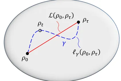
FIG. 1. Illustration of geometric quantum speed limits. The dashed blue curve is the path γ in the quantum-state space representing a generic evolution between an initial stateρ₀and a final stateρτ, parametrized by timet∈½0;τ. Given a metric on the quantum-state space, the length of this path is denoted by

lγðρ0;ρτÞ. The solid red curve denotes the geodesic connecting

ρ0 to ρτ, whose length is given by Lðρ0;ρτÞ. Quantum speed limits originate from the fact that the geodesic amounts to the path of shortest length among all physical evolutions between the given initial and final states: Lðρ₀;ρτÞ≤lγðρ₀;ρτÞ∀γ. Such inequality can be interpreted as follows. For any given physical evolutionγfromρ₀toρτ, and according to any valid metric, the maximum distance between the initial ρ₀ and the final state

populationspjofρand can be seen as the classical Fisher

information metric at the probability distribution p_j. The second term, which is responsible for the nonuniqueness of a contractive Riemmanian metric on the quantum-state space, is instead only due to the coherences of dρ with respect to the eigenbasis of ρ and is a purely quantum contribution expressing the noncommutativity between the operators ρ and ρþdρ. Finally, for all the contractive Riemannian metrics that can be naturally extended to the boundary of pure states, such that fð0Þ≠0, the Fubini-Study metric always appears to be such an extension up to a constant factor, so the nonuniqueness of a contractive Riemannian geometry can only be witnessed when con-sidering quantum mixed states. This is the reason only the mixed states will be relevant in our analysis, whose aim is exactly to investigate the freedom in the choice of several inequivalent bona fide measures of indistinguishability in order to get tighter QSLs.

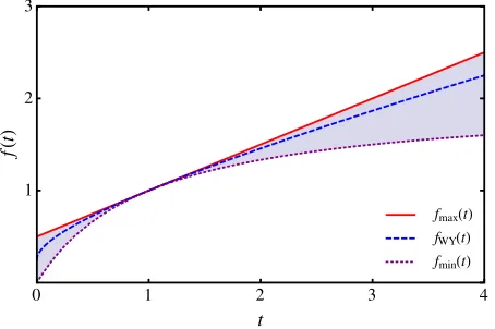
As pointed out by Kubo and Ando[55], among the MC functions, there exists a minimal one,fminðtÞ ¼2t=ð1þtÞ,

and a maximal one, fmaxðtÞ ¼ ð1þtÞ=2, such that a

generic MC function fðtÞ must satisfy fminðtÞ≤fðtÞ≤ f_maxðtÞ. Interestingly, the maximal MC function is the one

corresponding to the celebrated quantum Fisher informa-tion metric, whereas the Wigner-Yanase informainforma-tion metric corresponds to an intermediate MC function, fWYðtÞ ¼

ð1=4Þðpffiffitþ1Þ2, as illustrated in Fig.2.

Each of these metrics plays a fundamental role in quantum information theory since the corresponding geo-desic length L, being, by construction, contractive under

quantum stochastic maps, represents a bona fide measure of distinguishability over the quantum-state space. However, finding such geodesic distance is unfortunately a very hard task in general. In fact, analytic expressions are known only for the geodesic distance related to the quantum Fisher information metric[56],

LQF_{ðρ;σÞ ¼arccos½}p_Fffiffiffiffiffiffiffiffiffiffiffiffiffiffiffi_{ðρ;σÞ; ð5Þ}

whereFðρ;σÞ ¼ ðTr½ppffiffiffiffiffiffiffiffiffiffiffiffiffiffiffiffiρffiffiffiσpffiffiffiρÞ2is the Uhlmann fidelity, and for the one related to the Wigner-Yanase information metric [50],

LWY_{ðρ;σÞ ¼arccos½Aðρ;σÞ; ð6Þ}

whereAðρ;σÞ ¼TrðpffiffiffiρpffiffiffiσÞis known as quantum affinity.

III. GENERALIZED GEOMETRIC QUANTUM SPEED LIMITS

We are now ready to present our main result, that is, a family of geometric QSLs that hold for any physical process and are in one-to-one correspondence with the contractive Riemannian metrics defined on the set of quantum states. The most general dynamical evolution of an initial state ρ0 can be written in the Kraus decom-position as ρ_λ¼E_λ½ρ₀ ¼P_jK_jλρ₀Kλ_j†, where fKλ_jg are operators satisfyingP_jKλ_j†Kλ_j¼Iand depending on a set λ¼ fλ1;λ2;…;λrg of r parameters that are encoded into

the input stateρ0, in such a way thatρλdepends analytically on each parameterλ_μ(μ¼1;…; r). In the unitary case, the evolution is given, in particular, by E_λ½ρ₀ ¼U_λρ₀U†_λ, whereU_λ is a multiparameter family of unitary operators, fulfillingU_λU†_λ¼U†_λU_λ¼I. In this case, the observables

Hλ_μ¼−iℏU_λ∂_μU†_λ, with ∂_μ≡ ∂=∂λ_μ, are the generators driving the dynamics.

Consider a dynamical evolution ρ_λ in which the set of parameters λ is changed analytically from the initial configuration λI to the final one λF. Geometrically, this

evolution draws a path γ in the quantum-state space connectingρλI and ρλF whose length is given by the line integrallfγ ¼R_γds and depends on the chosen metricgf

(see Fig.1). Sinceγis an arbitrary path betweenρλIandρλF, its length need not be the shortest one, which is instead given by the geodesic lengthLf_ðρ

λI;ρλFÞbetweenρλI and ρλF. Therefore, the latter represents a lower bound for the length of the path drawn by the above dynamical evolution. This observation will play a crucial role in the imminent derivation of our family of QSLs, in analogy with Refs.[7] and[31].

Since the density operator ρ_λ evolves analytically with respect to the parametersλ, we can write

fmaxt

fWYt

fmint

0 1 2 3 4

1 2 3

t

f

t

FIG. 2. The family of MC functions is upper bounded by a maximal one, fmaxðtÞ ¼ ð1þtÞ=2, corresponding to the

quan-tum Fisher information metric (red solid line), and lower bounded by a minimal one,fminðtÞ ¼2t=ð1þtÞ(purple dotted line). Any

MC functionfðtÞsatisfiesfminðtÞ≤fðtÞ≤fmaxðtÞ; i.e., its graph

falls into the shaded area, as shown in the particular case of the MC functionfWYðtÞ ¼ ð1=4Þð

ffiffi

t

p

dρ_λ ¼X

r

μ¼1

∂μρλdλμ: ð7Þ

Letρ_λ¼P_jp_jjjihjj be the spectral decomposition ofρ_λ, with 0< pj≤1 and

P

jpj¼1. We note that both the

eigenvaluespjand eigenstatesjjiofρλmay depend on the

set of parametersλ, i.e.,pj≡pjðλÞandjji≡jjðλÞi, so that

∂μρλ¼

X

j

fð∂μpjÞjjihjj þpj½ð∂μjjiÞhjj þ jjið∂μhjjÞg;

ð8Þ

and thus

hjj∂_μρ_λjli ¼δ_jl∂_μp_jþ ðp_l−p_jÞhjj∂_μjli; ð9Þ

where we used the identity ð∂_μhjjÞjli ¼−hjj∂_μjli.

Combining Eqs. (7)and(9), we get

hjjdρλjli ¼X

r

μ¼1

½δjl∂μpjþiðpj−plÞAμjldλμ; ð10Þ

where we defineAμ_jl≡ihjj∂_μjli. By using Eq.(10), in the case of j¼l we get

jhjjdρ_λjjij2¼ X

r

μ;ν¼1

∂μpj∂νpjdλμdλν; ð11Þ

whereas in the case ofj≠l, by using the fact that dρ_λ is Hermitian, we obtain

jhjjdρλjlij2¼ X

r

μ;ν¼1

ðpj−plÞ2AjlμAνljdλμdλν: ð12Þ

Finally, by substituting Eqs.(11)and(12)into Eq.(4), the squared infinitesimal length ds2 betweenρ_λ andρ_λþdρ_λ

according to any contractive Riemannian metric gf

becomes

ds2¼ X

r

μ;ν¼1

gfμνdλμdλν; ð13Þ

where

gfμν¼FμνþQfμν; ð14Þ

with

Fμν ¼1₄

X

j

∂μpj∂νpj

p_j ; ð15Þ

and

Qf

μν¼1 2

X

j<l

cf_ðp

j; plÞðpj−plÞ2AμjlAνlj; ð16Þ

referring to, respectively, the contribution of the popula-tions ofρλ and of the coherences ofdρλ to the contractive Riemannian metric tensorgfμν. Herein, we restrict ourselves to the case where the parameters λ are time dependent, λμ¼λμðtÞ, forμ¼1;…; r, and choose the parametrization

t∈½0;τ→λðtÞ such that λI ¼λð0Þ and λF ¼λðτÞ,

where τ is the evolution time. Now, since the geodesic distanceLf_ðρ

0;ρτÞbetween the initial stateρ0and the final stateρ_τ defines a lower bound to the lengthlfγ of the pathγ followed by the evolved stateρtwhen going fromρ0toρτ,

we have

Lf_ðρ

0;ρτÞ≤lfγðρ0;ρτÞ; ð17Þ

where

lf

γðρ0;ρτÞ≔

Z _τ

0

ds dt

dt¼ Z _τ

0 dt

ffiffiffiffiffiffiffiffiffiffiffiffiffiffiffiffiffiffiffiffiffiffiffiffiffiffiffiffiffiffi Xr

μ;ν¼1

gfμνdλμ

dt dλν

dt v

u u

t :

ð18Þ

Equation (17) represents the anticipated infinite family of generalized geometric QSLs and is the central result of this paper. Any possible contractive Riemannian metricgf

on the quantum-state space, and so any possible bona fide geometric quantifier of distinguishability between quantum states, gives rise to a different QSL. More precisely, we have that both the geodesic distance appearing in the left-hand side and the quantitylfγðρ0;ρτÞin the right-hand side of Eq.(17)depend on the chosen contractive Riemannian metric, specified by a MC function f. In particular, by restricting to the celebrated quantum Fisher information metric, we recover the QSL introduced in Ref.[31].

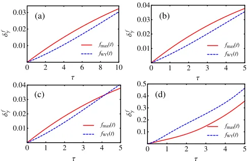
It is intuitively clear that the contractive Riemannian metric whose geodesic is most tailored to the given dynamical evolution is the one that gives rise to the tightest lower bound to the evolution time as expressed in Eq.(17). In order to determine how much a certain geometric QSL is saturated, i.e., itstightness, we consider the relative difference

δf

γ ≔l

f

γðρ0;ρτÞ−Lf_ðρ0;ρτÞ

Lf_ðρ0;ρτÞ ; ð19Þ

which quantifies how much the dynamical evolution γ differs from a geodesic with respect to the considered metric gf_.

dynamicsγ. Formally, labeling byf⋆_γ the optimal metric for the dynamics γ, the tightest possible geometric QSL is therefore defined by

Lf⋆γðρ

0;ρτÞ≤lf ⋆

γ

γ ðρ0;ρτÞ; with f⋆γ such that inf

f δ f

γ ≡δf ⋆

γ

γ ;

ð20Þ

where the minimization is over all MC functionsf. Finding this minimum is, however, a formidable prob-lem, which is made all the more difficult by the fact that the quantum Fisher information metric and the Wigner-Yanase information metric are the only contractive Riemannian metrics whose geodesic lengths are analytically known for general dynamics (as previously remarked).

Nevertheless, in this paper, we move the first steps forward towards addressing such a general problem, by restricting the optimization in Eq.(20)primarily over these two paradigmatic and physically significant examples of contractive Riemannian metrics, namely, the quantum Fisher information and the Wigner-Yanase skew informa-tion. Quite remarkably, this restriction will be enough to reveal how the choice of the quantum Fisher information metric, though ubiquitous in the existing literature, is only a special case that does not always provide the tightest lower bound. On the contrary, we show how the Wigner-Yanase skew information metric can systematically produce tighter bounds in a number of situations of practical relevance for quantum information and quantum technologies, in par-ticular, in open system evolutions.

IV. EXAMPLES

In this section, we apply our general formalism to present and analyze QSLs based primarily on the quantum Fisher information and the Wigner-Yanase skew information in a selection of unitary and nonunitary physical processes. This will serve the purpose of illustrating how the choice of a particular bona fide geometric measure of distinguishability on the quantum-state space affects the QSLs, therefore providing guidance to exploit the freedom in this choice to obtain the tightest bounds in practical scenarios.

A. Unitary dynamics

We start by restricting ourselves to a closed quantum system so that our initial state ρ₀ undergoes a unitary evolution ρ_λ¼U_λρ₀U†_λ. Since the eigenvalues p_j of a unitarily evolving state are constant, ∂_μpj¼0, we have

thatF_μν¼0, and thusgfμν¼Qfμν, along the curveγdrawn by the evolved stateρ_λ. In other words, the coherences of

dρ_λ drive the evolution of a closed quantum system. Moreover, one can easily see that Aμ_jl ¼ ð1=ℏÞhjjΔHλ_μjli,

where ΔHλ_μ¼Hλ_μ−hHλ_μi, hHλ_μi ¼Trðρ_λHλ_μÞ, and Hλ_μ¼

−iℏU_λ∂_μU†_λ are the generators of the dynamics, so

gfμν¼ 1 2ℏ2

X

j<l

cf_ðp

j; plÞðpj−plÞ2hjjΔHλμjlihljΔHλνjji:

ð21Þ

In the following subsections, we focus on, respectively, the quantum Fisher information metric and the Wigner-Yanase information metric.

1. Quantum Fisher information metric

The quantum Fisher information metric corresponds to the MC functionfðtÞ ¼ ð1þtÞ=2, socf_{ðx; yÞ ¼2=ðxþyÞ}

and Eq.(21) becomes

gQFμν ¼ 1 2ℏ2

X

j;l

ðpj−plÞ2

pjþpl

hjjΔHλ_μjlihljΔHλ_νjji: ð22Þ

Moreover, by using the following straightforward inequality,

ðpj−plÞ2

pjþpl

≤pjþpl; ð23Þ

we get

gQFμν ≤ 1 2ℏ2

X

j;l

ðpjþplÞhjjΔHμλjlihljΔHλνjji

¼ℏ−2_CðΔHλ

μ;ΔHλνÞ; ð24Þ

where CðΔHλ_μ;ΔHλ_νÞ≔ð1=2ÞTr½ρλfΔHλ_μ;ΔHλ_νg is the symmetrized covariance of ΔHλ_μ and ΔHλ_ν with respect to the evolved state, which reduces to the squared variance of the operator Hλ_μ when μ¼ν, i.e., CðΔHλ_μ;ΔHλ_μÞ ¼

Tr½ρλðΔHλ_μÞ2 ¼ hðH_μλÞ2i−hHλ_μi2. By substituting the inequality(24) into Eq.(17), we get the new bound

LQF_{ðρ0;ρτÞ≤}1 ℏ

Z _τ

0 dt

ffiffiffiffiffiffiffiffiffiffiffiffiffiffiffiffiffiffiffiffiffiffiffiffiffiffiffiffiffiffiffiffiffiffiffiffiffiffiffiffiffiffiffiffiffiffiffiffiffiffiffiffiffi Xr

μ;ν¼1

CðΔHλ_μ;ΔHλ_νÞdλμ dt

dλ_ν dt v

u u

t :

ð25Þ

Although the QSL in Eq.(25)applies to the very general

r-parameter case, let us restrict ourselves, for simplicity, to the one-parameter case whereλ¼t. Consequently, we have that Hλ_μ→H_t¼−iℏU_t∂_tU†_t and that the sym-metrized covariance just reduces to the variance of the observable Ht generating the dynamics of the system.

Therefore, Eq.(25)turns into the simpler bound

τ−1_LQF_{ðρ0;ρτÞ≤} 1 ℏτ

Z _τ

0 dt

ffiffiffiffiffiffiffiffiffiffiffiffiffiffiffiffiffiffiffiffiffiffiffiffiffiffi hH2ti−hHti2

q

¼ℏ−1_ΔE;

where ΔE≔τ−1R₀τdtpffiffiffiffiffiffiffiffiffiffiffiffiffiffiffiffiffiffiffiffiffiffiffiffiffiffihH2_ti−hH_ti2 is the mean variance of the generator H_t. The following QSL is thus obtained:

τ≥ ℏ ΔEL

QF_ðρ

0;ρτÞ: ð27Þ

It is worth emphasizing that the bound in Eq.(27)applies to arbitrary initial and final mixed states and generic time-dependent generators of the dynamics. Moreover, we can immediately see that it exactly coincides with the one reported in Ref.[9]and reduces to a MT-like bound, when further restricting to the case of a time-independent gen-erator of the dynamics.

2. Wigner-Yanase information metric

The Wigner-Yanase information metric corresponds to the MC function fðtÞ ¼ ð1=4Þðptffiffiþ1Þ2, so cf_{ðx; yÞ ¼}

4=ðpffiffiffixþpffiffiffiyÞ2 and Eq. (21)becomes

gWY_μν ¼ 2 ℏ2

X

j<l

p_j−p_l ffiffiffiffiffi pj

p þ ffiffiffiffiffi pl

p ₂

hjjΔHλ_μjlihljΔHλ_νjji

¼ 1

ℏ2

X

j;l

ðpffiffiffiffiffip_j−pffiffiffiffiffip_lÞ2hjjΔHλ_μjlihljΔHλ_νjji

¼− 1

ℏ2Trð½

ffiffiffi

ρ p

;ΔHλ_μ½pffiffiffiρ;ΔHλ_νÞ

¼ 2

ℏ2CðΔHλμ;ΔHλνÞ; ð28Þ

where CðΔHλ_μ;ΔHλ_νÞ≔ −ð1=2ÞTrð½pρffiffiffiffiffi_λ;ΔHλ_μ½pρffiffiffiffiffi_λ;ΔHλ_νÞ

reduces to the skew information between the evolved state andΔHλ_μwhenμ¼ν,CðΔHλ_μ;ΔHλ_μÞ ¼Iðρ_λ;ΔHλ_μÞ≔

−ð1=2ÞTrð½pffiffiffiffiffiρ_λ;ΔHλ_μ2Þ[57]. By putting Eq.(28)into the bound in Eq.(17), we get

LWY_ðρ

0;ρτÞ≤

ffiffiffi

2 p

ℏ Z _τ

0 dt

ffiffiffiffiffiffiffiffiffiffiffiffiffiffiffiffiffiffiffiffiffiffiffiffiffiffiffiffiffiffiffiffiffiffiffiffiffiffiffiffiffiffiffiffiffiffiffiffiffiffiffi Xr

μ;ν¼1

CðΔHλ_μ;ΔHλ_νÞdλμ dt

dλ_ν dt v

u u

t :

ð29Þ

For simplicity, let us again analyze the one-parameter case, whereλ¼t,Hλ_μ→Ht¼−iℏUt∂tU†t andC reduces

to the skew informationIðρt; HtÞbetween the evolved state

ρt and the observable Ht generating the dynamics of the

system. Therefore, the bound in Eq. (29)turns into

τ−1_LWY_{ðρ0;ρτÞ≤} ffiffiffi

2 p

ℏ

1 τ

Z _τ

0 dt

ffiffiffiffiffiffiffiffiffiffiffiffiffiffiffiffiffiffi Iðρt; HtÞ

p

¼ ffiffiffi

2 p

ℏ ffiffiffiffi I

p

; ð30Þ

where we definepffiffiffiffiI ≔τ−1R₀τdt ffiffiffiffiffiffiffiffiffiffiffiffiffiffiffiffiffiffiIðρt; HtÞ

p

as the mean skew information between the evolved state and the generator of the evolution. The QSL thus becomes

τ≥ _ffiffiffiℏ 2 p ffiffiffiffi

I

p LWY_ðρ

0;ρτÞ: ð31Þ

As reported by Luo[58], the skew informationIðρ_t; H_tÞis upper bounded by the variance of the observable H_t,

Iðρt; HtÞ≤hH2ti−hHti2, so

ffiffiffiffi I

p

≤ΔE and

τ≥ _ffiffiffiℏ 2 p ffiffiffiffi

I

p LWY_ðρ

0;ρτÞ≥ 1ffiffiffi 2

p ℏ

ΔEL WY_ðρ

0;ρτÞ: ð32Þ

The latter QSL strongly resembles the bound expressed in Eq.(27)and emerging from the quantum Fisher informa-tion metric, with the difference lying in the fact that we are now adopting the Hellinger angle instead of the Bures angle and a pffiffiffi2 factor appears in the denominator. However, when the initial and final states commute, we have that the corresponding fidelity and affinity coincide, Fðρ₀;ρ_τÞ ¼ Aðρ₀;ρ_τÞ, and so the Bures angle is equal to the Hellinger

angle, which implies that in this case the bound emerging from the Wigner-Yanase metric is less tight than the one corresponding to the quantum Fisher information by a factor of 1=pffiffiffi2.

The above result could be intuitively expected because of the strict hierarchy respected by the MC functions corre-sponding to the two adopted metrics. To put such an intuition on rigorous grounds, in AppendixAwe prove that the geometric QSL corresponding to the quantum Fisher information metric, as expressed directly by Eq. (17), is indeed tighter than the one corresponding to the Wigner-Yanase information metric, when consideringany single-qubit unitary dynamics. However, we leave it as an open question to assess whether this is still the case when considering higher-dimensional quantum systems, or other contractive Riemannian metrics in place of the Wigner-Yanase one.

Quite surprisingly, in the next section, we show instead that, for the realistic and more general case of nonunitary dynamics, the hierarchy of the MC functions does not automatically translate anymore into a hierarchy of tight-ness for the corresponding QSLs, not even in the case of a single qubit. This will reveal the original consequences of our analysis in practically relevant scenarios.

B. Nonunitary dynamics

We now consider two paradigmatic examples of non-unitary physical processes acting on a single qubit: dephas-ing and amplitude dampdephas-ing.

1. Parallel and transversal dephasing channels

~r¼ frsinθcosϕ; rsinθsinϕ; rcosθgis the Bloch vector, withr∈½0;1, θ∈½0;π andϕ∈½0;2π½, whileIdenotes the2×2identity matrix and~σ¼ fσ₁;σ₂;σ₃gis the vector of Pauli matrices.

Let us now consider a noisy evolution of this state governed by a master equation of Lindblad form

∂ρðtÞ

∂t ¼ℋðρÞ þℒðρÞ; ð33Þ

where ℋðρÞ ¼−i½H;ρ describes the unitary evolution governed by a HamiltonianHwhileℒðρÞis the Liouvillian that describes the noise. We further consider the Hamiltonian H¼ ðω0=2Þσ3, where ω0 is the unitary frequency, and the Liouvillian

ℒðρÞ ¼−Γ 2

ρ−X3

i¼1

αiσiρσi

; ð34Þ

whereΓis the decoherence rate andα_i≥0withP_iα_i¼1. We can identify two main modalities of dephasing noise. Whenα₃¼1, the dephasing happens in the same basis as the one specifying the Hamiltonian of our system, a case that can be referred to as “parallel dephasing.” When insteadα₁¼1, the dephasing occurs in a basis orthogonal to the one of the Hamiltonian, leading to the situation typically referred to as“transversal dephasing”[59,60]. We explore these two cases separately.

Parallel dephasing.—The parallel dephasing noise lets an initial state ρ₀ evolve as ρt¼

P₁

j¼0Kjρ0K†j, where

K₀¼pffiffiffiffiffiffiqþ

e−iω0t=2 ₀

0 eiω0t=2

;

K₁¼pffiffiffiffiffiffiq₋

e−iω0t=2 ₀

0 −eiω0t=2

ð35Þ

are the Kraus operators, and q ¼ ð1q_tÞ=2 with q_t¼ e−Γt_{[61]. Notice that the Kraus operators satisfy not only}

P₁

j¼0K

†

jKj¼Ibut also

P₁

j¼0KjK†j¼I, as such a channel

is unital. The effect of parallel dephasing is exactly the same as the one of phase flip and consists in shrinking the Bloch sphere onto the zaxis of states diagonal in the computational basis, which are instead left invariant. Moreover, ω₀ describes the rotation frequency around the z axis. One can easily see that the evolved state ρt

has the following spectral decomposition:

ρt¼

X

j¼

pjjθt;ϕtijhθt;ϕtjj; ð36Þ

where p ¼ ð1=2Þð1r₀ξ_tÞand

jθt;ϕti¼ 1

N½ðcosθ0ξtÞj0i þe

iðω0tþϕ0Þ_q

tsinθ0j1i;

ð37Þ

with ξ_t¼pffiffiffiffiffiffiffiffiffiffiffiffiffiffiffiffiffiffiffiffiffiffiffiffiffiffiffiffiffiffiffiffiffiffifficos2θ₀þq2_tsin2θ₀ and N a normalization constant. By putting the above equations into Eqs.(15)and (16), one obtains, respectively,

F ¼r20q2tsin4θ0ðdqt=dtÞ2

4ξ2

tð1−r20ξ2tÞ

ð38Þ

and

Qf_¼1

8

ω2 0q2t þ

cos2θ₀ðdqt=dtÞ2

ξ2

t

r2₀sin2θ₀cf_ðp

þ; p−Þ:

ð39Þ

The contractive Riemannian metricgf_¼FþQf_{can be}

interpreted as the speed of evolution ofρt. Equation(38),

which corresponds to the contribution togf_{common to all}

the MC family, is identically zero for all the initial states such thatθ0 is either 0 orπ, which are all the incoherent states lying on thezaxis of the Bloch sphere (with density matrices diagonal in the computational basis), which are indeed left unaffected by the parallel dephasing dynamics. AlthoughF is a function of the initial purityr₀and of time, it does not depend on the initial azimuthal angleϕ0since the eigenvalues of the evolved statepjdo not depend onϕ0. Equation(39), which instead describes the truly quantum contribution to the speed of evolutiongf _{and depends on}

the specific choice of the MC functionf, is identically zero for all the incoherent initial states such thatθ₀is either 0 orπ. Notice that in the caseθ0¼π=2, for initial states lying in the equatorialxyplane,Qf_{is nonzero only when the frequency}

ω0is also nonzero. Interestingly,Qfdoes not depend on the initial azimuthal angleϕ₀as well, even though the eigen-states of the evolved state do depend onϕ0. In summary, the speed of evolution is obviously zero for initial states belonging to thezaxis since they are invariant under parallel dephasing; it is furthermore symmetric with respect to the initial azimuthal angleϕ0, and it arises only from the populations of the evolving state when starting from the equatorialxyplane with zero frequencyω₀.

that by fixing the initial purityr₀(respectively, polar angle θ0), the speed of evolution increases as we increase the initial polar angle θ0 (respectively, purity r₀). In other words, the farther the initial state is from the z axis (the larger is its quantum coherence), the faster the correspond-ing evolution can be. Second, Fig. 3(d), in particular, unveils the signature of the populations of the evolved state into the speed of evolution. Indeed, according to Eq.(39), the purely quantum contributionQf_{to the metric}

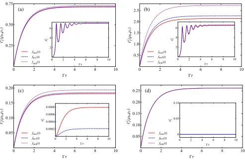
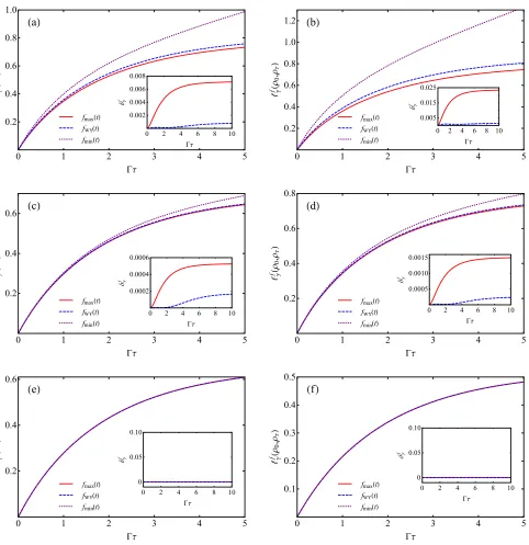
is equal to zero forθ₀¼π=2andω₀¼0(β¼0). Thus, the speed of evolution gf is described solely by the term F given in Eq.(38)and arising only from the populations of the evolved state. In this case, the speed of evolution remains invariant for any contractive Riemannian metric since F is common to all of them. However, it is still susceptible to changes depending on the purity and time. Let us now investigate how the QSLs in Eq.(17)behave by considering the quantum Fisher information metric and the Wigner-Yanase information metric, whose geodesic lengths are known analytically. In the insets of Fig.3, we compare the tightness parameterδfγ, as defined in Eq.(19),

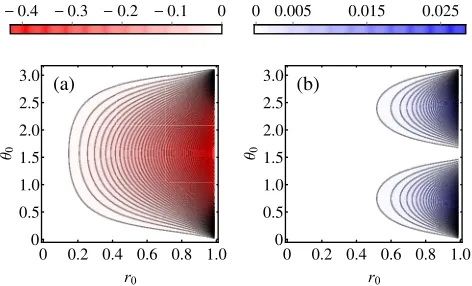
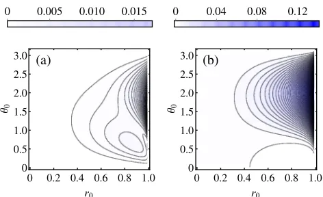
when considering these two metrics, for a parallel dephas-ing dynamical evolution. We can see that for β¼8, the dynamics does not saturate the bound for either of the two metrics, although the quantum Fisher information metric provides, in general, a slightly tighter QSL. On the other hand, whenβ¼0andθ₀¼π=2, we have that the QSL is saturated for both metrics, whereas for β¼0 and θ0¼π=4, it is instead the Wigner-Yanase information metric that provides us with a slightly tighter lower bound. More generally, it is sufficient to compare the difference between the tightness indicators δQFγ −δWIγ for the two metrics in the whole parameter space of the parallel dephasing model in order to identify in which regime each of the two corresponding bounds is the tightest. This analysis is reported in Fig. 4, showing that the Wigner-Yanase information metric does lead, in general, to a tighter QSL when the frequencyω₀is sufficiently small. This is in stark contrast to the case of unitary evolutions, discussed in the previous section, and constitutes a first demonstration of the usefulness of our generalized approach to speed limits in quantum dynamics.

max WY min

max WY min

max WY min

max WY min

FIG. 3. Evolution path lengthslfγ for parallel dephasing processes by considering the contractive Riemannian metrics corresponding to the following MC functions: fQFðtÞ ¼fmaxðtÞ (red solid line), fWYðtÞ (blue dashed line), and fminðtÞ (purple dotted line) for

Transversal dephasing.—We now focus on the case of transversal dephasing noise, which lets an initial state ρ0 evolve as ρt¼ ð1=2Þ

P₃

i;j¼0Sijσiρσj, where S is a 4×4

Hermitian matrix whose nonvanishing elements are given by S₀₀¼aþb, S₁₁¼dþf, S₂₂¼d−f, S₃₃ ¼a−b,

S₀₃¼ic, andS₃₀¼−ic, with

a¼1

2ð1þe−uÞ; ð40Þ

b¼e−u=2_{coshðΩu=2Þ; ð41Þ}

c¼2βe −u=2

Ω sinhðΩu=2Þ; ð42Þ

d¼1

2ð1−e−uÞ; ð43Þ

f¼e −u=2

Ω sinhðΩu=2Þ; ð44Þ

whereu¼Γt,Ω¼pffiffiffiffiffiffiffiffiffiffiffiffiffiffiffi1−4β2 andβ¼ω0=Γ. It is worth-while noticing that the transversal dephasing channel is also unital; i.e., it leaves the maximally mixed state invariant. This channel has proven to be of fundamental interest within the burgeoning field of noisy quantum metrology, as shown in Chaveset al.[59,60]. More precisely, transversal dephasing noise stands as the relevant scenario whereby one can attain a precision in the estimation of the parameter ω0that scales superclassically with the number of qubits, even if such noise applies independently to each qubit (while any superclassical advantage is lost in the case of parallel dephasing noise).

By writing the spectral decomposition of the density operatorρt, we get

ρt¼

X

j¼

pjjθt;ϕtijhθt;ϕtjj; ð45Þ

wherep¼ ð1=2Þð1þr0ξ~tÞ and

jθt;ϕti ¼ 1

N½½ð2a−1Þcosθ0 ~ ξtj0i

þ ½ðbþicÞeiϕ0þ_fe−iϕ0_sinθ

0j1i; ð46Þ

with

~ ξt¼

ffiffiffiffiffiffiffiffiffiffiffiffiffiffiffiffiffiffiffiffiffiffiffiffiffiffiffiffiffiffiffiffiffiffiffiffiffiffiffiffiffiffiffiffiffiffiffiffiffiffiffiffiffi ð2a−1Þ2cos2θ₀þζ~tsin2θ0

q

; ð47Þ

~

ζt¼b2þc2þf2þ2f½bcosð2ϕ0Þ−csinð2ϕ0Þ; ð48Þ

and N a normalization constant. By putting the above equations into Eqs.(15)and(16), one obtains expressions that are too cumbersome to be reported here. However, when restricting to the relevant case of an initial plus state (which is an optimal probe state for frequency estimation), i.e.,ρ₀¼ jþihþj withjþi ¼ ðj0i þ j1iÞ=pffiffiffi2, one obtains the following simple expressions:

F ¼ β4 Ω4

e−u_sinh2_ðΩu=2Þ

ð1−e−uGÞG ; ð49Þ

Qf_¼ β2

8Ge−ucfðpþ; p−Þ; ð50Þ

where

G¼ 1

Ω2½coshðΩuÞ þΩsinhðΩuÞ−4β2: ð51Þ

Let us now analyze the behavior of the QSLs in Eq.(17) corresponding to the quantum Fisher information metric and the Wigner-Yanase information metric when consid-ering the transversal dephasing dynamics. In Fig.5, we can see that, initializing such dynamics with a plus state, for small enough Γ and ω0, the Wigner-Yanase information provides a QSL that is tighter (in particular, at short times) than the one corresponding to the quantum Fisher infor-mation. One might identify, more generally, the region of parameters in which this behavior occurs by studying the trade-off between the respective tightness indicatorsδfγ for an arbitrary initial state, as in the previous case, although such a study does not add any further insight and is not reported here.

Once more, the present analysis shows that our approach applies straightforwardly to obtain novel, tighter bounds in dynamical cases of interest for quantum technologies, as 0.4 0.3 0.2 0.1 0

(a)

0 0.2 0.4 0.6 0.8 1.0 0

0.5 1.0 1.5 2.0 2.5 3.0

0 0.005 0.015 0.025

(b)

0 0.2 0.4 0.6 0.8 1.0 0

0.5 1.0 1.5 2.0 2.5 3.0

FIG. 4. Contour plot of the difference Δδγ≡δQFγ −δWYγ

corroborated here, in particular, for the metrologically relevant case of transversal dephasing noise.

2. Amplitude damping channel

We now consider another canonical model of noise, namely, dissipation modeled by an amplitude damping channel acting on a single qubit. For the amplitude damp-ing channel, we have the followdamp-ing Kraus operators:

~

K₀¼

_{1 0}

0 ffiffiffiffiffiffiffiffiffiffiffiffi1−λt

p

; K~₁¼

₀ ffiffiffiffi

λt

p

0 0

; ð52Þ

with λt¼1−e−Γt, and 1=Γ is the characteristic time of

the process [61], satisfying only P_jK~†_jK~j¼I since this

channel is not unital. The effect of amplitude damping consists in shrinking the Bloch sphere towards the north pole, or the statej0i. In this case, it is easy to verify that the evolved state ρt¼

P

jK~jρ0K~†j¼ ð1=2ÞðIþ~rt·~σÞ has the

following spectral decomposition:

ρt¼

X

j¼

p_jjθ_t;ϕ_ti_jhθ_t;ϕ_tj_j; ð53Þ

where p ¼1₂ð1ϑtÞand

jθt;ϕti¼ 1ffiffiffiffiffiffiffi

N

p ½ðςtϑtÞj0i þeiϕ0r0

ffiffiffiffiffiffiffiffiffiffiffiffi

1−λt

p

sinθ₀j1i;

ð54Þ

with

ϑt¼

ffiffiffiffiffiffiffiffiffiffiffiffiffiffiffiffiffiffiffiffiffiffiffiffiffiffiffi

1−ζtð1−λtÞ

p

; ð55Þ

ζt¼1−r20þλtð1−r0cosθ0Þ2; ð56Þ

ςt¼λtþr0ð1−λtÞcosθ0; ð57Þ

and N a normalization constant. By putting the above equations into Eqs.(15)and(16)one obtains, respectively,

F ¼½ζt−ð1−λtÞð1−r0cosθ0Þ22

16ϑ2

tζtð1−λtÞ

ð58Þ

and

Qf_¼r20sin2θ0ð2−ςtÞ2cfðpþ; p−Þ

32ϑ2

tð1−λtÞ

: ð59Þ

As in the case of the parallel dephasing channel, neither contributionF orQf_{to the speed of evolutiong}f_depends

on the initial azimuthal angleϕ₀. However, contrarily to the parallel dephasing channel case, here the purely quantum contributionQf vanishes only for θ₀¼0;π, whereas the termF vanishes in neither of these cases nor forθ0¼π=2, as expected due to the fact that now only the north pole, and not the entirezaxis of the Bloch sphere, is left invariant by the dynamics.

In Fig. 6, we compare the evolution path lengths appearing in the right-hand side of Eq. (17) and corre-sponding to the usual contractive Riemannian metrics, i.e., the quantum Fisher information metric, the Wigner-Yanase information metric, and the metric corresponding to the minimal MC function, by again changing the initial purity

r₀and polar angleθ0. First, Figs.6(e)and6(f)exhibit the following behavior: fixing the initial polar angleθ₀¼0, the speed of evolution decreases as we increase the initial purityr₀. This feature highlights the fact that the north pole of the Bloch sphere is unaffected by the amplitude damping channel. Moreover, according to Eq. (59), the purely quantum contribution Qf _{vanishes identically for θ0¼0,}

and the speed of evolutiongand corresponding evolution path length in Eq.(17)become independent of the choice of the MC functionf. The nontrivial contribution to the speed of evolution is, in this case, exclusively due to the term F, which depends solely on the populations pj of

the evolved state.

Let us now analyze the behavior of the QSLs in Eq.(17)corresponding to the quantum Fisher information metric and the Wigner-Yanase information metric (see AppendixCfor details). In the insets of Fig.6, we compare the tightness indicators δfγ, as defined in Eq. (19), when considering these two metrics, for the amplitude damping channel. We can see that, in this case, the Wigner-Yanase information provides a QSL that is almost saturated (in particular, at short times), whereas the quantum Fisher 0 2 4 6 8 10

0.01 0.02 0.03

0 1 2 3 4 5 0.01

0.02 0.03 0.04

0 1 2 3 4 5 0.01

0.02 0.03 0.04

0 1 2 3 4 5 0.1

0.2 0.3 0.4 0.5

(a) (b)

(c) (d)

max WY

max WY

max WY max

WY

information does not, except in the case ofθ0¼0 where they both realize tight bounds. What is more, in Fig.7one can see that for almost all initial states, except for a small neighborhood of the north pole (which is the asymptotic state of the amplitude damping channel), δQF≥δWY and δWY≃0; i.e., the Wigner-Yanase information metric

provides us with a definitely tighter (and nearly saturated) QSL than the quantum Fisher information metric.

This reveals another important physical mechanism, distinct from dephasing, in which our generalized analysis leads to significantly tighter bounds than those established in previous literature, which, in this case, is clearly max

WY min

max WY min

max WY min

max WY min

max WY min

max WY min

demonstrated in almost all the parameter space of rel-evance. This highlights the power of our general approach to reach beyond the state of the art.

V. CONCLUSIONS

Based on the fundamental connection between the geometry of quantum states and their statistical distinguish-ability, we have exploited the fact that more than one privileged Riemannian metric appears in quantum mechan-ics in order to introduce a new infinite family of geometric quantum speed limits valid for any physical process, being it unitary or not. Specifically, each bona fide geometric measure of distinguishability gives rise to a different quantum speed limit which is particularly tailored to the case of initial mixed states and such that the contributions of the populations of the evolved state and of the coher-ences of its time variation are clearly separated. This work provides a comprehensive general framework that incor-porates previous approaches to quantum speed limits and leaves room for novel insights.

By investigating paradigmatic examples of unitary and noisy physical processes and of contractive Riemannian metrics, we have seen, in fact, how the choice of the quantum Fisher information, corresponding to an extremal metric and being ubiquitous in the existing literature, is only a special case, which does not always provide the tightest lower bound in the realistic case of open system dynamics. In particular, for parallel and transversal

dephasing, as well as amplitude damping dynamics, we defined a tighter quantum speed limit by means of another important but significantly less-studied Riemannian metric, namely, the Wigner-Yanase skew information. The bound is useful in practical scenarios of noisy quantum metrology, especially in the case of transversal dephasing[59,60].

Our unifying approach provides a concrete guidance to select the most informative metric in order to derive the tightest bound for some particular dynamics of interest. We have formulated the problem as an optimization of a tightness indicator over all the infinite family of contractive quantum Riemannian metrics. The metric giving rise to the tightest bound is identified as the one whose geodesic is most tailored to the evolution under consideration [see Eq. (20)]. While such a problem can only be solved in restricted form at present, due to the fact that the quantum Fisher information and the Wigner-Yanase skew informa-tion are the only two metrics admitting known geodesics, further progress will be achievable when useful advances on the information geometry for other relevant metrics are recorded in the future.

It is important to remark that the family of speed limits provided in this paper are within the class of MT-like bounds. Following Ref.[62], it may be possible to imple-ment some adjustimple-ments to the adopted unified geometric approach in order to provide a generalized geometric interpretation to ML-like speed limits as well. This will be explored in a further study.

Our work readily suggests exploring how the nonunique-ness of a contractive Riemannian metric in the quantum-state space also affects other scenarios of relevance in quantum information processing. In several of these sce-narios, where the quantum Fisher information was adopted and privileged, our approach could lead to a more general investigation based on information geometry. For example, when considering parameter estimation, one of the para-digmatic tasks of quantum metrology, the inverse of the quantum Fisher information metric sets a lower bound to the mean-square error of any unbiased estimator for the parameters through the quantum Cramér-Rao bound [49,63]. This work inspires the quest to provide more general bounds on the sensitivity of quantum states to evolutions encoding unknown parameters, based on the infinite hierarchy of quantum Riemannian contractive geometries. It is useful to recall here that the Fisher information-based quantum Cramér-Rao bound for single-parameter estimation can only be achieved asymptotically in the limit of a large number of probes, and upon performing an optimal measurement given by projection into the eigenbasis of the symmetric logarithmic derivative, which is typically hard to implement in the experimental practice [63]. In the realistic case of a finite number of probes, corrections to the bound provide tighter estimates for the attainable estimation precision; these corrections were first investigated in Ref. [64] for the case of the 5

1 0 . 0 5

0 0 .

0 0.010 0

0 0.2 0.4 0.6 0.8 1.0 0

0.5 1.0 1.5 2.0 2.5 3.0

0 0.04 0.08 0.12

0 0.2 0.4 0.6 0.8 1.0 0

0.5 1.0 1.5 2.0 2.5 3.0

(a) (b)

FIG. 7. Contour plot of (a) the tightness indicator δWY γ of the

bound specified by the Wigner-Yanase information metric and (b) the differenceΔδγ≡δQFγ −δWYγ between the tightness

param-eter corresponding to the quantum Fisher information metric and the one corresponding to the Wigner-Yanase information metric, for the amplitude damping process as a function ofr₀andθ₀, for Γτ¼10. The QSL constructed with the Wigner-Yanase skew information is nearly globally optimal (asδWY

γ ≃0) and tighter

quantum Fisher information. Motivated by more recent works by Brody[65]and Brody and Graefe[66], in which the Wigner-Yanase skew information has been interpreted rather naturally as the speed of mixed quantum-state evolution, and by the analysis of the present work (which includes metrologically relevant settings such as frequency estimation under transversal dephasing[59,60]), we believe it is worth investigating finite-size corrections to the Cramér-Rao inequality based on the Wigner-Yanase infor-mation, in order to determine how tight the bound can be for practical purposes, in particular, for the estimation of parameters encoded in open system dynamics.

Furthermore, within the burgeoning field of quantum thermodynamics, our approach could provide an infinite class of generalizations of the classical thermodynamical length [67], originally based on the unique classical con-tractive Riemannian metric, to the quantum setting. Again, in the context of quantum thermodynamics, because of the close connections between geometry and entropy, it might be interesting to investigate the role played by the non-uniqueness of a contractive Riemannian geometry on the quantum-state space in the existence of many second laws of thermodynamics[68]. In the study of quantum criticality, within the condensed-matter realm, a geometric approach based on the fidelity, i.e., on the quantum Fisher information metric, proved to be fruitful [69]. Along the lines of this work, one could apply more general tools associated with any quantum Riemannian contractive metric, in order to seek further insights and sharper identification of quantum critical phenomena.

Finally, the general approach presented in this paper to pinpoint the tightest speed limits in quantum evolutions is readily useful for applications to quantum engineering and quantum control. Specifically, the present study allows one to certify that, in a particular implementation, quantum states have been driven at the ultimate speed limit[42]and their evolution cannot be sped up further: This occurs whenever saturation of one of our bounds is demonstrated. As our various examples show, this is not possible to verify only by considering the standard bound based on quantum Fisher information. For single-qubit evolutions, we showed that the latter is in fact the tightest for the idealized case of unitary dynamics, while our novel bound based on the Wigner-Yanase skew information can instead be significantly tighter in the most common instances of open dynamics, effectively yielding the optimal bound (even among all the other unverifiable Riemannian metrics) for amplitude damping dynamics, as certified by a nearly vanishing tightness indicator in such a case. Given that the Wigner-Yanase skew information is experimentally accessible [70], one can readily apply our results to current and future demonstrations to benchmark optimality of controlled quantum dynamics in the presence of such ubiquitous noise mechanisms.

In this respect, we would like to point out that an experimental investigation of the main results presented

here, for both closed and open system dynamics, can be achieved, in particular, using a highly controllable nuclear magnetic resonance setup, with no need for a complete quantum state tomography. In fact, dephasing and amplitude damping are naturally occurring sources of decoherence in such an implementation, and our results can be accessed by means of spin ensemble measurements, which constitute the conventional types of detection in such a technique[71,72]. An experimental investigation as described deserves a study on its own and will be reported elsewhere.

ACKNOWLEDGMENTS

We thank Dorje C. Brody, Tyler J. Volkoff, Frederico Brito, J. Carlos Egues, Paolo Gibilisco, and Fumio Hiai for fruitful discussions. The authors would like to acknowl-edge financial support from the Brazilian funding agencies CNPq (Grants No. 445516/2014-3, No. 401230/2014-7, No. 305086/2013-8, No. 304955/2013-2, and No. 443828/ 2014-8), CAPES (Grant No. 108/2012), the Brazilian National Institute of Science and Technology of Quantum Information (INCT/IQ), and the European Research Council (ERC StG GQCOP, Grant No. 637352).

D. P. P. and M. C. contributed equally to this work.

APPENDIX A: UNITARY DYNAMICS

In this appendix, we prove that the geometric QSL corresponding to the quantum Fisher information metric is tighter than the one corresponding to the Wigner-Yanase information metric, when considering any single-qubit unitary dynamics.

Let us consider a one-qubit stateρ₀¼ ð1=2ÞðIþ~r₀·~σÞ,

where~r₀¼ fr₀sinθ₀cosϕ₀; r₀sinθ₀sinϕ₀; r₀cosθ₀gand

~

σ is the vector of Pauli matrices, which undergoes the generic unitary evolutionγ specified byρ_t¼U_tρ₀U†_t. We want to prove that for anyρ₀ andUt, the following holds

(we drop the subscriptγin the remainder of this section for simplicity),

δQF_≤δWY_{; ðA1Þ}

where δf _{is the tightness indicator corresponding to the}

contractive Riemannian metricgf _{with MC functionf, as}

defined in Eq.(19). In order to prove the above inequality, we just need to prove that

lQF_ðρ

0;ρτÞ

lWY_ðρ

0;ρτÞ≤

LQF_ðρ

0;ρτÞ

LWY_ðρ

0;ρτÞ

; ðA2Þ

where we denote bylf_ðρ

We know that

lf_{ðρ0;ρτÞ ¼}

Z _τ

0

ffiffiffiffiffi gf

q

dt; ðA3Þ

where gf¼FþQf and

F ¼1 4

X2

j¼1

1

pj

dpj

dt ₂

; ðA4Þ

Qf_¼1

2cfðp1; p2Þðp1−p2Þ2A12A21; ðA5Þ

withpjbeing the eigenvalues of the evolved stateρt,Ajl¼

ihjjðd=dtÞjli being quantities that depend on the eigen-states jjiof the evolved stateρt, and finally

cQFðp₁; p₂Þ ¼ 2

p₁þp₂¼2; ðA6Þ

cWY_ðp

1; p2Þ ¼_ð ffiffiffiffiffi_p 4 1 p _þ ffiffiffiffiffi

p₂

p _Þ2: ðA7Þ

Since the eigenvalues p₁;2¼ ð1r0Þ=2 of the unitarily

evolving one-qubit state are time independent, it immedi-ately follows that

F ¼0; ðA8Þ

cWY_ðp

1; p2Þ ¼ 4

1þpffiffiffiffiffiffiffiffiffiffiffiffi1−r2₀; ðA9Þ

so that

lQF_ðρ

0;ρτÞ

lWY_ðρ

0;ρτÞ¼

ffiffiffiffiffiffiffiffiffiffiffiffiffiffiffiffiffiffiffiffiffiffiffiffi cQFðp₁; p₂Þ cWY_ðp

1; p2Þ

s

¼

ffiffiffiffiffiffiffiffiffiffiffiffiffiffiffiffiffiffiffiffiffiffiffiffiffi

1þpffiffiffiffiffiffiffiffiffiffiffiffi1−r2₀

2

s

:

ðA10Þ

On the other hand, because of Eqs. (5)and(6), we have

LQF_ðρ

0;ρτÞ

LWY_ðρ

0;ρτÞ¼

arccos½pffiffiffiffiffiffiffiffiffiffiffiffiffiffiffiffiffiffiFðρ₀;ρ_τÞ

arccos½Aðρ₀;ρ_τÞ ; ðA11Þ

where the analytical formulas of the fidelityFðρ₀;ρ_τÞand the affinityAðρ0;ρτÞfor any pair of one-qubit statesρ0and ρτ are the following[29,73,74]:

Fðρ₀;ρ_τÞ ¼1

2

1þ~r₀·~r_τ þ

ffiffiffiffiffiffiffiffiffiffiffiffiffiffiffiffiffiffiffiffiffiffiffiffiffiffiffiffiffiffiffiffiffiffiffiffiffiffiffiffi ð1−j~r₀j2Þð1−j~r_τj2Þ

q

;

ðA12Þ

Aðρ₀;ρ_τÞ ¼1

4

ϵþ

0ϵþτ þϵ−0ϵ−τ _j~r_~r0·~rτ 0jj~rτj

; ðA13Þ

with

ϵ

a ¼

ffiffiffiffiffiffiffiffiffiffiffiffiffiffiffi

1þ j~r_aj q

ffiffiffiffiffiffiffiffiffiffiffiffiffiffiffi1−j~r_aj q

; ðA14Þ

anda¼0;τ.

Sinceρτ ¼Uτρ0U†τ, we get

j~r₀j ¼ j~r_τj ¼r₀; ðA15Þ

~r₀·~r_τ¼ j~r₀jj~r_τjcosðφ_0;τÞ ¼r2₀cosðφ_0;τÞ; ðA16Þ

withφ0;τbeing the angle between the vectors~r0and~rτ, so

we simply get

LQF_ðρ

0;ρτÞ

LWY_ðρ

0;ρτÞ

¼ arccos

ffiffiffiffiffiffiffiffiffiffiffiffiffiffiffiffiffiffiffiffiffiffiffiffiffiffiffiffiffiffiffiffiffiffiffiffiffiffiffiffiffiffiffiffiffiffi

1

2ð2−r20þr20cosðφ0;τÞÞ

q

arccosf1₂½cosðφ0;τÞð1−

ffiffiffiffiffiffiffiffiffiffiffiffi

1−r2₀ p

Þ þ1þpffiffiffiffiffiffiffiffiffiffiffiffi1−r2₀g:

ðA17Þ

Overall, by collecting Eqs.(A10)and(A17), we need to prove that

ffiffiffiffiffiffiffiffiffiffiffiffiffiffiffiffiffiffiffiffiffiffiffiffiffi

1þpffiffiffiffiffiffiffiffiffiffiffiffi1−r2₀

2

s

≤ arccos

ffiffiffiffiffiffiffiffiffiffiffiffiffiffiffiffiffiffiffiffiffiffiffiffiffiffiffiffiffiffiffiffiffiffiffiffiffiffiffiffiffiffiffiffiffiffi

1

2ð2−r20þr20cosðφ0;τÞÞ

q

arccosf1₂½cosðφ₀;τÞð1−

ffiffiffiffiffiffiffiffiffiffiffiffi

1−r2₀ p

Þ þ1þpffiffiffiffiffiffiffiffiffiffiffiffi1−r2₀g:

ðA18Þ

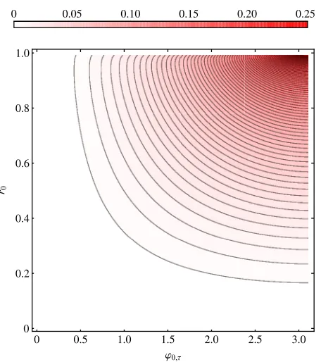
The difference between the right-hand side and left-hand side of the above inequality is represented in Fig. 8as a function ofr₀∈½0;1½andφ0;τ ∈½0;π. As it can be easily

seen, this difference is always non-negative, i.e., the inequality (A2) is always satisfied. In particular, this difference is zero when either r₀¼0or ~r₀·~r_τ ¼r2₀, i.e., whenφ_0;τ ¼0, as can be proved by checking that

lim

~r0·~rτ→r2₀

arccos

ffiffiffiffiffiffiffiffiffiffiffiffiffiffiffiffiffiffiffiffiffiffiffiffiffiffiffiffiffiffiffiffiffiffiffi

1

2ð2−r20þ~r0·~rτÞ

q

arccosf1₂½~r0·~rτ r2₀ ð1−

ffiffiffiffiffiffiffiffiffiffiffiffi

1−r2₀ p

Þ þ1þpffiffiffiffiffiffiffiffiffiffiffiffi1−r2₀g

¼

ffiffiffiffiffiffiffiffiffiffiffiffiffiffiffiffiffiffiffiffiffiffiffiffiffi

1þpffiffiffiffiffiffiffiffiffiffiffiffi1−r2₀

2

s

: ðA19Þ

lf_ðρ

0;ρτÞ

lh_ðρ

0;ρτÞ¼

ffiffiffiffiffiffiffiffiffiffiffiffiffiffiffiffiffiffiffiffiffi cfðp₁; p₂Þ ch_ðp

1; p2Þ

s

: ðA20Þ

However, we also note that this is only true in the one-qubit unitary case. If the dimensionality of the system is higher than 2, thenQf_{becomes a nontrivial sum, as defined}

in Eq. (16), so that the various time-independent coeffi-cientscfðpj; plÞcannot be extracted from the path integral

as we have just done above. On the other hand, Eq.(A17) seems hard to generalize to other contractive Riemannian metrics since the analytical expressions of the correspond-ing geodesic lengths are still unknown. We can thus leave the following conjecture: For any one-qubit unitary dynamics, the quantum Fisher information is the metric which provides the tightest QSL among all contractive Riemannian metrics on the quantum-state space; i.e., it is the metric solving the optimization problem in Eq. (20). Here, we have shown that the conjecture holds when the optimization is restricted to the quantum Fisher information and the Wigner-Yanase skew information metrics only.

APPENDIX B: PARALLEL AND TRANSVERSAL DEPHASING

In this appendix, we show how to compute all the quantities playing a role in Eq. (17), for the parallel and transversal dephasing dynamics, when considering the quantum Fisher information metric, the Wigner-Yanase

information metric, and the metric corresponding to the minimal MC function.

Let us start from the case of parallel dephasing and from the quantum Fisher information metric. Recall that its MC function is the maximal one, i.e., f_QFðtÞ ¼f_maxðtÞ ¼

ð1þtÞ=2, implying that cf_{ðx; yÞ ¼2=ðxþyÞ and, since}

TrðρtÞ ¼pþþp−¼1, cfðpþ; p−Þ ¼2. It is possible to

provide an analytical expression for the path length corresponding to such a MC function as follows:

lQF

γ ðρ0;ρτÞ ¼1

2

ffiffiffiffiffiffiffiffiffiffiffiffiffiffiffiffiffiffiffiffiffiffiffiffiffiffiffi ð1þβ2_ÞhΔZˆ_i

q

½Eðarcsinα;κ2Þ

−Eðarcsinðαe−ΓτÞ;κ2Þ; ðB1Þ

whereEðy;κ2Þ ¼R₀ydy0pffiffiffiffiffiffiffiffiffiffiffiffiffiffiffiffiffiffiffiffiffiffiffi1−κ2sin2y0 is the elliptic inte-gral of the second kind,β¼ω0=Γ,κ2¼β2=ð1þβ2Þ, and

hΔZˆi ¼1−r2₀cos2θ₀; α¼

ffiffiffiffiffiffiffiffiffiffiffiffiffiffiffiffiffiffiffiffi

1−1−r20 hΔZˆi s

; ðB2Þ

with hΔZˆi ¼Trðρtσz2Þ−TrðρtσzÞ2 being the variance of

the Pauli matrixσ_z. Specifically, when considering the case in whichω₀¼0, i.e.,β¼0andκ¼0, the path length in Eq.(B1)becomes

lQF

γ ðρ0;ρτÞ ¼1

2

ffiffiffiffiffiffiffiffiffiffiffi hΔZˆi q

½arcsinα−arcsinðαe−ΓτÞ: ðB3Þ

Furthermore, the geodesic length corresponding to such a metric can be readily obtained by using Eqs. (5) and(A12), with

j~r_τj ¼r0ξτ;

~r₀·~r_τ ¼r2₀½cos2θ₀þq_τsin2θ₀cosðω₀τÞ: ðB4Þ

Now considering the Wigner-Yanase information metric, we know that the corresponding MC function isfWYðtÞ ¼

ð1=4Þðpffiffitþ1Þ2 so that cfðpþ; p−Þ ¼4=ðppffiffiffiffiffiffiþþpffiffiffiffiffiffip−Þ2.

Hence, the path length corresponding to the Wigner-Yanase information metric is given by

lWY

γ ðρ0;ρτÞ ¼1₂

ffiffiffiffiffiffiffiffiffiffiffiffiffiffiffiffiffiffiffiffiffiffiffiffiffiffi ð1þβ2_ÞhΔZˆi

q Z _Γτ

0 duαe

−u_Ψ

uðr0;θ0;κÞ;

ðB5Þ

where

Ψuðr0;θ0;κÞ ¼

ffiffiffiffiffiffiffiffiffiffiffiffiffiffiffiffiffiffiffiffiffiffiffiffiffiffiffiffiffiffiffiffiffiffiffiffiffiffiffiffiffiffiffiffiffiffiffiffiffiffiffiffiffiffiffi Ωuðr0;θ0;κÞ þ

1−κ2_α2_e−2u

1−α2_e−2u

s

ðB6Þ

and 0 0.05 0.10 0.15 0.20 0.25

0 0.5 1.0 1.5 2.0 2.5 3.0 0

0.2 0.4 0.6 0.8 1.0